Chapter 30 Likelihood based inference
Motivating scenario: We want to make inferences on data from any type of null model.
30.1 Likelihood Based Inference
We have focused extensively on the normal distribution in our linear modeling. This makes sense, many things are approximately normally, but definitely not everything. We have also assumed independence – this is a more dicey because we usually only have independence in really carefully done experiments – but whatever.
The good news is that we can break free from the assumptions of linear models and build and make inference under any model we can appropriately describe by an equation under likelihood-based inference! We can even model things like phylogenies or genome sequences or whatever.
30.1.1 Remember probabilities?
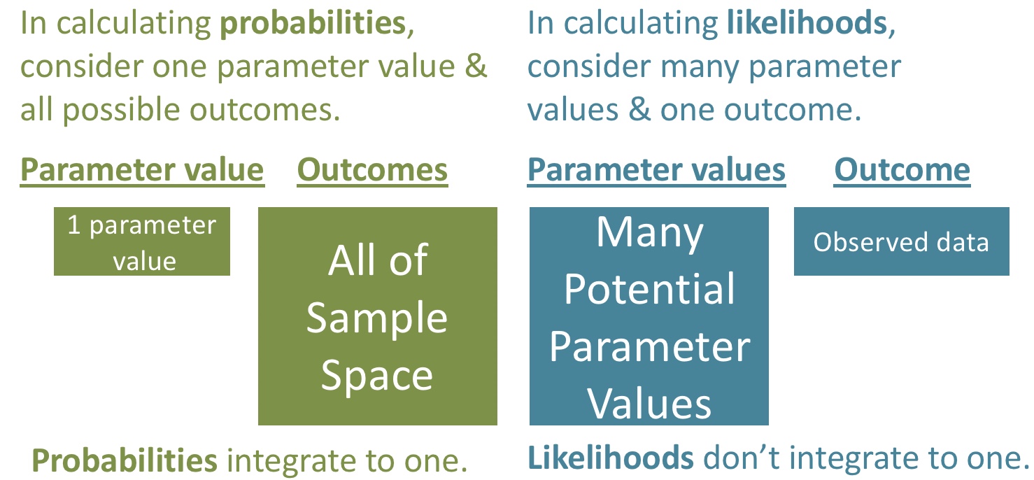
Remember, a probability is the proportion of times a model would produce the result we are considering. When we think about probabilities, we think about one model, and consider all the potential outcome. For a given model, all the probabilities (or probability densities) will sum (or integrate) to one.
30.1.2 Likelihoods
The mathematical calculation for a likelihood is the EXACT SAME as the calculation of a probability.
The big difference is our orientation — in a likelihood, we think of the outcome as fixed, and consider the different models that could have generated this outcome. So we think of a likelihood as a conditional probability.
\[P(Data | Model) = \mathscr{L}(Model | Data)\]
30.1.3 Log liklihoods
If data are independent, we can calculate the likelihood of all of our data by taking the product of each individual likelihood. This is great, but inroduces some challenges
- Multiplying a lot of probabilities can make a really small probability. In fact these numbers can get so small that computers lose track of them.
- They are not great for math.
So we take the log of each likelihood and sum them all, because adding in log space is like multiplying in linear space – e.g. 0.5 * 0.2 = 0.1. and log(0.5) + log(0.2) = -2.302585 and \(e^{-2.302585} = 0.1\).
So we almost always deal with log likelihoods instead of likelihoods.
30.2 Log Likelihood of \(\mu\)
How can we calculate likelihoods for a parameter of a normal distribution? Here’s how!
Say we had a sample with values 0.01, 0.07, and 2.2, and we knew the population standard deviation equaled one, but we didn’t know the population mean. We could find the likelihood of a proposed mean by multiplying the probability of each observation, given the proposed mean. So the likelihood of \(\mu = 0 | \sigma = 1, \text{ and } Data = \{0.01, 0.07, 2.2\}\) is
dnorm(x = 0.01, mean = 0, sd = 1) * dnorm(x = 0.07, mean = 0, sd = 1) * dnorm(x = 2.20, mean = 0, sd = 1)## [1] 0.005632A more compact way to write this is dnorm(x = c(0.01, 0.07, 2.20), mean = 0, sd = 1) %>% prod(). Remember we multiply because all observations are independent.
For both mathematical and logistical (computers have trouble with very small numbers) reasons, it is usually better to work wit log likelihoods than linear likelihoods. Because multiplying on linear scale is like adding on log scale, the log likelihood for this case is dnorm(x = c(0.01, 0.07, 2.20), mean = 0, sd = 1, log = TRUE) %>% sum() = -5.1793. Reassuringly, log(0.00563186) = -5.1793.
30.2.1 The likelihood profile
We can consider a bunch of other plausible parameter values and calculate the (log) likelihood of the data for all of these “models”. This is called a likelihood profile. We can find a likelihood profile as
obs            <- c(0.01, 0.07, 2.2)
proposed.means <- seq(-1, 2, .001)
tibble(proposed_means = rep(proposed.means , each = length(obs)),
       observations   = rep(obs, times = length(proposed.means)),
       log_liks       = dnorm(x = observations, mean = proposed_means, sd = 1, log = TRUE)) %>%
  group_by(proposed_means) %>%
  summarise(logLik = sum(log_liks)) %>%
  ggplot(aes(x = proposed_means, y = logLik))+
  geom_line()
30.2.2 Maximum likelihood estimate
How can we use this for inference? Well, one estimate of our parameter is to the one that “maximizes the likelihood” of our data (e.g. the x value corresponding to the largest value in the figure above).
Note that this is NOT the parameter value with the best chance of being right (that’s a Bayesian question), but rather this is the parameter that, if true, would have the greatest chance of generating our data.
Drake helped me clarify something pic.twitter.com/S2nK6bpHSv
— Doc Edge (@DocEdge85) March 29, 2021
We can find the maximum likelihood estimate as
tibble(proposed_means = rep(proposed.means , each = length(obs)),
       observations   = rep(obs, times = length(proposed.means)),
       log_liks       = dnorm(x = observations, mean = proposed_means, sd = 1, log = TRUE)) %>%
  group_by(proposed_means) %>%
  summarise(logLik = sum(log_liks)) %>%
  filter(logLik == max(logLik)) %>%
  pull(proposed_means)
## [1] 0.76Which equals the mean of our observations mean(c(0.01, 0.07, 2.2)) = 0.76. More broadly, for normally distributed data, the maximum likelihood estimate of a population mean is the sample mean.
30.3 Likelihood based inference: Uncertainty and hypothesis testing.
We calculate the likelihoods and do likelihood-based inference for samples from a normal the exact same way as we did previously.
Because this all relies on pretending we are using population parameters. So we calculate the sd as the distance of each data point from the proposed mean, and divide by n rather than n-1.
30.3.1 Example 1: Are species moving uphill
Remember in Chapter 18, we looked at data from, Chen et al. (2011) who tested the idea that organisms move to higher elevation as the climate warms. To test this, they collected data from 31 species, plotted below (Fig 30.1).
range_shift_file <- "https://whitlockschluter3e.zoology.ubc.ca/Data/chapter11/chap11q01RangeShiftsWithClimateChange.csv"
range_shift <- read_csv(range_shift_file) %>%
  mutate(x = "", uphill = elevationalRangeShift > 0)

ggplot(range_shift, aes(x = x, y = elevationalRangeShift))+
  geom_jitter(aes(color = uphill), width = .05, height = 0, size = 2, alpha = .7)+
  geom_hline(yintercept = 0, lty= 2)+
  stat_summary(fun.data = "mean_cl_normal") +
  theme(axis.title.x = element_blank())
FIGURE 30.1: Change in the elevation of 31 species. Data from Chen et al. (2011).
We then conducted a one sample t-test against of the null hypothesis that there has been zero net change on average.
lm(elevationalRangeShift ~ 1, data = range_shift) %>%
  summary()
##
## Call:
## lm(formula = elevationalRangeShift ~ 1, data = range_shift)
##
## Residuals:
## Min 1Q Median 3Q Max
## -58.63 -23.38 -3.53 24.12 69.27
##
## Coefficients:
## Estimate Std. Error t value Pr(>|t|)
## (Intercept) 39.33 5.51 7.14 6.1e-08 ***
## ---
## Signif. codes:
## 0 '***' 0.001 '**' 0.01 '*' 0.05 '.' 0.1 ' ' 1
##
## Residual standard error: 30.7 on 30 degrees of freedom30.3.1.1 Calculate log likelihoods for each model
First we grab our observations, write down our proposed means – lets say from negative one hundred to two hundred in increments of .01.
observations   <-  pull(range_shift, elevationalRangeShift)
proposed_means <- seq(-100,200,.01)- Copy our data as many times as we have parameter guesses
- Calculate the population variance for each proposed parameter value,
- Calculate for each guess log likelihood of each observation at each proposed parameter value
lnLik_uphill_calc <- tibble(obs = rep(observations, each = length(proposed_means)), # Copy observations a bunch of times
                        mu  = rep(proposed_means, times = length(observations)),# Copy parameter guesses a bunch of times
                        sqr_dev = (obs - mu)^2 )%>%
  group_by(mu) %>%
  mutate(var = sum((obs - mu)^2 ) / n(), #  Calculate the population variance for each proposed parameter value
         lnLik = dnorm(x = obs, mean = mu, sd = sqrt(var), log = TRUE)) #Calculate for each guess log likelihood of each observation at each proposed parameter value
FIGURE 30.2: log likelihoods of each data point for 100 proposed means (a subst of those investigated above)
Find the likelihood of each proposed mean by adding in log scale (i.e. multiplying in linear scale because these are all independent) the probability of each observation given the proposed parameter value.
lnLik_uphill <- lnLik_uphill_calc %>%
  summarise(lnLik = sum(lnLik))

ggplot(lnLik_uphill, aes(x = mu, y = lnLik))+
  geom_line()
FIGURE 30.3: likelihood profile for proposed mean elevational shift in species examined by data from Chen et al. (2011)
30.3.1.2 Maximium likelihood / Confidence intervals / Hypothesis testing
We can use the likelihood profile (Fig 30.3) to do standard things, like
- Make a good guess of the parameter,
- Find confidence intervals around this guess,
- Test null hypotheses that this guess differs from the value proposed under the null
First lets find our guess – called the maximum likelihood estimator (MLE)
MLE <- lnLik_uphill %>%
  filter(lnLik == max(lnLik))                                                                                                                ; data.frame(MLE)
## mu lnLik
## 1 39.33 -149.6Reassuringly, this MLE matches the simple calculation of the mean mean(observations) = 39.33.
NOTE The model from the lm() function will be the MLE. So we can use this to caucalte it’s likelihood.
Either “by hand” from the model’s output
lm(elevationalRangeShift ~ 1, data = range_shift) %>%
    augment() %>%
    mutate(sd = sqrt(sum(.resid^2) / n()),
           logLiks = dnorm(x = .resid, mean = 0 , sd = sd, log = TRUE)) %>%
    summarise(log_lik = sum(logLiks))                                                                                                   %>% data.frame()
## log_lik
## 1 -149.6Or with the logLik() function.
lm(elevationalRangeShift ~ 1, data = range_shift) %>%
  logLik()
## 'log Lik.' -149.6 (df=2)Uncertainty
We need one more trick to use the likelihood profile to estimate uncertainty
log likelihoods are roughly \(\chi^2\) distributed with degrees of freedom equal to the number of parameters we’re inferring (here, just one – corresponding to the mean). So for 95% confidence intervals are everything within qchisq(p = .95, df =1) /2 = 1.92 log likelihood units of the MLE
CI <- lnLik_uphill %>%
  mutate(dist_from_MLE =  max(lnLik) - lnLik) %>%
  filter(dist_from_MLE < qchisq(p = .95, df =1) /2) %>%
  summarise(lower_95CI = min(mu),
            upper_95CI = max(mu))                                                                                               ; data.frame(CI)
## lower_95CI upper_95CI
## 1 28.38 50.28Hypothesis testing by the likelihood ratio test
We can find a p-value and test the null hypothesis by comparing the likelihood of our MLE (\(log\mathscr{L}(MLE|D)\)) to the likelihood of the null model (\(log\mathscr{L}(H_0|D)\)). We call this a likelihood ratio test, because we divide the likelihood of the MLE by the likelihood of the null – but we’re doing this in logs, so we subtract rather than divide.
\(log\mathscr{L}(MLE|D)\) = Sum the log-likelihood of each observation under the MLE =
pull(MLE, lnLik)= -149.594.\(log\mathscr{L}(H_0|D)\) = Sum the log-likelihood of each observation under the null =
lnLik_uphill%>% filter(mu == 0 ) %>% pull(lnLik)= -164.989.
We then calculate \(D\) which is simply two times this difference in lof likelihoods, and calcualte a p-value with it by noting that \(D\) is \(\chi^2\) distributed with degrees of freedom equal to the number of parameters we’re inferring (here, just one – corresponding to the mean).
D      <- 2 *  (pull(MLE, lnLik) -   lnLik_uphill%>% filter(mu == 0 ) %>% pull(lnLik)  )
p_val  <- pchisq(q = D, df = 1, lower.tail = FALSE)
c(D = D, p_val = p_val)
## D p_val
## 3.079e+01 2.875e-0830.4 Bayesian inference
We often can are about how probable our model is given the data, not the opposite. We can use likelihoods to solve this!!! Remember Bayes’ theorem: \((Model|Data) = \frac{P(Data|Model) \times P(Model)}{P(Data)}\). Taking this apart
- \((Model|Data)\) is called the posterior probability – the probability of our model after we know the data.
- \(P(Data|Model) = \mathscr{L}(Model|Data)\). This is the likelihood we just calculated.
- \(P(Model)\) is called the prior probability. This is the probability our model is true before we have data. We almost never know this, so we make something up that sounds reasonable…
- \(P(Data)\). The probability of our data, called the evidence. We find this through the law of total probability.
Today, we’ll arbitrarily pick a prior probability. This is a bad thing to do – out Bayesian inferences are only meaningful to the extent that a meaningfully interpret the posterior, and this relies on a reasonable prior. But we’re doing it as an example: – say our prior is that this is normally distributed around 0 with a standard deviation of 30.
bayes_uphill <- lnLik_uphill %>%
  mutate(lik   = exp(lnLik),
         prior = dnorm(x = mu, mean = 0, sd = 30) / sum(dnorm(x = mu, mean = 0, sd = 30) ),
         evidence  = sum(lik * prior),
posterior = (lik * prior) / evidence) 
We can grab interesting thing from the posterior distribution.
- For example we can find the maximum a posteriori (MAP) estimate as
bayes_uphill %>%
  filter(posterior == max(posterior))                                                                                                  %>% data.frame()
## mu lnLik lik prior evidence posterior
## 1 38.08 -149.6 1.049e-65 5.944e-05 8.55e-67 0.0007292Note that this MAP estimate does not equal our MLE as it is pulled away from it by our prior.
- We can grab the 95% credible interval. Unlike the 95% confidence intervals, the 95% credible interval has a 95% chance of containing the true parameter (if our prior is correct).
bayes_uphill %>%
  mutate(cumProb = cumsum(posterior)) %>%
  filter(cumProb > 0.025 & cumProb < 0.975)%>%
  summarise(lower_95cred = min(mu),
            upper_95cred = max(mu))                                                                                                %>% data.frame()
## lower_95cred upper_95cred
## 1 26.78 48.8830.4.1 Prior sensitivity
In a good world our priors are well calibrated.
In a better world, the evidence in the data is so strong, that our priors don’t matter.
A good thing to do is to compare our posterior distributions across different prior models. The plot below shows that if our prior is very tight, we have trouble moving the posterior away from it. Another way to say this, is that if your prior believe is strong, it would take loads of evidence to gr you to change it.

MCMC / STAN / brms
With more complex models, we usually can’t use the math above to solve Bayesian problems. Rather we use computer ticks – most notably the Markov Chain Monte Carlo MCMC to approximate the posterior distribution.
The programming here can be tedious so there are many programs – notable WINBUGS, JAGS and STAN – that make the computation easier. But even those can be a lot of work. Here I use the R package brms, which runs stan for us, to do an MCMC and do Bayesian stats. I suggest looking into this if you want to get stared, and learning STAN for more serious analyses
library(brms)
change.fit <- brm(elevationalRangeShift ~ 1,
    data   = range_shift,
    family = gaussian(),
    prior  = set_prior("normal(0, 30)",
                      class = "Intercept"),
    chains = 4,
    iter   = 5000)

change.fit$fit