Week 3 Data Structure (Part 2) & Control Flows

3.1 Matrix

In R, a matrix is a homogeneous 2d vector, that is, all the elements must be of the same type (e.g., numerical). Let’s create a 3 $\times$ 3 matrix that looks like:

\[\begin{pmatrix} 1 & 2 & 3\\ 4 & 5 & 6\\ 7 & 8 & 9 \end{pmatrix} \]

m1 <- matrix(c(1, 2, 3,
               4, 5, 6,
               7, 8, 9), 
             nrow = 3)
m1

##      [,1] [,2] [,3]
## [1,]    1    4    7
## [2,]    2    5    8
## [3,]    3    6    9

The created matrix above looks slightly different from what we wanted to create. In order to fill the elements of the matrix by rows, we need to add the argument byrow = T in the matrix() function.

m2 <- matrix(c(1,2,3,
               4,5,6,
               7,8,9), 
             nrow = 3, 
             byrow = T)

To figure out the total number of entries, use length().

length(m2)

## [1] 9

Now, let’s figure out the number of rows and the number of columns.

nrow(m2)

## [1] 3

ncol(m2)

## [1] 3

Addition and subtraction of matrices can be operated by + and -.

m1 + m2

##      [,1] [,2] [,3]
## [1,]    2    6   10
## [2,]    6   10   14
## [3,]   10   14   18

m1 - m2

##      [,1] [,2] [,3]
## [1,]    0    2    4
## [2,]   -2    0    2
## [3,]   -4   -2    0

If you write the general multiplication sign * between matrices and run, it will do element-wise multiplication. In other words, the scalars in the $i$th row and the $j$th column in each matrices will be multiplied to be the $i$th row and the $j$th column in the result matrix.

m1 * m2

##      [,1] [,2] [,3]
## [1,]    1    8   21
## [2,]    8   25   48
## [3,]   21   48   81

In the last chapter, we used brackets [] for subsetting a part of an atomic vector. Since a matrix is a 2-dimensional vector, we need to specify two numbers to refer to a specific scalar in a matrix. The first number represents a row and the second number represents a column. For example, running m1[1, 2] will return the scalar in the 1st row and the 2nd column in the matrix m1:

m1[1, 2]

## [1] 4

We can refer to a specific column or a specific row of the matrix by:

m1[, 3] # the third column of the matrix

## [1] 7 8 9

m1[2, ] # the second row of the matrix

## [1] 2 5 8

Of course, atomic vectors can be used inside the brackets to refer to a subset of a matrix.

m1[c(1, 3), 1:2]

##      [,1] [,2]
## [1,]    1    4
## [2,]    3    6

Row-wise/column-wise sums and means are obtained by:

rowSums(m1)

## [1] 12 15 18

rowMeans(m1)

## [1] 4 5 6

colSums(m1)

## [1]  6 15 24

colMeans(m1)

## [1] 2 5 8

You can add an atomic vector as a new row or a new column to a matrix.

rbind(m1, c(1, 2, 3))

##      [,1] [,2] [,3]
## [1,]    1    4    7
## [2,]    2    5    8
## [3,]    3    6    9
## [4,]    1    2    3

cbind(m1, c(1, 2, 3))

##      [,1] [,2] [,3] [,4]
## [1,]    1    4    7    1
## [2,]    2    5    8    2
## [3,]    3    6    9    3

rbind() and cbind() combine the matrix and the vector by rows or columns, respectively.

3.2 Data frame

Data frames are used as the fundamental data structure in R. Each row represents a case (e.g., students, customer), and each column represents a variable (e.g., test score, age, names, id). Data frames and matrices share a lot of properties. Data frames are 2-dimensional vectors. While all the elements in a matrix must be homogeneous, each column (atomic vector) in a data frame can be different types. For example, one column vector of a data frame can be the ages (numeric), another column vector of a data frame can be the names (character).

Let’s try to import and handle a data frame in R. Right click the following link and Save Link as... to save the example file. Please remember under which directory you saved the file. example2.1.txt

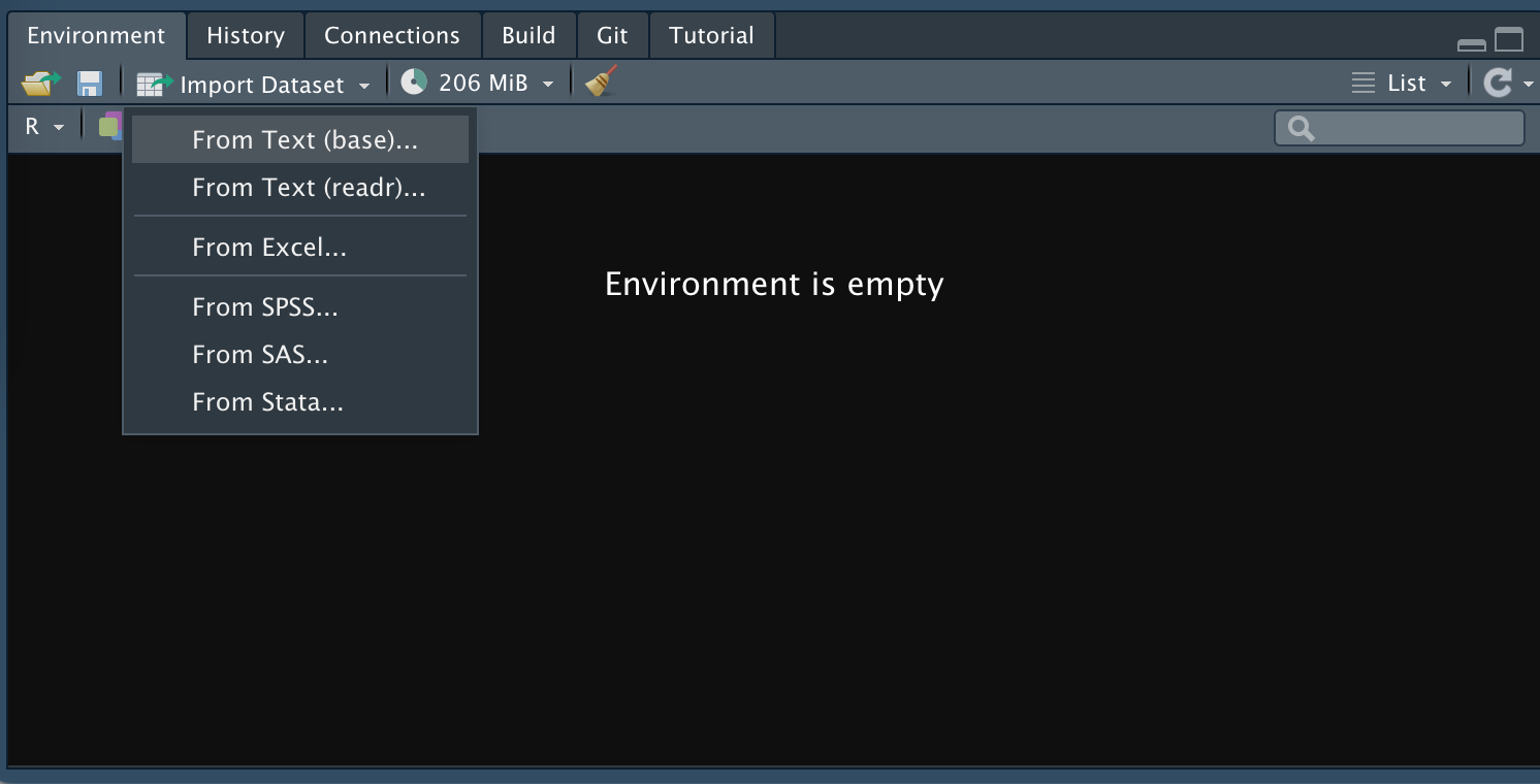
In the environment window on the right, click “Import Dataset” -> “From Text File” -> select the file, and select the plausible options (eg. header, missing value, and whether strings (characters) will be treated as factors). In this example, we are going to treat the first column as the row names.

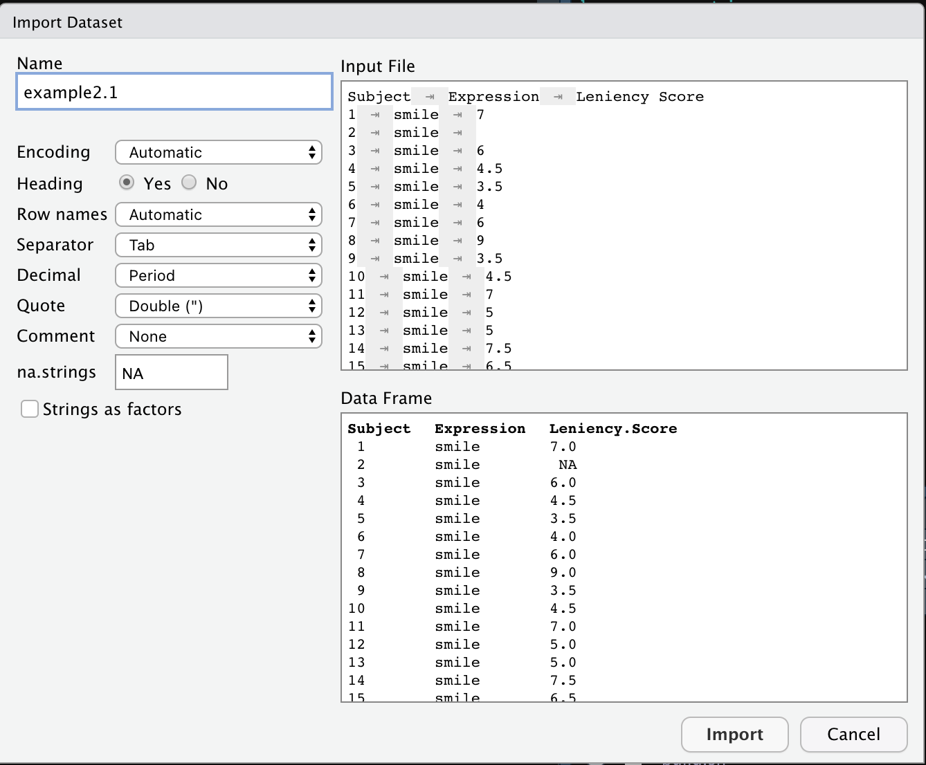
The imported data file example2.1 is saved as a data frame object in the environment. This data frame consists of 30 observations of 2 variables.

Or, the .txt files can be imported to R using the read.table() function. The argument header = TRUE indicates that the first row of the .txt file should be imported as the variable names. The argument row.names = TRUE indicates that the first column should be imported as the row names.

example2.1 <- read.table("example2.1.txt", header = TRUE, row.names = 1)

class(example2.1)
nrow(example2.1)
ncol(example2.1)

To see the first six observations of this data frame:

head(example2.1)

##   Expression LeniencyScore
## 1      smile           7.0
## 2      smile            NA
## 3      smile           6.0
## 4      smile           4.5
## 5      smile           3.5
## 6      smile           4.0

We can refer to a column/variable by $ or [].

example2.1$Expression

##  [1] "smile"   "smile"   "smile"   "smile"   "smile"   "smile"   "smile"  
##  [8] "smile"   "smile"   "smile"   "smile"   "smile"   "smile"   "smile"  
## [15] "smile"   "smile"   "neutral" "neutral" "neutral" "neutral" "neutral"
## [22] "neutral" "neutral" "neutral" "neutral" "neutral" "neutral" "neutral"
## [29] "neutral" "neutral"

example2.1[, 1]

##  [1] "smile"   "smile"   "smile"   "smile"   "smile"   "smile"   "smile"  
##  [8] "smile"   "smile"   "smile"   "smile"   "smile"   "smile"   "smile"  
## [15] "smile"   "smile"   "neutral" "neutral" "neutral" "neutral" "neutral"
## [22] "neutral" "neutral" "neutral" "neutral" "neutral" "neutral" "neutral"
## [29] "neutral" "neutral"

Let’s assign a simpler name for the second variable LeniencyScore.

len <- example2.1$LeniencyScore
len

##  [1] 7.0  NA 6.0 4.5 3.5 4.0 6.0 9.0 3.5 4.5 7.0 5.0 5.0 7.5 6.5 2.0 4.0 4.0 3.0
## [20] 6.0 4.5 2.0 6.0 3.0 3.0 4.5 8.0 4.0 5.0 2.5

Before directly jumping into more sophisticated data analysis, it is always a good practice to start with some descriptive statistics. The arguments na.rm = T omits the missing values, so that the numerical mean, median, and variance of the object is available.

summary(example2.1$Expression)

##    Length     Class      Mode 
##        30 character character

summary(example2.1$LeniencyScore)

##    Min. 1st Qu.  Median    Mean 3rd Qu.    Max.    NA's 
##   2.000   3.500   4.500   4.845   6.000   9.000       1

table(example2.1$LeniencyScore)   #list all values and frequencies

## 
##   2 2.5   3 3.5   4 4.5   5   6 6.5   7 7.5   8   9 
##   2   1   3   2   4   4   3   4   1   2   1   1   1

table(example2.1$Expression)

## 
## neutral   smile 
##      14      16

mean(len, na.rm = TRUE) #average

## [1] 4.844828

median(len, na.rm = TRUE)

## [1] 4.5

var(len, na.rm = TRUE)  #variance

## [1] 3.23399

sd(len, na.rm  = TRUE)   #standard deviation, sqrt(var)

## [1] 1.79833

Another good way to explore the data set is to draw plots.

hist(len)

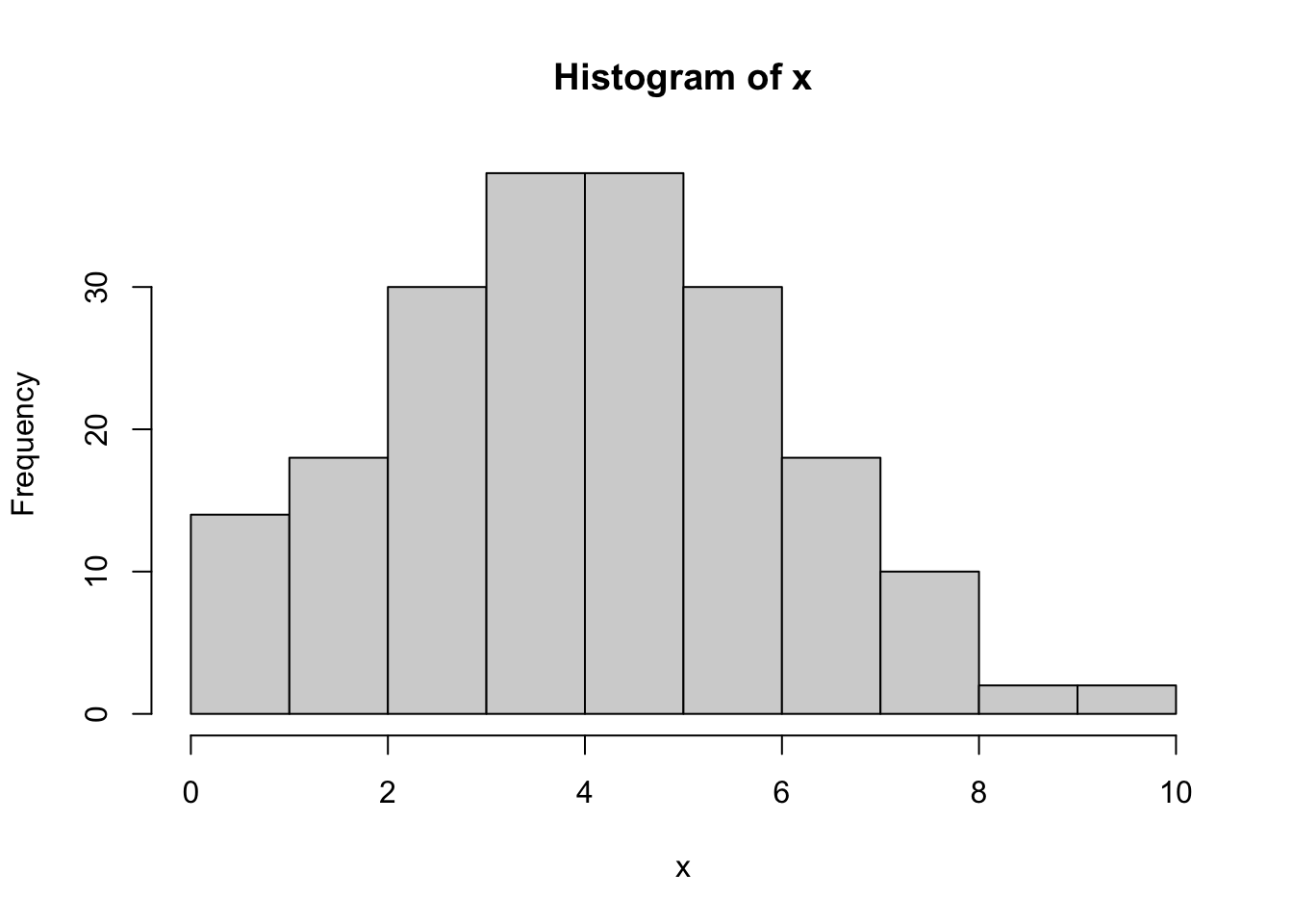
The hist() function plots the counts in the cells with equi-spaced breaks. The height of a rectangle is proportional to the number of points falling into the cell.

boxplot(len)

The boxplot() function plots the box and whisker plot. It displays the five-number summary of a set of data. These are the minimum, the maximum, the first/third quartiles, and the median.

boxplot(len ~ example2.1$Expression)

Running boxplot(len ~ example2.1$Expression) will split the len vector into groups according to the grouping variable example2.1$Expression and plot the box plots for each group (i.e., ‘neutral’ and ‘smile’).

You can create a data frame by combining vectors. First, create the vectors, or variables we want to include in our data frame.

Item <- c("milk", "cold brew coffee", "dishliquid", "avocado")
Unit_price <- c(3.9, 6, 1.5, 1)
Quantity <- c(1, 1, 1, 4)
Cost <- Unit_price * Quantity

Use data.frame() to combine the created vectors to construct a data frame named Receipt.

Receipt <- data.frame(Item, Unit_price, Quantity, Cost)
Receipt

##               Item Unit_price Quantity Cost
## 1             milk        3.9        1  3.9
## 2 cold brew coffee        6.0        1  6.0
## 3       dishliquid        1.5        1  1.5
## 4          avocado        1.0        4  4.0

3.3 Your turn

Create a 4 $\times$ 4 matrix named B that looks like:

\[\begin{pmatrix} 1 & 2 & 3 & 4\\ 5 & 6 & 7 & 8\\ 9 & 10 & 11 & 12\\ 13 & 14 & 15 & 16\\ \end{pmatrix} \]

Extract the element in the $1$st column and the $3$rd row from B.
Extract the third row of B and save it as an object named b3.
From the data set example2.1, extract the first variable and name the object as exp.