Chapter 2 Two-Way Contingency Tables

Contingency tables are data arrays containing counts of observations that are recorded in cross-classifications by a number of discrete factor predictors. They can therefore be seen as summaries of response data where the predictor variables are discrete factors or categorical variables, and where the responses are counts.

2.1 \(2 \times 2\) Tables

In this section we introduce some useful ideas for the more general \(I \times J\) tables discussed in Section 2.2 onwards.

• \(2 \times 2\) tables are very common in biomedical and social sciences. They are particularly useful for binary variables, for example
  • success of a treatment,
  • presence of a characteristic or prognostic factor.

Let \(X\) and \(Y\) denote two categorical binary response variables. A \(2 \times 2\) table¹⁴ may be given as shown in Figure 2.1, where

• \(n_{ij}\) denotes the observed cell frequency in cell \((i,j)\).
• \(n_{i+} = n_{i1} + n_{i2}\) is the marginal frequency for row \(i = 1,2\).
• \(n_{+j} = n_{1j} + n_{2j}\) is the marginal frequency for column \(j = 1,2\).
• \(n_{++} = n_{1+} + n_{2+} = n_{+1} + n_{+2}\) is the total number of observations in the dataset¹⁵.

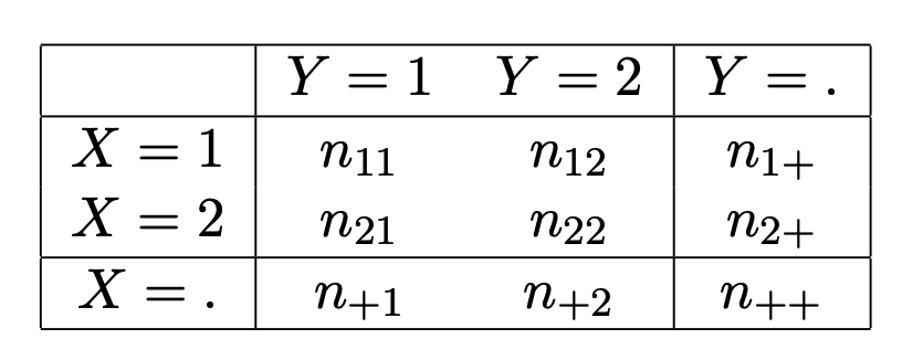
Figure 2.1: Generic 2 x 2 contingency table of counts.

2.1.1 Example

Table 2.1 shows a sample of \(n_{++} = 3213\) collected in the period 1980-1983 in the St. Louis Epidemiological Catchment Area Survey and cross-classified according to regular smoking habit (rows) and major depressive disorder (columns) (Covey, Glassman, and Stetner (1990)).

Question

• Is there a relation between cigarette smoking and major depressive disorder?

Table 2.1: Survey respondents cross-classified by smoking habit and major depressive disorder.

	Depression: Yes	No	Sum
Ever Smoked: Yes	144	1729	1873
Ever Smoked: No	50	1290	1340
Sum	194	3019	3213

2.1.2 Sampling Schemes

Consider the generic \(2 \times 2\) contingency table in Figure 2.1.
Before being observed, the counts \(N_{ij}\) are variables to be sampled from a particular distribution, with \(n_{ij}\) then forming a realisation from the sampling scheme.

Important: It is important to understand the implication of different sampling distributions. Each one represents a different sampling scheme or data collection mechanism, these being determined by the experiment being performed (which is likely being driven by a hypothesis to be tested).

Here we provide a brief illustration of what we mean - these will be considered in greater detail in Section 2.3.

2.1.2.1 Poisson Sampling Scheme

Poisson sampling describes the scenario where the dataset (\(n_{ij}\)) is collected (sampled) independently in a given spatial, temporal, or other interval.

Then, \(n_{ij}\) is a realisation of a Poisson random variable \[\begin{equation} N_{ij} \sim Poi(\lambda_{ij}) \end{equation}\] so that \[\begin{equation} P(N_{ij}=n_{ij}) = \frac{\exp(-\lambda_{ij}) \lambda_{ij}^{n_{ij}}}{n_{ij}!} \end{equation}\] where \(\lambda_{ij}\) are the rate parameters.

2.1.2.1.1 Example

Consider the survey data in Table 2.1. We can see that this survey follows a Poisson sampling scheme if it involved questioning people randomly over a fixed timeframe. We do not how many people will be questioned in total beforehand (perhaps as many as possible), and so each compartment now represents an independent Poisson count result (in the sense that we could have counted any of those compartments separately or only and got the same result).

2.1.2.2 Multinomial Sampling Scheme

What if \(n_{++}\) is fixed (that is, predetermined)?

Well, then we have that \[\begin{equation} (N_{11}, N_{12}, N_{21}, N_{22}) \sim Mult(n_{++}, (\pi_{11}, \pi_{12}, \pi_{21}, \pi_{22})) \end{equation}\] so that \[\begin{equation} P((N_{11}, N_{12}, N_{21}, N_{22}) = (n_{11}, n_{12}, n_{21}, n_{22}) | N_{++} = n_{++}) = \frac{n_{++}!}{\prod_{i,j}n_{ij}!} \prod_{i,j} \pi_{ij}^{n_{ij}} \end{equation}\] where \(\pi_{ij} = P(X=i, Y=j)\) is the theoretical probability of sampling someone in compartment \((i,j)\) from the represented population. The probability vector \(\boldsymbol{\pi}=(\pi_{11}, \pi_{12}, \pi_{21}, \pi_{22})\) is the joint distribution of \(X\) and \(Y\).

2.1.2.2.1 Example

The data in Table 2.2 represents a hypothetical crossover trial.
One fixed sample of patients of size \(n_{++}=100\) is considered and they receive a low dose and then a high dose of a particular treatment, one week apart. A pair of responses is available for each patient and Table 2.2 cross-classifies these responses, reporting the number of treatments for which both treatments were successful, both failed, or one succeeded and the other failed. Notice that each patient has to belong to one of the four compartments, and given that there is a fixed sample of 100 patients, means that the setup of this experiment has resulted in a multinomial sampling procedure.

Table 2.2: Hypothetical data of a crossover trial comparing low and high dose treatments on a sample of 100 patients.

	Low Dose: Success	Failure	Sum
High Dose: Success	62	18	80
High Dose: Failure	8	12	20
Sum	70	30	100

2.1.2.3 Product Binomial Sampling Scheme

We now assume the marginal row sizes \(n_{1+}, n_{2+}\) are fixed. In this case \[\begin{align} N_{11} & \sim Bin(n_{1+}, \pi_{11}) \\ N_{21} & \sim Bin(n_{2+}, \pi_{21}) \end{align}\] so that \[\begin{align} P(N_{11} = n_{11} | N_{1+} = n_{1+}) & = \binom{n_{1+} }{ n_{11}} \pi_{11}^{n_{11}} \pi_{12}^{n_{12}} \\ P(N_{21} = n_{21} | N_{2+} = n_{2+}) & = \binom{n_{2+} }{ n_{21}} \pi_{21}^{n_{21}} \pi_{22}^{n_{22}} \end{align}\] and \[\begin{align} \pi_{12} & = 1 - \pi_{11} \\ \pi_{22} & = 1 - \pi_{21} \\ N_{12} & = n_{1+} - N_{11} \\ N_{22} & = n_{2+} - N_{12} \end{align}\]

2.1.2.3.1 Example

The data in Table 2.3 are similar to that of Table 2.2, however the experiment is designed differently. Instead of a crossover trial, where each patient is given both treatments, the sample of \(100\) patients is now divided equally into subsamples of size \(50\). The patients in each subsample either receive a high or low dose of treatment, and the result is recorded. Note that the row sums are fixed in this case, and so this would correspond to a product multinomial sampling scheme.

Table 2.3: Hypothetical data from two independent samples of low and high dose treatments.

	Response: Success	Failure	Sum
Dose: High	41	9	50
Dose: Low	37	13	50
Sum	78	22	100

2.1.3 Odds and Odds Ratio

2.1.3.1 Odds

Given a generic success probability \(\pi_A\) of event \(A\) (a binary response), we are often interested in the odds of success of an event \(A\), given by \[\begin{equation} \omega_A = \frac{\pi_A}{1-\pi_A} \end{equation}\]

Interpretation: \[\begin{eqnarray} \omega_A = 1 \implies \pi_A = 1-\pi_A & \implies & \textrm{success is equally likely as failure} \nonumber \\ \omega_A > 1 \implies \pi_A > 1-\pi_A & \implies & \textrm{success is more likely than failure} \nonumber \\ \omega_A < 1 \implies \pi_A < 1-\pi_A & \implies & \textrm{success is less likely than failure} \nonumber \end{eqnarray}\]

Question: What does an odds of 2 mean relative to success probability \(\pi_A\)?

2.1.3.2 Odds Ratio

If \(\pi_A\) and \(\pi_B\) are the success probabilities for two events \(A\) and \(B\), then their odds ratio is defined as \[\begin{equation} r_{AB} = \frac{\omega_A}{\omega_B} = \frac{\pi_A/(1-\pi_A)}{\pi_B/(1-\pi_B)} \end{equation}\]

\(r_{AB}\) can be interpreted as the (multiplicative) difference in the odds (relative chance) of success to failure between event A and event B. Therefore: \[\begin{eqnarray} r_{AB} = 1 & \implies & \omega_A = \omega_B \nonumber \\ & \implies & \textrm{the relative chance of success to failure of $A$ is equal to that of $B$} \nonumber \\ r_{AB} > 1 & \implies & \omega_A > \omega_B \nonumber \\ & \implies & \textrm{the relative chance of success to failure of $A$ is greater than that of $B$} \nonumber \\ r_{AB} < 1 & \implies & \omega_A < \omega_B \nonumber \\ & \implies & \textrm{the relative chance of success to failure of $A$ is less than that of $B$} \nonumber \end{eqnarray}\]

Odds ratios are typically more informative for the comparison of \(\pi_A\) and \(\pi_B\) than looking at their difference \(\pi_A - \pi_B\) or their relative risk \(\pi_A / \pi_B\).

2.1.3.3 Odds Ratio for a \(2 \times 2\) Contingency Table

In terms of the joint distribution of a \(2 \times 2\) contingency table, the odds ratio \(r_{12}\) is given by¹⁶ \[\begin{equation} r_{12} = \frac{\pi_{11}/\pi_{12}}{\pi_{21}/\pi_{22}} = \frac{\pi_{11}/\pi_{21}}{\pi_{12}/\pi_{22}} = \frac{\pi_{11} \pi_{22}}{\pi_{12} \pi_{21}} \end{equation}\] and is a (multiplicative) measure of

• the difference in the odds (relative chance) of \(Y=1\) to \(Y=2\) between \(X=1\) and \(X=2\); equivalently
• the difference in the odds (relative chance) of \(X=1\) to \(X=2\) between \(Y=1\) and \(Y=2\).

Therefore: \[\begin{eqnarray} r_{12} = 1 & \implies & \pi_{11}/\pi_{12} = \pi_{21}/\pi_{22} \nonumber \\ & \implies & \textrm{the relative chance of $Y=1$ to $Y=2$ is the same given $X=1$ or $X=2$} \nonumber \\ & \implies & \pi_{11}/\pi_{21} = \pi_{12}/\pi_{22} \nonumber \\ & \implies & \textrm{the relative chance of $X=1$ to $X=2$ is the same given $Y=1$ or $Y=2$} \nonumber \end{eqnarray}\] \[\begin{eqnarray} r_{12} > 1 & \implies & \pi_{11}/\pi_{12} > \pi_{21}/\pi_{22} \nonumber \\ & \implies & \textrm{the relative chance of } Y=1 \textrm{ to } Y=2 \textrm{ given } X=1 \textrm{ is greater than given } X=2 \nonumber \\ & \implies & \pi_{11}/\pi_{21} > \pi_{12}/\pi_{22} \nonumber \\ & \implies & \textrm{the relative chance of } X=1 \textrm{ to } X=2 \textrm{ given } Y=1 \textrm{ is greater than given } Y=2 \nonumber \end{eqnarray}\] \[\begin{eqnarray} r_{12} < 1 & \implies & \pi_{11}/\pi_{12} < \pi_{21}/\pi_{22} \nonumber \\ & \implies & \textrm{the relative chance of } Y=1 \textrm{ to } Y=2 \textrm{ given } X=1 \textrm{ is less than given } X=2 \nonumber \\ & \implies & \pi_{11}/\pi_{21} < \pi_{12}/\pi_{22} \nonumber \\ & \implies & \textrm{the relative chance of } X=1 \textrm{ to } X=2 \textrm{ given } Y=1 \textrm{ is less than given } Y=2 \nonumber \end{eqnarray}\]

2.1.3.4 Sample Odds Ratio

The sample odds ratio is \[\begin{equation} \hat{r}_{12} = \frac{p_{11}p_{22}}{p_{12} p_{21}} = \frac{n_{11}n_{22}}{n_{12} n_{21}} \end{equation}\] where \(p_{ij} = n_{ij}/n_{++}\) is the sample proportion in class \((i,j)\).

2.1.3.5 Example

Consider the data in Table 2.3.

• The sample proportions of success for high and low dose of treatment are \(p_{H} = \frac{41}{50}\), and \(p_{L} = \frac{37}{50}\) respectively.

• The overall proportions are \(p_{11} = \frac{41}{100}\), and \(p_{21} = \frac{37}{100}\).

• The sample odds of success assuming high dose is \[\begin{equation} \frac{p_H}{1-p_H} = \frac{41/50}{9/50} = \frac{41}{9} \approx 4.556 \end{equation}\]

• Incidentally (and unsurprisingly), using the overall proportion values: \[\begin{equation} \frac{p_{11}}{p_{12}} = \frac{41/100}{9/100} = \frac{41}{9} \end{equation}\] yields the same value.

• The sample odds of success assuming low dose is \[\begin{equation} \frac{p_L}{1-p_L} = \frac{37}{13} \approx 2.846 \end{equation}\]

• The sample odds ratio is given by \[\begin{equation} \frac{n_{11}n_{22}}{n_{12}n_{21}} = \frac{41 \times 13}{9 \times 37} = \frac{533}{333} \approx 1.601 \end{equation}\]

2.2 \(I \times J\) Tables

• Let \(X\) and \(Y\) denote two categorical response variables (also called classifiers).
• \(X\) has \(I\) categories and \(Y\) has \(J\) categories.
• Classifications of subjects on both variables have \(IJ\) possible combinations.

2.2.1 Table of Counts

The \(I \times J\) contingency table¹⁷ of observed frequencies \(n_{ij}\) for \(X\) and \(Y\) is the rectangular table

• which has \(I\) rows for categories of \(X\) and \(J\) columns for categories of \(Y\),
• whose cells represent the \(IJ\) possible outcomes of the responses \((X,Y)\),
• which displays \(n_{ij}\), the observed number of outcomes \((i,j)\) in each case.

Such a table is shown as given in Figure 2.2.

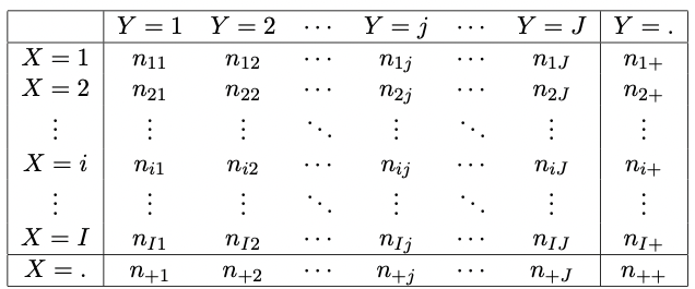
Figure 2.2: Generic I x J contingency table of \(X\) and \(Y\) displaying the observed number of outcomes \((X=i,Y=j)\).

Similar to \(2 \times 2\) tables, we have that

• \(n_{ij}\) denotes the observed number (or counts, frequency) of outcomes \((i,j)\)¹⁸.
• \(n_{i+} = \sum_j n_{ij}\) is the marginal frequency of outcomes \(X=i\) regardless of the outcome of \(Y\).
• \(n_{+j} = \sum_i n_{ij}\) is the marginal frequency of outcomes \(Y=j\) regardless of the outcome of \(X\).
• \(n_{++} = \sum_{i,j} n_{ij}\) is the observed total number of observations in the dataset.

2.2.2 Table of Theoretical Probabilities

Similar to the \(2 \times 2\) case, we define

• \(\pi_{ij} = P(X=i, Y=j)\) to be the theoretical probability of getting outcome \((i,j)\).

We also define

• \(\pi_{i+} = \sum_j \pi_{ij}\) to be the marginal probability of getting an outcome \(X=i\) regardless of the outcome of \(Y=j\).
• \(\pi_{+j} = \sum_i \pi_{ij}\) to be the marginal probability of getting an outcome \(Y=j\) regardless of the outcome of \(X=i\).
• \(\pi_{++} = \sum_{i,j} \pi_{ij} = 1\)

One can tabulate the distribution \(\pi_{ij} = P(X=i, Y=j)\) of responses \((X,Y)\) as in the classification given in Figure 2.3.

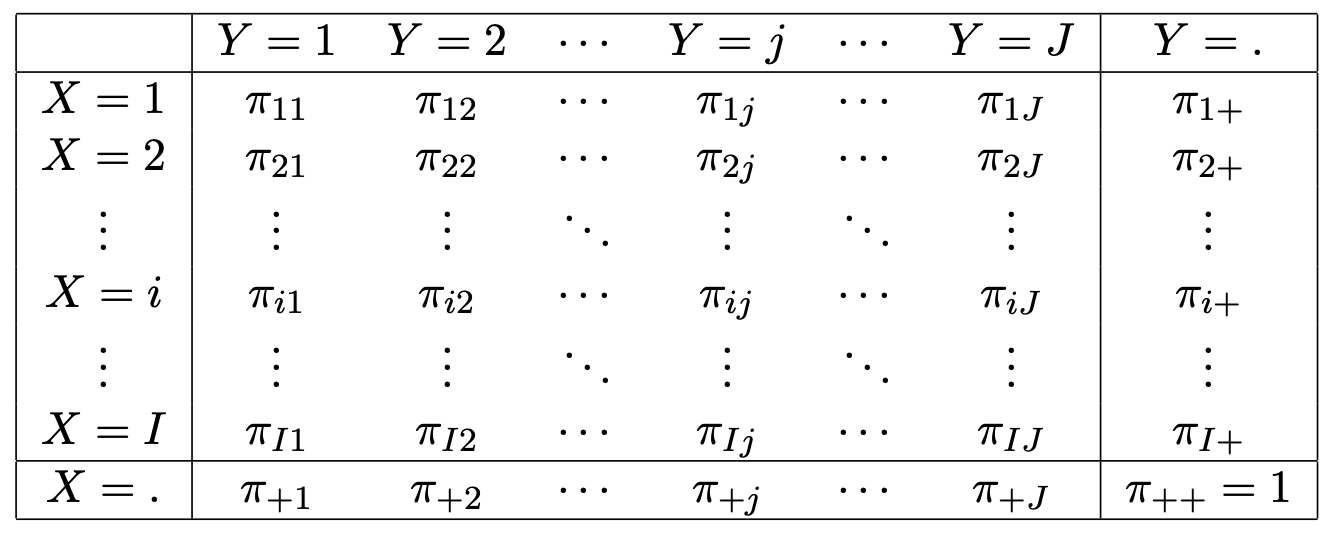
Figure 2.3: Generic IJ contingency table of the theoretical probability distribution of responses.

2.2.3 Additional Tables

In a similar manner, a contingency table can display the following quantities

• \(p_{ij} = \frac{n_{ij}}{n_{++}}\) - the observed proportion of outcomes \((i,j)\).
• \(\mu_{ij}\) - the expected number of outcomes \((i,j)\).
• \(N_{ij}\) - the variable number of outcomes \((i,j)\) (before the observations are collected).

2.2.4 Conditional Probabilities

Contingency tables can also display the following conditional quantities:

• \(\pi_{i|j} = \frac{\pi_{ij}}{\pi_{+j}} = P(X=i|Y=j)\) - the conditional probability of getting an outcome \(X=i\) given that the outcome \(Y=j\).
• \(\pi_{j|i} = \frac{\pi_{ij}}{\pi_{i+}} = P(Y=j|X=i)\) - the conditional probability of getting an outcome \(Y=j\) given that the outcome \(X=i\).
• \(p_{i|j} = \frac{p_{ij}}{p_{+j}} = \frac{n_{ij}}{n_{+j}}\) - the observed proportion of the outcomes with \(Y=j\) for which \(X=i\).
• \(p_{j|i} = \frac{p_{ij}}{p_{i+}} = \frac{n_{ij}}{n_{i+}}\) - the observed proportion of the outcomes with \(X=i\) for which \(Y=j\).

Two schematics of tables representing the conditional probabilities \(\pi_{j|i}\), and conditional proportions \(p_{j|i}\) of the outcomes \(Y=j\), given that \(X=i\) (that is, conditioning on the rows) are given by the Tables in Figures 2.4 and 2.5.

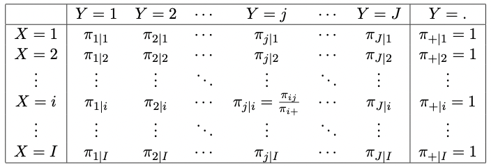
Figure 2.4: A generic IJ table displaying the conditional probabilities of the outcome Y given outcome X.

Figure 2.5: A generic IJ table displaying the conditional proportions of the outcome Y given outcome X.

2.3 Sampling Schemes

We here go into a bit more detail on some of the sampling schemes introduced in Section 2.1.2 for \(2 \times 2\) tables.

Remember that it is important to understand the implication of different sampling distributions. Each one represents a different sampling scheme or data collection mechanism, these being determined by the experiment being performed (which is likely being driven by a hypothesis to be tested).

2.3.1 Poisson Sampling Scheme

As discussed in Section 2.1.2.1, Poisson sampling describes the scenario where the dataset (\(n_{ij}\)) is collected (sampled) independently in a given spatial, temporal, or other interval.

Then, \(n_{ij}\) is a realisation of a Poisson random variable \[\begin{equation} N_{ij} \sim Poi(\lambda_{ij}) \end{equation}\] so that \[\begin{equation} P(N_{ij}=n_{ij}) = \frac{\exp(-\lambda_{ij}) \lambda_{ij}^{n_{ij}}}{n_{ij}!} \end{equation}\] where \(\lambda_{ij}\) are the rate parameters.

2.3.1.1 Mean and Variance

We have that \[\begin{align} {\mathrm E}[N_{ij}] & = \lambda_{ij} \\ {\mathrm{Var}}[N_{ij}] & = \lambda_{ij} \end{align}\] for \(i = 1,...,I\) and \(j = 1,...,J\).

2.3.1.2 Likelihood

The likelihood is \[\begin{equation} L(\boldsymbol{\lambda}) = \prod_{i,j} \frac{\exp(-\lambda_{ij}) \lambda_{ij}^{n_{ij}}}{n_{ij}!} \propto \exp ( - \sum_{i,j} \lambda_{ij} ) \prod_{i,j} \lambda_{ij}^{n_{ij}} \tag{2.1} \end{equation}\] where \(\boldsymbol{\lambda} = (\lambda_{11}, \lambda_{12},...,\lambda_{IJ})^T\).

2.3.2 Multinomial Sampling Scheme

The Multinomial sampling scheme describes the scenario where the dataset \((n_{ij})\) is collected (sampled) independently given that the total sample size \(n_{++}\) is fixed/predetermined. Then \(\boldsymbol{n} = (n_{11}, n_{12},...,n_{IJ})^T\) is a realisation of a Multinomial random variable¹⁹ \[\begin{equation} \boldsymbol{N} \sim Mult(n_{++}, \boldsymbol{\pi}) \end{equation}\] where \(\boldsymbol{N} = (N_{11}, N_{12},...,N_{IJ})^T\) and \(\boldsymbol{\pi} = (\pi_{11}, \pi_{12},...,\pi_{IJ})^T\), so that \[\begin{equation} P(\boldsymbol{N} = \boldsymbol{n} | N_{++} = n_{++}) = \frac{n_{++}!}{\prod_{i,j}n_{ij}!} \prod_{i,j} \pi_{ij}^{n_{ij}} \end{equation}\]

2.3.2.1 Mean and Variance

We have that \[\begin{align} {\mathrm E}[\boldsymbol{N}] & = n_{++} \boldsymbol{\pi} \\ {\mathrm{Var}}[\boldsymbol{N}] & = n_{++} (\textrm{diag}(\boldsymbol{\pi}) - \boldsymbol{\pi}\boldsymbol{\pi}^T) \end{align}\] for \(i = 1,...,I\) and \(j = 1,...,J\).

2.3.2.2 Likelihood

The likelihood is \[\begin{equation} L(\boldsymbol{\pi}) = P(\boldsymbol{N} = \boldsymbol{n}|N_{++} = n_{++}) = \frac{n_{++}!}{\prod_{i,j} n_{ij}!} \prod_{i,j} \pi_{ij}^{n_{ij}} \propto \prod_{i,j} \pi_{ij}^{n_{ij}} \tag{2.2} \end{equation}\] as \(n_{++}\) is predetermined and fixed. Notice that since \(\mu_{ij} = n_{++} \pi_{ij}\), we have that \[\begin{equation} L(\boldsymbol{\pi}) = \prod_{i,j} \left( \frac{\mu_{ij}}{n_{++}} \right)^{n_{ij}} \propto \prod_{i,j} \mu_{ij}^{n_{ij}} \tag{2.3} \end{equation}\]

2.3.3 Product Multinomial Sampling Scheme

The Product Multinomial sampling scheme describes the scenario where the sample \((n_{ij})\) is collected randomly, given that the marginal row sizes \(n_{i+}\) are fixed/predetermined for \(i=1,...,I\). Then \((n_{i1},...,n_{iJ})\) is a realisation of the Multinomial random variable \[\begin{equation} (N_{i1},...,n_{iJ}) \sim Mult(n_{i+}, \boldsymbol{\pi}_i^*) \end{equation}\] where \(\boldsymbol{\pi}_i^\star = (\pi_{1|i},...,\pi_{J|i})\) for \(i=1,...,I\), so that \[\begin{equation} P(\boldsymbol{N} = \boldsymbol{n} | \boldsymbol{N}_{i+} = \boldsymbol{n}_{i+}) = \prod_i \left[ \frac{n_{i+}!}{\prod_{j}n_{ij}!} \prod_{j} \pi_{j|i}^{n_{ij}} \right] \end{equation}\] where \(\boldsymbol{N}_{i+} = (N_{1+},...,N_{I+})\).

2.3.3.1 Likelihood

The likelihood is \[\begin{equation} L(\boldsymbol{\pi}) = \prod_i \left[ \frac{n_{i+}!}{\prod_{j} n_{ij}!} \prod_{j} \pi_{j|i}^{n_{ij}} \right] \propto \prod_{i} \prod_{j} \pi_{j|i}^{n_{ij}} = \prod_{i,j} \left( \frac{\pi_{ij}}{\pi_{i+}} \right)^{n_{ij}} \propto \prod_{i,j} \pi_{ij}^{n_{ij}} \end{equation}\] since \(\pi_{i+}\) is determined and fixed by the fact that \(n_{i+}\) is determined and fixed. Notice that since \(\mu_{ij} = n_{++} \pi_{ij}\), we have that \[\begin{equation} L(\boldsymbol{\pi}) \propto \prod_{i,j} \left( \frac{\mu_{ij}}{n_{++}} \right)^{n_{ij}} \propto \prod_{i,j} \mu_{ij}^{n_{ij}} \tag{2.4} \end{equation}\]

2.3.4 Inferential Equivalence

Proposition: The three sampling schemes in Sections 2.3.1, 2.3.2 and 2.3.3 lead to the same MLE.

Proof: By Equations (2.3) and (2.4), it is clear for the Multinomial sampling scheme and the product Multinomial sampling scheme.

Now, consider Equation (2.1). Upon observing the sample, we can condition on the total sample size \(n_{++}\). Then, using the result of Section 1.4.3.4, we have that \[\begin{equation} L(\boldsymbol{\lambda}|n_{++}) = \frac{n_{++}!}{\prod_{i,j} (n_{ij}!)} \prod_{i,j} \left( \frac{\lambda_{ij}}{\lambda} \right)^{n_{ij}} \propto \prod_{i,j} \pi_{ij}^{n_{ij}} \propto \prod_{i,j} \mu_{ij}^{n_{ij}} \end{equation}\]

Although we have inferential equivalence in terms of MLEs, the different sampling schemes are still important as they are guided by, and inform us about, the data collection mechanism and experiment being performed (and perhaps any hypothesis being tested).

2.3.5 Fixed Row and Column Sums

A final scenario we have not yet considered is that where sample \((n_{ij})\) is collected randomly given that the marginal counts \(n_{i+}\) and \(n_{+j}\) are fixed and predetermined before the experiment was performed. It is actually quite unusual to be in such a situation, and the probability distributions representing possible configurations are more challenging to represent. We will consider specific scenarios only.²⁰

2.3.6 What now?

So, we have introduced contingency tables as a means of presenting cross-classification data of two categorical variables. We have explained that different experimental scenarios naturally lead to different sampling schemes.

Now what?

• We may wish to test the homogeneity of \(Y\) given \(X\). For example, in Table 2.3, is the distribution of Response (Y) the same regardless of dose level (X) (Section 2.4.3)?

• We may wish to test independence (correlation, association) of \(X\) and \(Y\). For example, in Table 2.1, is there a correlation between cigarette smoking and major depressive disorder, or are they uncorrelated (Section 2.4.4)?

• If there is an association between two variables, we may wish to understand more about the strength of association, and what elements of the table are driving this conclusion.

• We may wish to understand more about how we can draw conclusions from the data using Odds Ratios (less clear for \(I\times J\) tables than \(2 \times 2\) tables).

• Maybe we need ways of presenting our results to non-experts (visualisation - see Practical 1).

• Maybe we want to do all of the above considering more than two categorical variables (Section 3).

2.4 Chi-Square Test

The chi-square goodness-of-fit test can be used to determine whether a given sample is consistent with a (specified) hypothesised distribution. Thus, the term goodness-of-fit implies how well the distributional assumption fits the data. This test was initially developed by Karl Pearson in 1900 for categorical data. We will utilise this test in the context of contingency tables to test for homogeneity and independence²¹.

Suppose data consists of a random sample of \(m\) independent observations which are classified into \(k\) mutually exclusive and exhaustive categories. The number of observations falling into category \(j\), for \(j = 1,...,k\), is called the observed frequency of that category, and denoted by \(O_j\).

We wish to test a statement about the unknown probability distribution \(\boldsymbol{\pi} = (\pi_1,...,\pi_k)\) of the random variable being observed, where \(\pi_j\) is the theoretical probability of an observation in category \(j\). We denote the specified probabilities under our hypothesised distribution as \(\boldsymbol{\pi_0} = (\pi_{0,1},...,\pi_{0,k})\) Thus, the null and alternative hypotheses are \[\begin{align} \mathcal{H}_0: & \pi_j = \pi_{0,j}, \qquad j = 1,...,k \\ \mathcal{H}_1: & \pi_j \neq \pi_{0,j}, \qquad \textrm{for any } j = 1,...,k \end{align}\]

2.4.1 The Chi-Square Test Statistic

The Chi-Square goodness-of-fit test statistic is \[\begin{equation} X^2 = \sum_{j=1}^k \frac{(O_j - E_j)^2}{E_j} \tag{2.5} \end{equation}\] where \(O_j\) are the observed frequencies, \(E_j = m \pi_{0,j}\) are the expected frequencies, and \(m = \sum_{j=1}^k O_j\) is the total sample size.

The chi-square test statistic is based on the difference between the expected and observed frequencies. The larger the differences between the expected and observed frequencies, the larger the chi-square test statistic value will be, hence providing evidence against the null hypothesis.

2.4.2 Asymptotic Distribution of \(X^2\)

Proposition: For large \(m\), we have that, under \(\mathcal{H}_0\): \[\begin{equation} X^2 \sim \chi^2_{k-1} \end{equation}\] where \(k\) is the number of categories.

Consequence: We reject \(\mathcal{H}_0\) at significance level \(\alpha\) if \[\begin{equation} X^2 \geq \chi^{2, \star}_{k-1, \alpha} \end{equation}\] where \(\chi^{2, \star}_{k-1, \alpha}\) is the \((1-\alpha)\)-quantile of the \(\chi^2_{k-1}\)-distribution.

Proof: Each observation \(i = 1,...,m\) can be viewed as an observation of random variable \(\boldsymbol{X}_i\), these being \(m\) independent variables drawn from \[\begin{equation} \boldsymbol{X}_i \sim Mult(1, \boldsymbol{\pi}) \end{equation}\] where \(\boldsymbol{\pi} = (\pi_1,...,\pi_k)\) is the vector of probabilities that any randomly selected observation belongs to each category. Each \(\boldsymbol{X}_i\) consists of exactly \(k-1\) zeroes and a single one, where the one is in the component of the observed category at trial \(i\).

Under this view, we have that \[\begin{align} E_j & = m \pi_j \\ O_j & = m \bar{X}_{j} \end{align}\] where \(\bar{\boldsymbol{X}} = \frac{1}{m} \sum_{i=1}^m \boldsymbol{X}_i\), so that \[\begin{equation} X^2 = m \sum_{j=1}^k \frac{(\bar{X}_{j} - \pi_j)^2}{\pi_j} \end{equation}\]

We have that (using the multinomial results of Section 1.4.3.1) \[\begin{align} {\mathrm{Var}}[X_{ij}] & = \pi_j(1-\pi_j) \\ {\mathrm{Cov}}[X_{ij},X_{il}] & = -\pi_j \pi_l, \qquad j \neq l \end{align}\] and that \(\boldsymbol{X}_i\) has covariance matrix \[\begin{equation} \Sigma = \left( \begin{array}{cccc} \pi_1(1-\pi_1) & -\pi_1 \pi_2 & \cdots & -\pi_1 \pi_k \\ -\pi_2 \pi_1 & \pi_2(1-\pi_2) & \cdots & -\pi_2 \pi_k \\ \vdots & & \ddots & \vdots \\ -\pi_k \pi_1 & -\pi_k \pi_2 & \cdots & \pi_k(1-\pi_k) \end{array} \right) \end{equation}\]

Since \({\mathrm E}[\boldsymbol{X}_i] = \boldsymbol{\pi}\), the CLT (Section 1.4.6) implies that \[\begin{equation} \sqrt{m} (\bar{\boldsymbol{X}}_m - \boldsymbol{\pi}) \stackrel{d}{\rightarrow} {\mathcal N}_k(\boldsymbol{0}, \Sigma) \end{equation}\] Note that the sum of the \(j^\textrm{th}\) row of \(\Sigma\) is \(\pi_j - \pi_j(\pi_1 + \cdots + \pi_k) = 0\), hence the sum of the rows of \(\Sigma\) is the zero vector, and thus \(\Sigma\) is not invertible.

Let \(\boldsymbol{Y}_i = (X_{i,1},...,X_{i,k-1})\), with covariance matrix \(\Sigma^\star\) being the upper-left \((k-1) \times (k-1)\) submatrix of \(\Sigma\). Similarly, let \(\boldsymbol{\pi}^\star = (\pi_1,...,\pi_{k-1})\).

One may verify that \(\Sigma^\star\) is invertible and that²² \[\begin{equation} (\Sigma^\star)^{-1} = \left( \begin{array}{cccc} \frac{1}{\pi_1} + \frac{1}{\pi_k} & \frac{1}{\pi_k} & \cdots & \frac{1}{\pi_k} \\ \frac{1}{\pi_k} & \frac{1}{\pi_2} + \frac{1}{\pi_k} & \cdots & \frac{1}{\pi_k} \\ \vdots & & \ddots & \vdots \\ \frac{1}{\pi_k} & \frac{1}{\pi_k} & \cdots & \frac{1}{\pi_{k-1}} + \frac{1}{\pi_k} \\ \end{array} \right) \tag{2.6} \end{equation}\]

Furthermore, \(X^2\) can be rewritten as²³ \[\begin{equation} X^2 = m(\bar{\boldsymbol{Y}} - \boldsymbol{\pi}^\star)^T (\Sigma^\star)^{-1} (\bar{\boldsymbol{Y}} - \boldsymbol{\pi}^\star) \tag{2.7} \end{equation}\]

Now, define \[\begin{equation} \boldsymbol{Z}_m = \sqrt{m} (\Sigma^\star)^{-\frac{1}{2}}(\bar{\boldsymbol{Y}} - \boldsymbol{\pi}^\star) \end{equation}\] Then the central limit theorem implies that \[\begin{equation} \boldsymbol{Z}_m \stackrel{d}{\rightarrow} \mathcal{N}_{k-1}(\boldsymbol{0}, I_{k-1}) \end{equation}\] so that \[\begin{equation} X^2 = \boldsymbol{Z}_m^T \boldsymbol{Z}_m \stackrel{d}{\rightarrow} \chi^2_{k-1} \end{equation}\]

2.4.3 Testing Independence

• Variable \(X\) and \(Y\) are independent if \[\begin{equation} P(X=i,Y=j) = P(X=i)P(Y=j), \qquad i = 1,...,I \quad j = 1,...,J \end{equation}\] that is \[\begin{equation} \pi_{ij} = \pi_{i+} \pi_{+j}, \qquad i = 1,...,I \quad j = 1,...,J \end{equation}\]

2.4.3.1 Hypothesis Test

• If we are interested in testing independence²⁴ between \(X\) and \(Y\), then we wish to test with hypotheses as follows: \[\begin{align} \mathcal{H}_0: & \, X \textrm{ and } Y \textrm{ are not associated.} \\ \mathcal{H}_1: & \, X \textrm{ and } Y \textrm{ are associated.} \end{align}\] which we practically do by testing the following: \[\begin{align} \mathcal{H}_0: & \, \pi_{ij} = \pi_{i+} \pi_{+j}, \qquad i = 1,...,I \quad j = 1,...,J \tag{2.8} \\ \mathcal{H}_1: & \, \mathcal{H}_0 \textrm{ is not true.} \end{align}\]

• Notice that the Chi-Square test can be applied to the problem of testing \(\mathcal{H}_0\) above, where the \(k\) mutually exclusive categories are taken to be the \(IJ\) cross-classified possible pairings of \(X\) and \(Y\).

• Under \(\mathcal{H}_0\), we have that \(E_{ij} = n_{++} \pi_{ij} = n_{++} \pi_{i+} \pi_{+j}\).

• However, we do not know \(\pi_{ij}\) or \(\pi_{i+}, \pi_{+j}\), but we can estimate them using ML.

2.4.3.2 Maximum Likelihood

Assume that the sampling distribution has been specified according to the sampling scheme used. Under an assumed relation between \(X\) and \(Y\), ML estimates of \(\{ \pi_{ij} \}\) can be obtained using the method of Lagrange multipliers (see Section 1.4.7).

2.4.3.2.1 ML - no Independence

Consider a Multinomial sampling scheme. We do not assume any independence for \(X\) and \(Y\) . We need to find the MLE of \(\boldsymbol{\pi}\).

• The log likelihood (from Equation (2.2)) is \[\begin{equation} l(\boldsymbol{\pi}) \propto \sum_{i,j} n_{ij} \log (\pi_{ij}) \end{equation}\]

• We wish to maximise \(l(\boldsymbol{\pi})\) subject to \(g(\boldsymbol{\pi}) = \sum_{i,j} \pi_{ij} = 1\).
  Therefore the Lagrange function is \[\begin{eqnarray} \mathcal{L}(\boldsymbol{\pi}, \lambda) & = & l(\boldsymbol{\pi}) - \lambda \bigl( \sum_{i,j} \pi_{ij} - 1 \bigr) \\ & = & \sum_{i,j} n_{ij} \log (\pi_{ij}) - \lambda \bigl( \sum_{i,j} \pi_{ij} - 1 \bigr) \end{eqnarray}\]

• Local optima \(\hat{\boldsymbol{\pi}}, \hat{\lambda}\) will satisfy: \[\begin{eqnarray} \frac{\partial \mathcal{L}(\hat{\boldsymbol{\pi}}, \hat{\lambda})}{\partial \pi_{ij}} & = & 0 \qquad i = 1,...,I, \quad j = 1,...,J \\ \frac{\partial \mathcal{L}(\hat{\boldsymbol{\pi}}, \hat{\lambda})}{\partial \lambda} & = & 0 \end{eqnarray}\] which implies \[\begin{eqnarray} \frac{n_{ij}}{\hat{\pi}_{ij}} - \hat{\lambda} & = & 0 \qquad i = 1,...,I, \quad j = 1,...,J \\ \sum_{i,j} \hat{\pi}_{ij} - 1 & = & 0 \end{eqnarray}\] and hence \[\begin{eqnarray} n_{ij} & = & \hat{\lambda} \hat{\pi}_{ij} \\ \implies \sum_{i,j} n_{ij} & = & \hat{\lambda} \sum_{i,j} \hat{\pi}_{ij} \\ \implies \hat{\lambda} & = & n_{++} \end{eqnarray}\] and thus \[\begin{equation} \hat{\pi}_{ij} = \frac{n_{ij}}{n_{++}} \end{equation}\]

2.4.3.2.2 ML - Assuming Independence

Consider a Multinomial sampling scheme, and that \(X\) and \(Y\) are independent. We need to find the MLE of \(\boldsymbol{\pi}\), but now we have that \[\begin{equation} \pi_{ij} = \pi_{i+} \pi_{+j} \end{equation}\]

• The log likelihood is \[\begin{eqnarray} l(\boldsymbol{\pi}) & \propto & \sum_{i,j} n_{ij} \log (\pi_{ij}) \\ & = & \sum_{i} n_{i+} \log (\pi_{i+}) + \sum_{j} n_{+j} \log (\pi_{+j}) \end{eqnarray}\]

• We can use the method of Lagrange multipliers to show that²⁵ \[\begin{eqnarray} \hat{\pi}_{i+} & = & \frac{n_{i+}}{n_{++}} \\ \hat{\pi}_{+j} & = & \frac{n_{+j}}{n_{++}} \end{eqnarray}\]

2.4.3.3 Chi-Square Test of Independence

The Chi-Square test statistic²⁶ \[\begin{equation} X^2 = \sum_{i,j=1,1}^{I,J} \frac{(n_{ij} - \hat{E}_{ij})^2}{\hat{E}_{ij}} \end{equation}\] follows a \(\chi^2_{(I-1)(J-1)}\)-distribution, where \[\begin{equation} \hat{E}_{ij} = n_{++} \hat{\pi}_{i+} \hat{\pi}_{+j} = n_{++} \frac{n_{i+} n_{+j}}{n_{++} n_{++}} = \frac{n_{i+} n_{+j}}{n_{++}} \end{equation}\] We therefore reject \(\mathcal{H}_0\) at significance level \(\alpha\) if \[\begin{equation} X^2 \geq \chi^{2,\star}_{(I-1)(J-1), \alpha} \tag{2.9} \end{equation}\] where \(\chi^{2,\star}_{(I-1)(J-1), \alpha}\) is the \(1-\alpha\)-quantile of the \(\chi^2_{(I-1)(J-1)}\)-distribution.

2.4.3.3.1 Degrees of Freedom

Where do the \((I-1)(J-1)\) degrees of freedom come from? Well, we have a total of \(IJ\) cells in the table. If no parameters are under estimation then the degrees of freedom are \[\begin{equation} \textrm{df} = IJ - 1 \end{equation}\] because the cell probabilities sum to 1, so one cell probability (parameter) is restricted. However, in the case where parameters are under estimation and given the additional constraints \[\begin{equation} \sum_{i=1}^I \pi_{i+} = 1 \qquad \textrm{and} \qquad \sum_{j=1}^J \pi_{+j} = 1 \end{equation}\] the total number of unknown parameters to be estimated, under \(\mathcal{H}_0\), is \[\begin{equation} s = (I - 1) + (J - 1) = I + J - 2 \end{equation}\] So, the overall degrees of freedom that remain are \[\begin{equation} \textrm{df} = IJ - (I + J - 2) - 1 = (I-1)(J-1) \end{equation}\]

2.4.3.4 Example

Mushroom hunting (otherwise known as shrooming) is enjoying new peaks in popularity. You do have to be careful though; whilst some mushrooms are edible delicacies, others are likely to spell certain death, hence it is important to know which ones to avoid!

We are interested in identifying whether there is an association between cap shape and edibility of the mushroom. The dataset of 2023 mushroom samples were cross-classified according to cap shape and edibility, as shown in Contingency Table 2.4.

Table 2.4: Cross-classification of a dataset of mushroom samples based on edibility and shape of cap.

	Cap shape: bell	conical	flat	knobbed	convex	Sum
Edibility: Edible	101	0	399	57	487	1044
Edibility: Poisonous	12	1	389	150	427	979
Sum	113	1	788	207	914	2023

We wish to test \[\begin{align} \mathcal{H}_0: & \, \textrm{No association between cap shape and edibility.} \\ \mathcal{H}_1: & \, \textrm{There exists an association between cap shape and edibility.} \end{align}\] at the \(5\%\) level of significance.

In order to calculate the \(\chi^2\)-statistic, we need a table of expected values \(\hat{E}_{ij} = \frac{n_{i+}n_{+j}}{n_{++}}\). For example, for cell \((1,1)\), we have \[\begin{equation} \hat{E}_{11} = \frac{n_{1+} \times n_{+1}}{n_{++}} = \frac{1044 \times 113}{2023} = 58.32 \end{equation}\]
The table of \(\hat{E}_{ij}\) are displayed in Table 2.5²⁷.

Table 2.5: Estimated \(E_{ij}\) values.

	Cap shape: bell	conical	flat	knobbed	convex	Sum
Edibility: Edible	58.31537	0.5160652	406.6594	106.8255	471.6836	1044
Edibility: Poisonous	54.68463	0.4839348	381.3406	100.1745	442.3164	979
Sum	113.00000	1.0000000	788.0000	207.0000	914.0000	2023

A table of \[\begin{equation} X_{ij}^2 = \frac{(O_{ij}-\hat{E}_{ij})^2}{\hat{E}_{ij}} \end{equation}\] is shown in Table 2.6. For example, cell \((1,1)\) of this table was calculated as \[\begin{equation} X_{11}^2 = \frac{(O_{11}-\hat{E}_{11})^2}{\hat{E}_{11}} = \frac{(101-58.32...)^2}{58.32...} = 31.24... \end{equation}\]

Table 2.6: \(X_{ij}^2\) values.

	Cap shape: bell	conical	flat	knobbed	convex
Edibility: Edible	31.24352	0.5160652	0.1442649	23.23959	0.4973481
Edibility: Poisonous	33.31791	0.5503290	0.1538432	24.78257	0.5303691

We then have that \[\begin{equation} X^2 = \sum_{i,j} X_{ij}^2 = 114.98 \geq \chi^{2, \star}_{4, 0.95} = 9.49 \end{equation}\] The test thus rejects the null hypothesis that there is no association between mushroom cap and edibility.

• But hang on! Are we happy with the test that we have performed? Let’s review the table. There are some very small values of \(\hat{E}_{ij}\). The chi-square test is based on the asymptotic behaviour of \(X^2\) towards a \(\chi^2\)-distribution under the null hypothesis.

• Small values of \(\hat{E}_{ij}\) (which stem from corresponding small \(n_{i+}\) or \(n_{+j}\) values) cripple this assumption, and have a disproportionally large affect on \(X^2\). Consider the cap shape class \(j =\) conical. We have 1 sample in this class; this had to belong to one or other of the \(Y\) classes for edibility. Regardless of which class this was, the \(X_{ij}^2\)-values for \(j =\) conical would therefore contribute relatively substantially towards \(X^2\), since \(\hat{E}_{ij} \in (0,1)\).

• It is therefore standard practice to combine categories with small totals with other categories.

• Without being a mushroom expert, I propose combining conical with convex, as shown in Table 2.7²⁸. Now, in this case it is unlikely to make a huge effect, as we can see that some of the other categories have contributed far more substantially towards the high test statistic value, however, let’s repeat the analysis with the combining of cell counts that we should have done.

Table 2.7: Cross-classification of a dataset of mushroom samples based on edibility and shape of cap.

	Cap shape: bell	flat	knobbed	convex/conical	Sum
Edibility: Edible	101	399	57	487	1044
Edibility: Poisonous	12	389	150	428	979
Sum	113	788	207	915	2023

The table of \(\hat{E}_{ij}\)-values are displayed in Table 2.8²⁹.

Table 2.8: Estimated \(E_{ij}\) values.

	Cap shape: bell	flat	knobbed	convex/conical	Sum
Edibility: Edible	58.31537	406.6594	106.8255	472.1997	1044
Edibility: Poisonous	54.68463	381.3406	100.1745	442.8003	979
Sum	113.00000	788.0000	207.0000	915.0000	2023

The table of \[\begin{equation} X_{ij}^2 = \frac{(O_{ij}-\hat{E}_{ij})^2}{\hat{E}_{ij}} \end{equation}\] is shown in Table 2.9.

Table 2.9: \(X_{ij}^2\) values.

	Cap shape: bell	flat	knobbed	convex/conical
Edibility: Edible	31.24352	0.1442649	23.23959	0.4638901
Edibility: Poisonous	33.31791	0.1538432	24.78257	0.4946898

We now have that \[\begin{equation} X^2 = \sum_{i,j} X_{ij}^2 = 113.84 \geq \chi^{2, \star}_{3, 0.95} = 7.81 \end{equation}\] In this case the test still rejects the null hypothesis that there is no association between mushroom cap and edibility.

2.4.3.5 Continuity Correction

In 1934, Yates (Yates (1934)) suggested to correct the Pearson’s \(X^2\) test statistic as given by Equation (2.5) as follows \[\begin{equation} X^2 = \sum_{j=1}^k \frac{(|O_j - E_j| - 0.5)^2}{E_j} \tag{2.10} \end{equation}\] Why? In order to reduce the (upwardly biased) approximation error encountered by approximating discrete counts of categorical variables by the continuous chi-square distribution (more pronounced for small sample sizes³⁰). The correction is therefore known as continuity correction, and reduces the Pearson’s \(X^2\) statistic value³¹, and consequently increases the corresponding \(p\)-value. Yates’s correction is by default applied in R when using chisq.test (Section 8.1.2), hence it is useful to know what it is!

2.4.4 Testing Homogeneity

• Interest here lies in examining whether the distribution of one variable (\(Y\), say) is homogeneous regardless of the value of the other variable (\(X\)).

• The hypotheses under consideration in this case are: \[\begin{align} \mathcal{H}_0: & \quad \pi_{j|1} = \pi_{j|2} = ... = \pi_{j|I} \qquad \textrm{for } j = 1,...,J \\ \mathcal{H}_1: & \quad \mathcal{H}_0 \textrm{ is not true} \end{align}\]

• Note that, if the null hypothesis is true, then combining the \(I\) populations together would produce one homogeneous population with regard to the distribution of the variable \(Y\). In other words, we also have \[\begin{equation} \pi_{j|i} = \pi_{+j} \qquad \textrm{for all } i = 1,...,I, \, j = 1,...,J \tag{2.11} \end{equation}\]

2.4.4.1 Chi-Square Statistic

• Suppose \(\pi_{j|i}\) are known. Now, consider the following statistic calculated from the observations in the \(i^{\textrm{th}}\) random sample, i.e. row-wise; \[\begin{equation} X_i^2 = \sum_{j=1}^J \frac{(n_{ij} - n_{i+} \pi_{j|i})^2}{n_{i+} \pi_{j|i}} = \sum_{j=1}^J \frac{(O_{ij} - E_{ij})^2}{E_{ij}} \end{equation}\] since \(E_{ij} = n_{i+}\pi_{j|i}\).

• We know that \(X_i^2 \sim \chi^2_{J-1}\) when \(n_{i+}\) is large, since \(X_i^2\) is just the standard Chi-Square statistic for a random sample of \(n_{i+}\) observations from the \(i^{\textrm{th}}\) population. So, when we sum the \(X_i^2\) quantities over \(I\) we get \[\begin{equation} X^2 = \sum_{i=1}^I X_i^2 = \sum_{i,j=1,1}^{I,J} \frac{(n_{ij} - n_{i+}\pi_{j|i})^2}{n_{i+}\pi_{j|i}} \tag{2.12} \end{equation}\] and as this is the sum of chi-squared distributed random variables (for large samples) we obtain that³² \[\begin{equation} X^2 \sim \chi^2_{I(J-1)} \end{equation}\]

• But…we don’t know \(\pi_{j|i}\) (recall supposition at the start of section), so we must consider how to estimate them under the null hypothesis \(\mathcal{H}_0\). From Equation (2.11), under \(\mathcal{H}_0\), we have that \[\begin{equation} \hat{\pi}_{j|i} = \hat{\pi}_{+j} \qquad \textrm{for all } i = 1,...,I, \, j = 1,...,J \end{equation}\]

2.4.4.1.1 ML

Using Lagrange multipliers, we can show that³³ \[\begin{equation} \hat{\pi}_{+j} = \frac{n_{+j}}{n_{++}} \tag{2.13} \end{equation}\]

2.4.4.1.2 Which means…

Given the maximum likelihood results of Section 2.4.4.1.1 and combining them with Equation (2.12) we have that \[\begin{eqnarray} X^2 & = & \sum_{i,j = 1,1}^{I,J} \frac{(n_{ij} - n_{i+} \hat{\pi}_{j|i})^2}{n_{i+} \hat{\pi}_{j|i}} \\ & = & \sum_{i,j = 1,1}^{I,J} \frac{(O_{ij} - \hat{E}_{ij})^2}{\hat{E}_{ij}} \end{eqnarray}\] where \(\hat{E}_{ij} = \frac{n_{i+}n_{+j}}{n_{++}}\), which is the same as in the test for independence.

2.4.4.1.3 Degrees of Freedom

The degrees of freedom are also the same, since when the parameters are assumed known, we have \(I(J - 1)\) degrees of freedom overall. When we estimate the parameters under \(\mathcal{H}_0\) we have \(J\) potential outcomes, but the probability of one of those outcomes is constrained. Therefore, under \(\mathcal{H}_0\) we estimate \(J - 1\) parameters (probabilities). Therefore, the degrees of freedom that remain are \[\begin{equation} \textrm{df} = I(J-1) - (J-1) = (I-1)(J-1) \end{equation}\]

2.4.4.1.4 Chi-Square Test of Homogeneity

As a result of the above, the Chi-Square test for independence and homogeneity are identical and we reject \(\mathcal{H}_0\) at significance level \(\alpha\) if \[\begin{equation} X^2 \geq \chi^{2,\star}_{(I-1)(J-1), \alpha} \end{equation}\]

2.4.4.1.5 Example

Following the example in Section 2.4.3.4, the chi-square test for homogeneity rejects the null hypothesis: \[\begin{equation} \mathcal{H}_0: \pi_{j|1} = ... = \pi_{j|I} \qquad \textrm{for } j = 1,...,J. \end{equation}\] at the \(0.05\) level of significance, in favour of \[\begin{equation} \mathcal{H}_1: \mathcal{H}_0 \, \textrm{is not true.} \end{equation}\]

2.4.5 Relation to Generalised LR Test for Independence

• Recall Wilks’ theorem (Section 1.2.3.4), which states that \[\begin{equation} W = 2 \bigl( \max_{\boldsymbol{\theta} \in \Omega} l(\boldsymbol{\theta};\boldsymbol{X}) - \max_{\boldsymbol{\theta}_0 \in \Omega_0} l(\boldsymbol{\theta}_0;\boldsymbol{X} \bigr) \sim \chi^2_\nu \end{equation}\] for generic parameter \(\boldsymbol{\theta} \in {\mathbb R}^k\), \(\boldsymbol{\theta}_0 \in {\mathbb R}^{k_0}\), \(\Omega_0 \subset \Omega\) and \(\nu = k-k_0\).

• In our case, we have that the likelihood ratio statistic \(G^2\) between the general model and that assuming independence is as follows:³⁴ \[\begin{equation} G^2 = 2 \bigl( \max_{\boldsymbol{\pi}} l(\boldsymbol{\pi}, \boldsymbol{n}) - \max_{\boldsymbol{\pi}_0} l(\boldsymbol{\pi}_0, \boldsymbol{n}) \bigr) \end{equation}\] where \(\hat{\boldsymbol{\pi}}_0 = \arg \max_{\boldsymbol{\pi}_0} l(\boldsymbol{\pi}_0, \boldsymbol{n})\) is the MLE under \(\mathcal{H}_0\) (as specified in Section 2.4.3.1), and \(\hat{\boldsymbol{\pi}} = \arg \max_{\boldsymbol{\pi}} l(\boldsymbol{\pi};\boldsymbol{n})\) is the MLE with no assumption of independence.

• Based on the likelihood expression of Section 2.3.2.2, we have that \[\begin{equation} G^2 = 2( \log K + \sum_{i,j} n_{ij} \log \hat{\pi}_{ij} - ( \log K + \sum_{i,j} n_{ij} \log \hat{\pi}_{0,ij} )) \end{equation}\] where \(K = \frac{n_{++}!}{\prod_{i,j} n_{ij}!}\) is a constant.

• From the ML expressions of Section 2.4.3.2, we have that \[\begin{eqnarray} G^2 & = & 2 \bigl( \sum_{i,j} n_{ij} \log \bigl( \frac{n_{ij}}{n_{++}} \bigr) - \sum_{i,j} n_{ij} \log \bigl( \frac{n_{i+}}{n_{++}} \frac{n_{+j}}{n_{++}} \bigr) \bigr) \\ & = & 2 \sum_{i,j} n_{ij} \log \bigl( \frac{n_{ij}n_{++}}{n_{i+}n_{+j}} \bigr) \\ & = & 2 \sum_{i,j} n_{ij} \log \bigl( \frac{n_{ij}}{\hat{E}_{ij}} \bigr) \end{eqnarray}\] where \(\hat{E}_{ij} = \frac{n_{i+}n_{+j}}{n_{++}}\) as in Section 2.4.3.3.

• From Wilks’ theorem we have that \[\begin{equation} G^2 \sim \chi^{2}_{(I-1)(J-1)} \end{equation}\] under the null hypothesis of independence between \(X\) and \(Y\).

• Note the degrees of freedom. These are established as follows. The general case has \(IJ-1\) parameters to estimate (since \(\sum_{i,j} \pi_{ij} = 1\)), and the restricted case has \((I-1) + (J-1)\). Therefore the degrees of freedom are \[\begin{equation} \nu = k - k_0 = IJ -1 - ((I-1)+(J-1)) = (I-1)(J-1) \end{equation}\]

• Hence the generalised LR hypothesis test is to reject \(\mathcal{H}_0\) at significance level \(\alpha\) if \[\begin{equation} G^2 \geq \chi^{2,\star}_{(I-1)(J-1), \alpha} \tag{2.14} \end{equation}\] where \(\chi^{2,\star}_{(I-1)(J-1), \alpha}\) is the \((1-\alpha)\) quantile of the \(\chi^2_{(I-1)(J-1)}\)-distribution.

2.4.5.1 Conclusion

We can either use the Pearson Chi-Square or generalised LR test statistic to test for independence. We also have that \[\begin{equation} G^2 \approx \sum_{i,j} \frac{(n_{ij} - \hat{E}_{ij})^2}{\hat{E}_{ij}} = X^2 \tag{2.15} \end{equation}\] further illustrating the similarity between these two tests³⁵.

2.4.5.2 Example

Following from Section 2.4.3.4, and using the data in Tables 2.7 and 2.8, we calculate Table 2.10 of \(G_{ij}^2\) values by calculating \[\begin{equation} G_{ij}^2 = 2 n_{ij} \log \frac{n_{ij}}{\hat{E}_{ij}} \end{equation}\] for each cell \((i,j)\). For example, for cell \((1,3)\), we have that \[\begin{equation} G_{13}^2 = 2 n_{13} \log \frac{n_{13}}{\hat{E}_{13}} = 2 \times 57 \log \frac{57}{106.82...} = 2 \times (-35.804...) = -71.608... \end{equation}\]

Table 2.10: \(G_{ij}^2\) values.

	Cap shape: bell	flat	knobbed	convex/conical
Edibility: Edible	110.94946	-15.17365	-71.60858	30.05971
Edibility: Poisonous	-36.40022	15.47166	121.11651	-29.10030

The \(G^2\)-statistic is therefore given as \[\begin{equation} G^2 = \sum_{i,j} G_{ij}^2 = \sum_{i,j} n_{ij} \log \frac{n_{ij}}{\hat{E}_{ij}} = 110.94... + (-15.17...) + ... = 125.31 \end{equation}\]

Since \(G^2 \geq \chi^{2,\star}_{3,0.95} = 7.81...\), the test rejects \(\mathcal{H}_0\) at the \(5\%\) level of significance.

2.4.6 Analysis of Residuals

Upon rejecting the null hypothesis \(\mathcal{H}_0\) of independence, or more generally any \(\mathcal{H}_0\), interest lies on detecting parts of the contingency table (single cells or whole regions) that contribute more in the value of the goodness-of-fit statistic, i.e., parts of the table that are mainly responsible for the rejection of \(\mathcal{H}_0\). One way to do this is by analysing the residuals and detecting large deviations.

2.4.6.1 Basic Residuals

• Basic residuals are defined by \[\begin{equation} e_{ij} = n_{ij} - \hat{E}_{ij} \end{equation}\]

• We can examine their sign and magnitude.

• Detection of a systematic structure of the signs of the residuals is of special interpretational interest.

• However, the evaluation of the importance of the contribution of a particular cell based on these residuals can be misleading.

2.4.6.2 Standardised Residuals

• Standardised residuals are defined by \[\begin{equation} e_{ij}^\star = \frac{e_{ij}}{\sqrt{{\mathrm{Var}}[e_{ij}]}} = \frac{n_{ij} - \hat{E}_{ij}}{\sqrt{{\mathrm{Var}}[\hat{E}_{ij}]}} \tag{2.16} \end{equation}\] which measure the difference between \(n_{ij}\) and \(\hat{E}_{ij}\) in terms of standard errors.

• However, \({\mathrm{Var}}[\hat{E}_{ij}]\) must be estimated in some way, hence Pearson and Adjusted standardised residuals (Sections 2.4.6.3 and 2.4.6.4 respectively).

2.4.6.3 Pearson’s Residuals

• For Poisson sampling, \({\mathrm{Var}}[\hat{E}_{ij}] = E_{ij}\), which can be estimated by \(\hat{E}_{ij}\).

• This results in Pearson’s residuals: \[\begin{equation} e_{ij}^P = \frac{n_{ij} - \hat{E}_{ij}}{\sqrt{\hat{E}_{ij}}} \tag{2.17} \end{equation}\]

• Notice that \[\begin{equation} \sum_{i,j} (e_{ij}^P)^2 = X^2 \end{equation}\] hence they directly measure the contribution towards the \(X^2\) statistic.

• Under multinomial sampling, \({\mathrm{Var}}[\hat{E}_{ij}]\) is different, hence \(e_{ij}^P\) are still asymptotically \({\mathcal N}(0,v_{ij})\) distributed, but \(v_{ij} \neq 1\) in this case.

• We would like something invariant of sampling scheme and asymptotically \({\mathcal N}(0,1)\) distributed. Hence…

2.4.6.4 Adjusted Residuals

• In 1973, Shelby Haberman (Haberman (1973)) proved that under independence and for multinomial sampling, as \(n_{++} \rightarrow \infty\), \[\begin{equation} v_{ij} = v_{ij}(\boldsymbol{\pi}) = (1 - \pi_{i+})(1 - \pi_{+j}) \end{equation}\]

• Haberman suggested use of Adjusted standardised residuals³⁶, which are defined by \[\begin{equation} e_{ij}^s = \frac{e_{ij}^P}{\sqrt{\hat{v}_{ij}}} = \frac{n_{ij} - \hat{E}_{ij}}{\sqrt{\hat{E}_{ij} \hat{v}_{ij}}} \tag{2.18} \end{equation}\] where \[\begin{equation} \hat{v}_{ij} = \bigl( 1 - \frac{n_{i+}}{n_{++}} \bigr) \bigl( 1 - \frac{n_{+j}}{n_{++}} \bigr) \end{equation}\] are maximum likelihood estimates for \(v_{ij}\) as \(n_{++} \rightarrow \infty\).

• Haberman proved that \(e_{ij}^s\) are asymptotially standard normal distributed under a multinomial sampling scheme.

• These residuals are commonly used for both Poisson and Multinomial sampling schemes when assessing independence (or causes for deviation from it).

2.4.6.5 Deviance Residuals

Deviance residuals are defined by the square root (with appropriate sign) cell components of the \(G^2\)-statistic. They are equal to \[\begin{equation} e_{ij}^d = \textrm{sign}(n_{ij} - \hat{E}_{ij}) \sqrt{2 n_{ij} \bigl| \log \bigl( \frac{n_{ij}}{\hat{E}_{ij}} \bigr) \bigr|} \end{equation}\]

2.4.6.6 Example: Mushrooms

Let’s calculate each of the residuals for cell \((1,3)\) of the mushrooms data Tables 2.7 and 2.8.

• Basic: \[\begin{equation} e_{13} = n_{13} - \hat{E}_{13} = 57 - 106.82... = -49.82... \end{equation}\]

• Pearson: \[\begin{equation} e_{13}^P = \frac{n_{13} - \hat{E}_{13}}{\sqrt{\hat{E}_{13}}} = \frac{57 - 106.82...}{\sqrt{106.82...}} = -4.82... \end{equation}\]

• Adjusted standardised: \[\begin{equation} \hat{v}_{13} = \bigl( 1 - \frac{n_{1+}}{n_{++}} \bigr) \bigl( 1 - \frac{n_{+3}}{n_{++}} \bigr) = \bigl( 1 - \frac{1044}{2023} \bigr) \bigl( 1 - \frac{207}{2023} \bigr) = 0.4344... \end{equation}\] hence \[\begin{equation} e_{13}^s = \frac{n_{13} - \hat{E}_{13}}{\sqrt{\hat{E}_{13} \hat{v}_{13}}} = \frac{57 - 106.82...}{\sqrt{106.82 \times 0.4344}} = -7.314... \end{equation}\]

• Deviance: \[\begin{equation} e_{13}^d = \textrm{sign}(n_{13} - \hat{E}_{13}) \sqrt{2 n_{13} \bigl| \log \bigl( \frac{n_{13}}{\hat{E}_{13}} \bigr)\bigr|} = - \sqrt{ 2 \times 57 \bigl| \log \bigl( \frac{57}{106.82...} \bigr) \bigr|} = -8.46... \end{equation}\]

Residuals for all cells are shown in Tables 2.11 to 2.14 respectively.

Table 2.11: \(e_{ij}\) values for mushroom example.

	Cap shape: bell	flat	knobbed	convex/conical
Edibility: Edible	42.68463	-7.659417	-49.82551	14.8003
Edibility: Poisonous	-42.68463	7.659417	49.82551	-14.8003

Table 2.12: \(e^P_{ij}\) values for mushroom example.

	Cap shape: bell	flat	knobbed	convex/conical
Edibility: Edible	5.589590	-0.3798221	-4.820746	0.6810948
Edibility: Poisonous	-5.772167	0.3922285	4.978209	-0.7033419

Table 2.13: \(e_{ij}^s\) values for mushroom example.

	Cap shape: bell	flat	knobbed	convex/conical
Edibility: Edible	8.269282	-0.6987975	-7.314099	1.322946
Edibility: Poisonous	-8.269282	0.6987975	7.314099	-1.322946

Table 2.14: \(e_{ij}^d\) values for mushroom example.

	Cap shape: bell	flat	knobbed	convex/conical
Edibility: Edible	10.53326	-3.895338	-8.462185	5.482674
Edibility: Poisonous	-6.03326	3.933403	11.005295	-5.394469

Question: What do these residuals tell us?

• Analysis of the basic residuals might suggest that the knobbed mushrooms contribute most towards the \(X^2\) statistic. However, this would be misleading - they have a larger basic residual simply because there was a larger number of knobbed mushrooms than flat mushrooms in our sample overall.

• In terms of Pearson residuals, we can see that the bell cap-shaped mushrooms contribute most towards the \(X^2\) statistic. This would make sense, as they have the largest discrepancy between observed and expected values in terms of standard deviations, even from just casually observing the relative differences (in terms of proportions) between the values in Tables 2.7 and 2.8.

• The adjusted residuals (unsurprisingly) tell a similar story to the Pearson’s residuals in terms of the magnitude of each one relative to the total, and are necessarily symmetric about the binary variable.

• The deviance residuals show the overall contribution towards the \(G^2\) test statistic. You will also notice that calculating \(\textrm{sign}(e_{ij})e_{ij}^2\) for each cell necessarily leads us to the values presented in Table 2.10.

2.5 Odds Ratios

• Decompose the \(I \times J\) table into a minimal set of \((I - 1)(J - 1)\) \(2 \times 2\) tables able to fully describe the problem in terms of odds ratios.

• However, this decomposition is not unique. We look at some popular choices.

• For nominal classification variables this set of basic \(2 \times 2\) tables is defined in terms of a reference category, usually the cell \((I, J)\).

• In this case, a \(2 \times 2\) submatrix given by \[\begin{equation} \begin{pmatrix} \pi_{ij} & \pi_{iJ} \\ \pi_{Ij} & \pi_{IJ} \end{pmatrix} \end{equation}\] is generated for each of the remaining cells \((i,j), \, i = 1,...,I-1, \, j = 1,...,J-1\).

• You will notice that each \(2 \times 2\) table has:

  • in its upper diagonal cell, the \((i, j)\) cell of the initial table, \(i = 1,...,I - 1\), \(j = 1,...,J - 1\),
  • in its lower diagonal cell, the reference cell \((I,J)\).
  • in its non-diagonal cells, the cells of the initial table that share one classification variable index with each diagonal cell, i.e., the cells \((i,J)\) and \((I, j)\).

• Given \(\boldsymbol{\pi}\), we could calculate a set of nominal odds ratios corresponding to each of the submatrices, given as \[\begin{equation} r_{ij}^{IJ} = \frac{\pi_{ij}/\pi_{Ij}}{\pi_{iJ}/\pi_{IJ}} = \frac{\pi_{ij}/\pi_{iJ}}{\pi_{Ij}/\pi_{IJ}} = \frac{\pi_{ij}\pi_{IJ}}{\pi_{Ij}\pi_{iJ}} \qquad i = 1,...,I-1 \quad j = 1,...,J-1 \end{equation}\]

• How do we interpret the odds ratio here? Well, \(r_{ij}^{IJ}\) is a multiplicative measure of:

  • the relative difference between \(Y=j\) and \(Y=J\) in the odds of \(X=i\) to \(X=I\);
  • the relative difference between \(X=i\) and \(X=I\) in the odds of \(Y=j\) to \(Y=J\).

• The diagonal cells are indicated in the sub- and superscript of the notation. Of course, any cell \((r,c)\) of the table could serve as reference category and the nominal odds ratios are then defined analogously for all \(i \neq r\), \(j \neq c\).

• As usual, we don’t know \(\boldsymbol{\pi}\), hence we are often interested in the set of sample odds ratios corresponding to each of the submatrices, given as: \[\begin{equation} \hat{r}_{ij}^{IJ} = \frac{\hat{\pi}_{ij}/\hat{\pi}_{Ij}}{\hat{\pi}_{iJ}/\hat{\pi}_{IJ}} = \frac{n_{ij}n_{IJ}}{n_{Ij}n_{iJ}} \qquad i = 1,...,I-1 \quad j = 1,...,J-1 \end{equation}\]

2.5.0.1 Example: Mushrooms

• Assuming a reference category of \((I,J) = (2,4)\), we can calculate 3 submatrices for cells \((1,1)\), \((1,2)\) and \((1,3)\) respectively as \[\begin{equation} M_{11}^{24} = \begin{pmatrix} 101 & 487 \\ 12 & 428 \end{pmatrix} \quad M_{12}^{24} = \begin{pmatrix} 399 & 487 \\ 389 & 428 \end{pmatrix} \quad M_{13}^{24} = \begin{pmatrix} 57 & 487 \\ 150 & 428 \end{pmatrix} \end{equation}\]

• These submatrices yield sample odds ratios of \[\begin{eqnarray} \hat{r}_{11}^{24} & = & \frac{101 \times 428}{12 \times 487} = 7.397... \\ \hat{r}_{12}^{24} & = & 0.901... \\ \hat{r}_{13}^{24} & = & 0.334... \end{eqnarray}\]

• This shows that:

  • the relative odds of picking a randomly selected edible (\(X=1\)) mushroom (to a poisonous (\(X=2\)) mushroom) with a bell-shaped cap (\(Y=1\)) from this sample is about 7.4 times greater than the odds of picking an edible (\(X=1\)) mushroom (to a poisonous (\(X=2\)) mushroom) with a convex/conical-shaped cap (\(Y=4\));

  • the sample relative odds of picking an edible mushroom with a flat cap is about the same as the odds of picking an edible mushroom with a convex/conical shaped cap;

  • the sample relative odds of picking an edible mushroom with a knobbed-shaped cap is about \(1/3\) of the size of the odds of picking an edible mushroom with a convex/conical shaped cap.

• Comparisons of other categories can be directly obtained from these odds ratios. For example, the odds ratio between bell and flat-capped mushrooms in the odds between edible and poisonous is as follows \[\begin{equation} r_{11}^{22} = \frac{\pi_{11}\pi_{22}}{\pi_{12} \pi_{21}} = \frac{\pi_{11}/\pi_{21}}{\pi_{12} / \pi_{22}} = \frac{\frac{\pi_{11}/\pi_{21}}{\pi_{14} / \pi_{24}}}{\frac{\pi_{12}/\pi_{22}}{\pi_{14} / \pi_{24}}} = \frac{r_{11}^{24}}{r_{12}^{24}} \end{equation}\] so that the sample odds ratio is given by \[\begin{equation} \hat{r}_{11}^{22} = \frac{\hat{r}_{11}^{24}}{\hat{r}_{12}^{24}} = 7.397... / 0.901... = 8.21 \end{equation}\] which shows that the relative odds of picking a randomly selected edible (\(X=1\)) mushroom (to a poisonous (\(X=2\)) mushroom) with a bell-shaped cap (\(Y=1\)) from this sample is about 8.2 times greater than the odds of picking an edible (\(X=1\)) mushroom (to a poisonous (\(X=2\)) mushroom) with a flat-shaped cap (\(Y=2\)).

2.5.1 Log Odds Ratios, Confidence Intervals and Hypothesis Testing

2.5.1.1 \(2 \times 2\) Tables

• Recall for \(2 \times 2\) tables, the sample odds ratio is simply³⁷ \[\begin{equation} \hat{r}_{12} = \frac{n_{11}n_{22}}{n_{12}n_{21}} \end{equation}\]

• \(\hat{r}_{12}\) is not very well approximated by a normal distribution. In particular, note that \(\hat{r}_{12}\) is restricted to being non-negative.

• In comparison, odds ratios are intuitively interpretable on log scale, as we have that \[\begin{align} \log r = 0 & \textrm{ corresponds to independence.}\\ \log r > 0 & \textrm{ corresponds to positive odds ratio.} \\ \log r < 0 & \textrm{ corresponds to negative odds ratio.} \end{align}\]

• Additionally, a positive log odds ratio has symmetric meaning to a negative log odds ratio of equal absolute value. For example;

  • \(\log \hat{r}_{12} = 3\) implies that the odds of \(X=1\) to \(X=2\) is \(e^3\) times larger for \(Y=1\) than \(Y=2\).
  • \(\log \hat{r}_{12} = -3\) implies that the odds of \(X=1\) to \(X=2\) is \(e^3\) times larger for \(Y=2\) than \(Y=1\).

• Perhaps unsurprisingly then, \(\log(\hat{r}_{12})\) is better normally approximated than \(\hat{r}_{12}\). In particular, we have that asymptotically \[\begin{equation} \log \hat{r}_{12} \sim {\mathcal N}(\log r_{12}, \frac{1}{n_{11}} + \frac{1}{n_{12}} + \frac{1}{n_{21}} + \frac{1}{n_{22}} ) \end{equation}\]

• A \((1 - \alpha)\) confidence interval for \(r_{12}\) can be derived by \[\begin{equation} (e^{A(\hat{r},0)}, e^{A(\hat{r},2)}) \end{equation}\] where \[\begin{equation} A(\hat{r},c) = \log \hat{r} - (1-c) z_{\alpha/2} \sqrt{\frac{1}{n_{11}} + \frac{1}{n_{12}} + \frac{1}{n_{21}} + \frac{1}{n_{22}}} \end{equation}\]

• Hypotheses about \(r\), like \[\begin{equation} \mathcal{H}_0: r = r_0 \quad \iff \quad \log r = \log r_0 \tag{2.19} \end{equation}\] for a known value of \(r_0\), can be tested by the associated \(Z\)-test \[\begin{equation} Z = \frac{\log \hat{r} - \log r_0}{\sqrt{\frac{1}{n_{11}} + \frac{1}{n_{12}} + \frac{1}{n_{21}} + \frac{1}{n_{22}}}} \tag{2.20} \end{equation}\] with \(Z \sim {\mathcal N}(0,1)\) under \(\mathcal{H}_0\).

2.5.1.1.1 Testing Independence

• Since \(r_{12} = 1 \iff \pi_{11}/\pi_{12} = \pi_{21}/\pi_{22}\), the above hypothesis for \(r_0 = 1\) is equivalent to the hypothesis of independence or heterogeneity. However, Equation (2.20) is a Wald test and is not equivalent to the \(X^2\) or \(G^2\) tests given by Equations (2.9) and (2.14) respectively.

2.5.1.1.2 Example

• Using the data from Table 2.2, we wish to test the hypothesis: \[\begin{align} \mathcal{H}_0: & \, r_{12} = 1 \\ \mathcal{H}_1: & \, r_{12} \neq 1 \end{align}\]

• \(\hat{r}_{12}\) is given by \[\begin{equation} \hat{r}_{12} = \frac{62 \times 12}{8 \times 18} = 5.166... \end{equation}\]

• The \(Z\)-statistic is given by \[\begin{equation} Z = \frac{\log{\hat{r}_{12}}}{\sqrt{\frac{1}{62} + \frac{1}{18} + \frac{1}{8} + \frac{1}{12}}} = 3.103... \end{equation}\]

• The test rejects \(\mathcal{H}_0\) at the \(5\%\) level of significance since \(Z\) lies outside of the interval \[\begin{equation} (Z^\star_{0.025}, Z^\star_{0.975}) = (-1.96, 1.96) \end{equation}\] thus providing evidence of an association between high dose and low dose treatment outcome.

2.5.1.2 \(I \times J\) Tables

• Null hypotheses for \(I \times J\) contingency tables can be tested too, with general null hypotheses assuming values for one or more (up to \((I-1)(J-1)\)) odds ratio values.

• For example, the independence hypothesis (2.8) is equivalent to the hypothesis that all odds ratios in a minimal set are equal to 1.

• For nominal odds ratios, this would equivalently be \[\begin{equation} r_{ij}^{IJ} = 1, \qquad i = 1,...,I-1 \quad j = 1,...,J-1 \end{equation}\]

• This hypothesis is more easily assessed using log-linear models (later…!).

2.6 Ordinal Variables

An ordinal (or ordered) categorical variable is a variable for which the categories exhibit a natural ordering.

2.6.0.1 Example

Consider the hypothetical data considered in Table 2.15 which cross-classifies the level of success (with partial standing for partial success) of a treatment given as either a high, medium or low dose. There is clearly a natural ordering to both the result and the dose level.

Table 2.15: Hypothetical data of a trial comparing the reponse of different doses of a particular treatment.

	Result: Success	Partial	Failure	Sum
Dose: High	47	25	12	84
Dose: Medium	36	22	18	76
Dose: Low	41	60	55	156
Sum	124	107	85	316

2.6.1 Scores and The Linear Trend Test of Independence

2.6.1.1 Scores

• When both classification variables of a contingency table are ordinal, we are interested in the direction of the underlying association (positive or negative).

• The ordering information of a classification variable is captured in scores, assigned to its categories.

• Thus, for an \(I \times J\) table, let \(x_1 \leq x_2 \leq ... \leq x_I\) and \(y_1 \leq y_2 \leq ... \leq y_J\) be the scores assigned to the categories of the row and column classification variables \(X\) and \(Y\) respectively, with \(x_1 < x_I\) and \(y_1 < y_J\).

• The structure of the underlying association is then expressed through relations among the scores.

2.6.1.2 Pearson’s Correlation for Linear Trend

• A first sensible assumption is that association exhibits a linear trend.

• The linear trend is measured by Pearson’s correlation coefficient \(\rho_{XY}\) between \(X\) and \(Y\), defined through their categories’ scores as \[\begin{equation} \rho_{XY} = \frac{{\mathrm E}[XY] - {\mathrm E}[X] {\mathrm E}[Y]}{\sqrt{{\mathrm E}[X^2] - ({\mathrm E}[X])^2}\sqrt{{\mathrm E}[Y^2] - ({\mathrm E}[Y])^2}} \end{equation}\]

2.6.1.3 Sample Correlation Coefficient

The sample correlation coefficient is given as \[\begin{equation} r_{XY} = \frac{n_{++} \sum_{k=1}^{n_{++}} x_k y_k - \sum_{k=1}^{n_{++}} x_k \sum_{k=1}^{n_{++}} y_k}{\sqrt{n_{++} \sum_{k=1}^{n_{++}} x_k^2 - (\sum_{k=1}^{n_{++}} x_k)^2}\sqrt{n_{++} \sum_{k=1}^{n_{++}} y_k^2 - (\sum_{k=1}^{n_{++}} y_k)^2}} \end{equation}\]

In the context of a contingency table, we have that: \[\begin{eqnarray} \sum_{k=1}^{n_{++}} x_k y_k & = & \sum_{i,j} x_i y_j n_{ij} \\ \sum_{k=1}^{n_{++}} x_k = \sum_{i} x_i n_{i+} & \quad \qquad & \sum_{k=1}^{n_{++}} y_k = \sum_{j} y_j n_{+j} \\ \sum_{k=1}^{n_{++}} x_k^2 = \sum_{i} x_i^2 n_{i+} & \quad \qquad & \sum_{k=1}^{n_{++}} y_k^2 = \sum_{j} y_j^2 n_{+j} \end{eqnarray}\] so that \[\begin{equation} r_{XY} = \frac{n_{++} \sum_{i,j} x_i y_j n_{ij} - \sum_{i} x_i n_{i+} \sum_{j} y_j n_{+j}}{\sqrt{n_{++} \sum_{i} x_i^2 n_{i+} - (\sum_{i} x_i n_{i+})^2}\sqrt{n_{++} \sum_{j} y_j^2 n_{+j} - (\sum_{j} y_j^2 n_{+j})^2}} \end{equation}\]

2.6.1.4 Linear Trend Test

• The linear trend test restricts interest to linearly associated classification variables and tests the significance of \(\rho_{XY}\).

• For testing independence, the hypotheses in question are \[\begin{align} \mathcal{H}_0: & \, \rho_{XY} = 0 \\ \mathcal{H}_1: & \, \rho_{XY} \neq 0 \end{align}\]

• The corresponding test statistic is \[\begin{equation} M^2 = (n-1) r_{XY}^2 \end{equation}\] which was shown by Nathan Mantel (Mantel (1963)) to asymptotically satisfy \[\begin{equation} M^2 \sim \chi^2_1 \tag{2.21} \end{equation}\] under \(\mathcal{H}_0\).

• From Equation (2.21), we also have that \[\begin{equation} R = \textrm{sign} (r_{XY)}) \sqrt{M^2} \sim {\mathcal N}(0,1) \end{equation}\] under \(\mathcal{H}_0\), and can be used for one-sided alternative hypotheses.

2.6.1.5 Choice of Scores

• Scores are a powerful tool in the analysis of ordinal contingency tables and the development of special, very informative models.

• Different scoring systems can lead to different results. There is no direct way to measure the sensitivity of an analysis to the choice of scores used. However, test results may be particularly sensitive to the choice of scoring system when the margins of the table are highly unbalanced, or even just if some cells have considerably larger frequencies than the others.

• The most common scores used are

  1. the equally spaced scores, appropriate for ordinal classification variables, usually set equal to the category order \((1,2,...)\),
  2. the category midpoints for interval classification variables, and
  3. the midranks. Midranks assign to each category the mean of the ranks of its cases, where all items of the sample are ranked from 1 to \(n_{++}\).

2.6.1.6 Example

We consider use of equally spaced scores in continuation of the example in Section 2.6.0.1 as follows: \[\begin{eqnarray} D & = & \{ high, medium, low \} = \{ 1,2,3 \} \\ R & = & \{ success, partial, failure \} = \{ 1,2,3 \} \end{eqnarray}\]

We therefore have a table of \(XY\) cross-multiplied scores given as shown in Table 2.16.

Table 2.16: Cross multiplied \(XY\) scores for the Dose-Result example.

	Result: Success	Partial	Failure
Dose: High	1	2	3
Dose: Medium	2	4	6
Dose: Low	3	6	9

We calculate the following: \[\begin{eqnarray} \sum_{k=1}^{n_{++}} x_k y_k = \sum_{i,j} x_i y_j n_{ij} & = & 1 \times 47 + 2 \times 25 + 3 \times 12 + 2 \times 36 + 4 \times 22 \, + \\ && 6 \times 18 + 3 \times 41 + 6 \times 60 + 9 \times 55 = 1379 \\ \sum_{k=1}^{n_{++}} x_k = \sum_{i=1}^I x_i n_{i+} & = & 1 \times 84 + 2 \times 76 + 3 \times 156 = 704 \\ \sum_{k=1}^{n_{++}} y_k & = & 1 \times 124 + 2 \times 107 + 3 \times 85 = 593 \\ \sum_{k=1}^{n_{++}} x_k^2 = \sum_{i=1}^I x_i^2 n_{i+} & = & 1^2 \times 84 + 2^2 \times 76 + 3^2 \times 156 = 1792 \\ \sum_{k=1}^{n_{++}} y_k^2 & = & 1^2 \times 124 + 2^2 \times 107 + 3^2 \times 85 = 1317 \end{eqnarray}\]

so that \[\begin{equation} r_{XY} = \frac{316 \times 1379 - 704 \times 593}{\sqrt{316 \times 1792 - 704^2}\sqrt{316 \times 1317 - 593^2}} = 0.2709... \end{equation}\] and \[\begin{equation} M^2 = (n-1) r_{XY}^2 = 315 \times 0.2709...^2 = 23.119... \end{equation}\] for which we have that \[\begin{equation} P(\chi^2_1 \geq M^2) = 1.52 \times 10^{-6} \end{equation}\] and so the test rejects the null hypothesis of independence at the \(5\%\) (or \(1\%\), or less…) level of significance, and provides evidence of an association between dose level and result.

2.6.2 Odds Ratios

• There are various types of odds ratios available for ordinal variables.

• A fixed reference cell is no longer meaningful…

2.6.2.1 Local Odds Ratios

• Local odds ratios refer to locally involving two successive categories.

• We form \((I-1)(J-1)\) local \(2 \times 2\) tables by taking;

  • two successive rows \(i\) and \(i+1\), and
  • two successive columns \(j\) and \(j+1\) of the original table, that is \[\begin{equation} \begin{pmatrix} \pi_{ij} & \pi_{i,j+1} \\ \pi_{i+1,j} & \pi_{i+1,j+1} \end{pmatrix} \end{equation}\]

• Such submatrices lead to a minimal set of \((I-1)(J-1)\) local odds ratios, given by \[\begin{equation} r_{ij}^L = \frac{\pi_{ij} \pi_{i+1,j+1}}{\pi_{i+1,j} \pi_{i,j+1}} \qquad i = 1,...,I-1 \quad j = 1,...,J-1 \end{equation}\]

• This minimal set of odds ratios are sufficient to describe association and derive odds ratios for any other \(2 \times 2\) table formed by non-successive rows or columns, because \[\begin{equation} r_{ij}^{i+k,j+l} = \frac{\pi_{ij} \pi_{i+k,j+l}}{\pi_{i+k,j} \pi_{i,j+l}} = \prod_{a=0}^{k-1} \prod_{b=0}^{l-1} r_{i+a,j+b}^L \end{equation}\]

2.6.2.2 Global Odds Ratios

• Global odds ratios treat the variables cumulatively, and are defined by \[\begin{equation} r_{ij}^G = \frac{\bigl (\sum_{k \leq i} \sum_{l \leq j} \pi_{kl} \bigr) \bigl (\sum_{k > i} \sum_{l > j} \pi_{kl} \bigr)}{\bigl (\sum_{k \leq i} \sum_{l > j} \pi_{kl} \bigr) \bigl (\sum_{k > i} \sum_{l \leq j} \pi_{kl} \bigr)} \qquad i = 1,...,I-1 \quad j = 1,...,J-1 \end{equation}\]

2.6.2.2.1 Illustration

• As an illustration for a \(5 \times 5\) table, look at Figure 2.6.

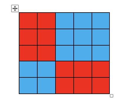
Figure 2.6: Illustration of global odds ratio.

• For cell \((i = 3, j = 2)\), the global odds ratio is defined as follows:
  • in the numerator is the product of the sums of the two groups of cells in red, while
  • in the denominator is the product of the sums of the two groups of cells in blue.

2.6.2.3 Local or Global Odds Ratios?

• Odds ratios \(r_{ij}^L\) and \(r_{ij}^G\) treat both classification variables in a symmetric way (\(r_{ij}^L\) locally and \(r_{ij}^G\) cumulatively).

• We can also just treat one classification variable cumulatively and the other locally.

• For example, we can treat the columns’ variable \(Y\) cumulatively and the row variable \(X\) locally. Then the odds ratio is \[\begin{equation} r_{ij}^{C_Y} = \frac{(\sum_{l \leq j} \pi_{il}) (\sum_{l > j} \pi_{i+1,l})}{(\sum_{l > j} \pi_{il}) (\sum_{l \leq j} \pi_{i+1,l})} \qquad i = 1,...,I-1 \quad j = 1,...,J-1 \end{equation}\]

• The cumulative odds ratio \(r_{ij}^{C_X}\) is defined analogously, and is cumulative with respect to the rows, being applied on successive columns \(j\) and \(j + 1\).

• Cumulative and global odds ratios make sense for ordinal classification variables. They are also meaningful for tables with one ordinal classification variable and one binary.

• The ordinality of the classification variables is required only whenever a classification variable is treated cumulatively. Thus, the local odds ratios are also appropriate for nominal variables.

2.6.2.4 Sample Odds Ratios

• Corresponding sample odds ratios are calculated analogously to previous odds ratios, with, for example, the sample local odds ratio being defined as \[\begin{equation} \hat{r}_{ij}^L = \frac{n_{ij} n_{i+1,j+1}}{n_{i+1,j} n_{i, j+1}} \qquad i = 1,...,I-1 \quad j = 1,...,J-1 \end{equation}\] and the sample global odds ratio being defined as \[\begin{equation} \hat{r}_{ij}^G = \frac{\bigl (\sum_{k \leq i} \sum_{l \leq j} n_{kl} \bigr) \bigl (\sum_{k > i} \sum_{l > j} n_{kl} \bigr)}{\bigl (\sum_{k \leq i} \sum_{l > j} n_{kl} \bigr) \bigl (\sum_{k > i} \sum_{l \leq j} n_{kl} \bigr)} \qquad i = 1,...,I-1 \quad j = 1,...,J-1 \end{equation}\]

• If the linear trend test provides evidence of association, sample odds ratios \(\hat{r}\) can be used to investigate the association further.

2.6.2.5 Example

We calculate the different types of sample odds ratios for cell \((2,2)\) of Table 2.15, with the odds ratios corresponding to the remaining cells presented in Tables 2.17 and 2.18 respectively.

\[\begin{eqnarray} \hat{r}_{22}^L & = & \frac{n_{22} n_{33}}{n_{32} n_{23}} = \frac{22 \times 55}{60 \times 18} = 1.12037 \\ \hat{r}_{22}^G & = & \frac{(47+25+36+22) \times 55}{(41+60) \times (12+18)} = 2.359... \end{eqnarray}\]

Table 2.17: Local Odds Ratios between successive row categories \(i\) and \(i+1\) and column categories \(j\) and \(j+1\), these being indicated in each case by the row and column names.

	Result: Success-Partial	Partial-Failure
Dose: High-Medium	1.149	1.705
Dose: Medium-Low	2.395	1.120

Table 2.18: Global Odds Ratios as defined in the text, with \((i,j)\) being denoted by the row and column names.

	Result: Success	Partial
Dose: High	2.557	2.755
Dose: Medium	3.023	2.360

2.6.2.6 Expected (under hypothesis) Odds Ratios

• The value of \(r_{ij}\) under a specific hypothesis \(\mathcal{H}_0\) can also be calculated, and given as \(r_{0,ij}\). In this case, we would utilise the corresponding expected frequencies \(E_{ij}\) from each cell \((i,j)\). For example, \(r_{0,ij}^L\) is given by: \[\begin{equation} r_{0,ij}^L = \frac{E_{ij} E_{i+1,j+1}}{E_{i+1,j} E_{i, j+1}} \qquad i = 1,...,I-1 \quad j = 1,...,J-1 \nonumber \end{equation}\]

• As we know, \(E_{ij}\) are often not known under \(H_0\) and thus need to be estimated by \(\hat{e}_{ij}\). In this case, the maximum likelihood estimate of \(r_{0,ij}\) under a specific hypothesis \(\mathcal{H}_0\) can be utilised: For example, the ML estimate of \(r_{0,ij}^L\) is given by: \[\begin{equation} \hat{r}_{0,ij}^L = \frac{\hat{E}_{ij} \hat{E}_{i+1,j+1}}{\hat{E}_{i+1,j} \hat{E}_{i, j+1}} \qquad i = 1,...,I-1 \quad j = 1,...,J-1 \nonumber \end{equation}\]

References

Covey, L. S., A. H. Glassman, and F. Stetner. 1990. “Depression and Depressive Symptoms in Smoking Cessation.” Comprehensive Psychiatry 31 (4): 350–54.

Haberman, S. J. 1973. “The Analysis of Residuals in Cross-Classified Tables.” Biometrics 29: 205–20.

Mantel, N. 1963. “Chi-Square Tests with One Degree of Freedom- Extensions of the Mantel-Haenszel Procedure.” Journal of the American Statistical Association 58: 690–700.

Yates, F. 1934. “Contingency Tables Involving Small Numbers and the Chi Square Test.” Journal of the Royal Statistical Society Supplement 1: 217–35.

---

14. \(2 \times 2\) tables were studied in Statistical Inference II, but we review them here as they are a good place to start!↩︎

15. In general, a \(+\) in place of an index denotes summation over this index.↩︎

16. Note that the notation \(r^{12}\) used here is slightly different to the convention for nominal odds ratios for \(I \times J\) tables used later on, where more care is required to clearly distinguish what categories the odds ratio is between.↩︎

17. Also called \(n_{ij}\) contingency table, 2-way contingency table, or classification table.↩︎

18. \((i,j)\) is short for \((X=i, Y=j)\).↩︎

19. For the avoidance of confusion, note that bold \(\boldsymbol{n}\) here represents the vector of counts in each compartment \((i,j)\), and \(n_{++}\) denotes total sample size.↩︎

20. One such scenario is considered in Q2-12.↩︎

21. The ideas of these two tests were covered in Statistical Inference II, but we shall go into more theoretical detail here.↩︎

22. Q2-5a involves showing that Equation (2.6) holds.↩︎

23. Q2-5b involves showing that Equation (2.7) holds.↩︎

24. It is important to be weary of the word independent here; if we reject \(\mathcal{H}_0\), even correctly, then this evidence of dependence (as the opposite of independence) is really only evidence of association. One variable may provide information that is relevant to/useful for predicting the other (unknown) variable, but they may not be dependent in the sense of directly depending on each other in the real-world. This is simply the correlation is not the same as causation argument. In a sense we could call this test a test for association, however, the word independence is so well-rooted in the textbooks that I will go along with this misnomer, but encourage you to make sure that you understand that we are really testing for association, despite the name.↩︎

25. Q2-6a involves showing this.↩︎

26. Compare this expression with that given by Equation (2.5).↩︎

27. Recall that \(\hat{E}_{ij}\) are estimated \(E_{ij}\)-values, because they are being estimated from the data.↩︎

28. This is an important point. If this was an analysis aimed at aiding us make important inferences (that is, if this weren’t just an example but an exercise in making inferences for actually going mushroom-picking), I should consult a Biologist, or mushroom expert, before making these kinds of decisions about which mushrooms are deemed most similar. Alternatively, if there is no other basis for combining categories, we may combine the smallest categories into a single category other (you may have encountered this rule previously). Incidentally, you should not use the analysis presented here as a basis for mushroom-picking - I will not be held responsible for any ill effects of anybody eating dodgy mushrooms!↩︎

29. By estimated \(E_{ij}\) values, I mean \(\hat{E}_{ij}\), because they are being estimated from the data.↩︎

30. Think about the relative difference in the effect of applying Yates’ continuity correction on the \(X_{ij}^2\) values for \(j =\) conical in table 2.6 compared to the other cap categories.↩︎

31. Yates’s correction has been criticised as perhaps being a little too much…↩︎

32. see Section 1.4.5.2↩︎

33. Q2-6b involves showing that Equation (2.13) holds.↩︎

34. It is convention to denote this statistic as \(G^2\) (rather than just \(G\)).↩︎

35. Q2-7 concerns showing that Approximation (2.15) holds through second-order Taylor expansion.↩︎

36. Some texts refer to these residuals simply as standardised residuals since they are the most common choice.↩︎

37. Note that this would be notated as r_{11}^{22} using the above more general odds ratio notation for an \(I \times J\) table.↩︎