Chapter 3 Multi-Way Contingency Tables

Multi-way contingency tables are very common in practice, derived by the presence of more than two cross-classification variables.

3.1 Description

3.1.1 Three-way Tables

• Consider an $I \times J \times K$ contingency table $(n_{ijk})$ for $i = 1,...,I$, $j = 1,...,J$ and $k = 1,...,K$, with classification variables $X$ (the rows), $Y$ (the columns) and $Z$ (the layers) respectively.

• A schematic of a generic $X \times Y \times Z$ contingency table of counts is shown in Figure 3.1.

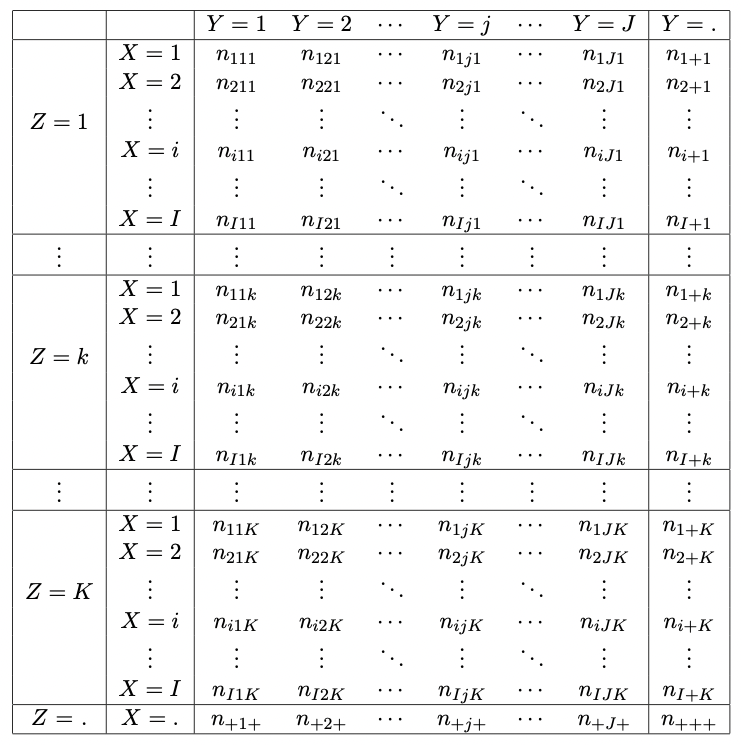
Figure 3.1: Generic I x J x K contingency table of counts.

• We can define the joint probability distribution of $(X,Y,Z)$ as $$\begin{equation} \pi_{ijk} = P(X=i, Y=j, Z=k) \end{equation}$$

• Proportions, observed and random counts are defined similarly to the $I \times J$ contingency table cases….

3.1.1.1 Example

The table in Figure 3.2 shows an example of a 3-way contingency table. This hypothetical data cross-classifies the response ($Y$) to a treatment drug ($X$) at one of two different clinics ($Z$).

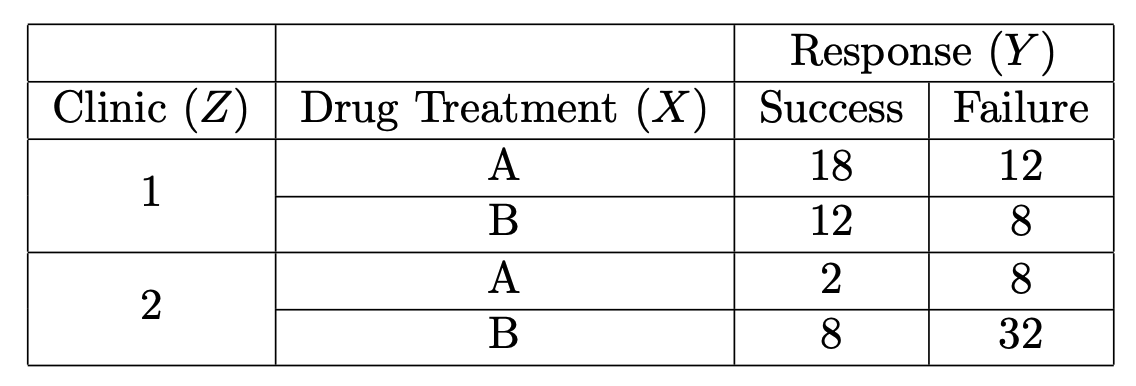
Figure 3.2: Table cross-classifying hypothetical treatment drug, response and clinic.

3.1.1.2 Partial/Conditional Tables

• Partial, or conditional, tables involve fixing the category of one of the variables.

• We denote the fixed variable in parentheses.

• For example, the set of $XY$-partial tables consist of the $K$ corresponding two-way layers, denoted as $(n_{ij(k)})$ for $k = 1,...,K$.

• $XZ$ and $YZ$- partial tables are denoted as $(n_{i(j)k})$ and $(n_{(i)jk})$ respectively.

• Partial/conditional probabilities: $$\begin{equation} \pi_{ij(k)} = \pi_{ij|k} = P(X=i, Y=j | Z=k) = \frac{\pi_{ijk}}{\pi_{++k}} \qquad k = 1,...,K \end{equation}$$

• Partial/conditional proportions: $$\begin{equation} p_{ij(k)} = p_{ij|k} = \frac{n_{ijk}}{n_{++k}} \qquad k = 1,...,K \end{equation}$$

3.1.1.3 Marginal Tables

• Marginal tables involve summing over all possible categories of a particular variable.

• We denote such summation using a $+$ (as before).

• For example, the $XY$- marginal table is $(n_{ij+}) = (\sum_k n_{ijk})$.

• $XZ$ and $YZ$- marginal tables are denoted as $(n_{i+k})$ and $(n_{+jk})$ respectively.

• Marginal probabilities: $$\begin{equation} \pi_{ij} = P(X=i, Y=j) = \pi_{ij+} = \sum_{k=1}^K \pi_{ijk} \end{equation}$$

• Marginal proportions: $$\begin{equation} p_{ij} = p_{ij+} = \sum_{k=1}^K p_{ijk} \end{equation}$$

3.1.1.4 Marginal Vectors

• Information on the single classification variables is summarised in the marginal vectors $(n_{1++},...,n_{I++})$, $(n_{+1+},...,n_{+J+})$ and $(n_{++1},...,n_{++K})$ respectively.

3.1.2 Generic Multiway Tables

• A multiway $I_1 \times I_2 \times ... \times I_q$ contingency table for variables $X_1,X_2,...,X_q$ will analogously be denoted as $(n_{i_1i_2...i_q})$, $i_l = 1,...,I_l$, $l = 1,...,q$.

• The definition of partial and marginal tables also follow analogously.

• For example, $(n_{i_1+(i_3)i_4(i_5)})$ denotes the two-way partial marginal table obtained by summing over all levels/categories $i_2$ of $X_2$ for a fixed level/category of (or conditioning on) variables $X_3=i_3$ and $X_5=i_5$.

3.2 Odds Ratios

• Conditional and marginal odds ratios can be defined for any two-way conditional or marginal probabilities table of a multi-way $I_1 \times I_2 \times ... \times I_q$ table with $I_l \geq 2$, $l = 1,...,q$.

• In this case, the conditional and marginal odds ratios are defined as odds ratios for two-way tables of size $I \times J$.

• Thus, as defined for general two-way tables in Sections 2.5 and 2.6.2, there will be a (not unique) minimal set of odds ratios of nominal, local, cumulative, or global type.

• For example, for an $I \times J \times K$ table, the $XY$ local odds ratios conditional on $Z$ are defined by $$\begin{equation} r_{ij(k)}^{L, XY} = \frac{\pi_{ijk}\pi_{i+1,j+1,k}}{\pi_{i+1,j,k}\pi_{i,j+1,k}} \qquad i = 1,...,I-1 \quad j = 1,...,J-1 \quad k = 1,...,K \end{equation}$$ and the $XY$-marginal local odds ratios are defined by $$\begin{equation} r_{ij}^{L, XY} = \frac{\pi_{ij+}\pi_{i+1,j+1,+}}{\pi_{i+1,j,+}\pi_{i,j+1,+}} \qquad i = 1,...,I-1 \quad j = 1,...,J-1 \end{equation}$$

• The conditional and marginal odds ratios of other types, like nominal, cumulative and global, are defined analogously.

3.3 Types of Independence

• Let $(n_{ijk})$ be an $I \times J \times K$ contingency table of observed frequencies with row, column and layer classification variables $X$, $Y$ and $Z$ respectively.

• We consider various types of independence that could exist among these three variables.

3.3.1 Mutual Independence

• $X$, $Y$ and $Z$ are mutually independent if and only if $$\begin{equation} \pi_{ijk} = \pi_{i++} \pi_{+j+} \pi_{++k} \qquad i = 1,...,I \quad j = 1,...,J \quad k = 1,...,K \tag{3.1} \end{equation}$$

• Such mutual independence can be symbolised as $[X,Y,Z]$.

3.3.1.1 Example

• Following the example of Section 3.1.1.1, mutual independence would mean that clinic, drug and response were independent of each other.

• In other words, knowledge of the values of one variable doesn’t affect the probabilities of the levels of the others.

3.3.2 Joint Independence

• If $Y$ is jointly independent from $X$ and $Z$ (without these two being necessarily independent), then $$\begin{equation} \pi_{ijk} = \pi_{+j+} \pi_{i+k} \qquad i = 1,...,I \quad j = 1,...,J \quad k = 1,...,K \tag{3.2} \end{equation}$$

• Such joint independence can be symbolised as $[Y,XZ]$.

• By symmetry, there are two more hypotheses of this type, which can be expressed in a symmetric way to Equation (3.2) for $X$ or $Z$ being jointly independent from the remaining two variables. These could be symbolised as $[X, YZ]$ and $[Z, XY]$ respectively.

3.3.2.1 Example

If $[Z,XY]$, then the clinic is independent of the drug and the response. In other words, the response of a subject to treatment may depend on the drug they received, but neither of these are associated with the clinic that they went to.

3.3.3 Marginal Independence

• $X$ and $Y$ are marginally independent (ignoring $Z$) if and only if $$\begin{equation} \pi_{ij+} = \pi_{i++} \pi_{+j+} \qquad i = 1,...,I \quad j = 1,...,J \quad k = 1,...,K \tag{3.3} \end{equation}$$

• Here, we actually ignore $Z$.

• Such marginal independence is symbolised $[X,Y]$.

3.3.3.1 Example

• If $Y$ and $Z$ are marginally independent³⁸ (that is $[Y,Z]$), then this would imply that response to treatment is not associated with the clinic attended if we ignore which drug was received.

3.3.4 Conditional Independence

• Under a multinomial sampling scheme, the joint probabilities of the three-way table cells $\pi_{ijk}$ can be expressed in terms of conditional probabilities as $$\begin{eqnarray} \pi_{ijk} & = & P(X=i, Y=j, Z=k) \\ & = & P(Y=j| X=i, Z=k) \, P(X=i, Z=k) \\ & = & \pi_{j|ik} \pi_{i+k} \end{eqnarray}$$

• $X$ and $Y$ are conditionally independent given $Z$ if $$\begin{equation} \pi_{ij|k} = \pi_{i|k} \pi_{j|k} \qquad k = 1,...,K \end{equation}$$

• We can consequently show that $$\begin{equation} \pi_{j|ik} = \pi_{j|k} \end{equation}$$ and therefore that $$\begin{eqnarray} \pi_{ijk} = \pi_{j|k} \pi_{i+k} & = & P(Y=j|Z=k) P(X=i,Z=k) \nonumber \\ & = & P(X=i,Z=k) \frac{P(Y=j,Z=k)}{P(Z=k)} \nonumber \\ & = & \frac{\pi_{i+k}\pi_{+jk}}{\pi_{++k}} \tag{3.4} \\ && \qquad \qquad i = 1,...,I \quad j = 1,...,J \quad k = 1,...,K \nonumber \end{eqnarray}$$

• Note that we here assumed that $Y$ was the response variable. The conditioning approach with $X=i$ as response variable would also lead to Equation (3.4), which is symmetric in terms of $X$ and $Y$.

• This conditional independence of $X$ and $Y$ given $Z$ can be symbolised as $[XZ,YZ]$.

• The hypotheses of conditional independence $[XY, YZ]$ and $[XY,XZ]$ are formed analogously to Equation (3.4).

3.3.4.1 Example

If $Y$ and $Z$ are conditionally independent given $X$ (that is, $[XY,XZ]$), this implies that response to treatment is independent of clinic attended given knowledge of which drug was received.

3.3.4.2 Odds Ratios

• Under conditional independence of $X$ and $Y$ given $Z$ ([XZ,YZ]), the $XZ$ odds ratios conditional on $Y$ are equal to the $XZ$ marginal odds ratios, that is³⁹ $$\begin{equation} r_{i(j)k}^{XZ} = r_{ik}^{XZ} \qquad i = 1,...,I-1 \quad j = 1,...,J \quad k = 1,...,K-1 \tag{3.5} \end{equation}$$ In other words, the marginal and conditional $XZ$ associations coincide.

• By symmetry, we also have that $$\begin{equation} r_{(i)jk}^{YZ} = r_{jk}^{YZ} \qquad i = 1,...,I \quad j = 1,...,J-1 \quad k = 1,...,K-1 \end{equation}$$ that is, the marginal and conditional $YZ$ associations coincide.

• However, the $XY$ marginal and conditional associations do not coincide, that is: $$\begin{equation} r_{ij(k)}^{XY} \neq r_{ij}^{XY} \end{equation}$$ in general.

• Such arguments for $[XY,YZ]$ and $[XY,XZ]$ are analogous.

3.3.5 Conditional and Marginal Independence

Important: Conditional independence does not imply marginal independence, and marginal independence does not imply conditional independence.

3.3.5.1 Example

3.3.5.1.1 Marginal but not Conditional Independence

• Suppose response $Y$ and clinic $Z$ are marginally independent (ignoring treatment drug $X$). However, there may be a conditional association between response to treatment $Y$ and clinic attended $Z$ on the drug received $X$.

• Example potential explanation⁴⁰: some clinics may be better prepared to care for subjects on some treatment drugs than others, but without knowledge of the treatment drug received, neither clinic is more associated with a successful response.

3.3.5.1.2 Conditional but not Marginal Independence

• Suppose $Y$ and $Z$ are conditionally independent given $X$ (that is, $[XY,XZ]$), then this implies that response to treatment is independent of clinic attended given knowledge of which drug was received. However, there may be a marginal association between response to treatment $Y$ and clinic attended $Z$ if we ignore which treatment drug $X$ was received.

• Example potential explanation: Given knowledge of the treatment drug, it does not matter which clinic the subject attends. However, without knowledge of the treatment drug, one clinic may be more associated with a successful response (perhaps because their stock of the more successful drug is greater…).

3.3.6 Homogeneous Associations

• Homogeneous associations (also known as no three-factor interactions) mean that the conditional relationship between any pair of variables given the third one is the same at each level of the third variable; but not necessarily independent.

• This relation implies that if we know all two-way tables between the three variables, we have sufficient information to compute $(\pi_{ijk})$.

• However, there are no separable closed-form estimates for the expected joint probabilities $(\hat{\pi}_{ijk})$, hence maximum likelihood estimates must be computed by an iterative procedure such as Iterative Proportional Fitting or Newton-Raphson.

• Such homogeneous associations are symbolised $[XY, XZ, YZ]$.

3.3.6.1 Odds Ratios

• Homogeneous associations can be thought of in terms of conditional odds ratios as follows:

  • the $XY$ partial odds ratios at each level of $Z$ are identical: $r_{ij(k)}^{XY} = r_{ij}^{XY, \star}$

  • the $XZ$ partial odds ratios at each level of $Y$ are identical: $r_{i(j)k}^{XZ} = r_{ik}^{XZ, \star}$

  • the $YZ$ partial odds ratios at each level of $X$ are identical: $r_{(i)jk}^{YZ} = r_{jk}^{YZ, \star}$

• Note that $r_{ij}^{XY, \star}, r_{ik}^{XZ, \star}, r_{jk}^{YZ, \star}$ are not necessarily the same as the corresponding marginal odds ratios $r_{ij}^{XY}, r_{ik}^{XZ}, r_{jk}^{YZ}$.

3.3.6.2 Example

The treatment response and treatment drug have the same association for each clinic.

More precisely, we have $$\begin{equation} r_{A,S,(k)}^{XY} = r_{A,S}^{XY, \star} \iff \frac{\pi_{A,S,(k)}}{ \pi_{A,F,(k)}} = r_{A,S}^{XY, \star} \frac{\pi_{B,S,(k)}}{\pi_{B,F,(k)}} \qquad k = 1,2 \end{equation}$$ which means that each drug has a different odds of success depending on the clinic, however, the odds of treatment success of drug $A$ are a fixed constant $r_{A,S}^{XY, \star}$ greater than the odds of treatment success of drug $B$, regardless of the clinic.

3.3.7 Tests for Independence

• Marginal independence (Equation (3.3)) can be tested using the test for independence presented in Section 2.4.3.1 applied on the corresponding two-way marginal table.

• Hypotheses of the independence statements defined by Equations (3.1), (3.2) and (3.4) could be tested analogously using the relevant marginal counts.

• We do not consider these tests, but defer to log-linear models (soon!).

• A specific test of independence of $XY$ at each level of $Z$ for $2 \times 2 \times K$ tables is presented in Section 3.3.10.

3.3.8 Summary of Relationships

We present a summary of which independence relationships can be implied from which others, and which can’t, in Figure 3.3.

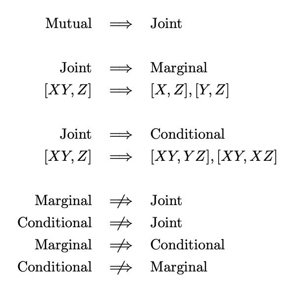
Figure 3.3: Summary of relationships between independencies.

3.3.9 Multi-way Tables

• Analogous definitions of the various types of independence exist for general multi-way tables.

3.3.9.1 Example

We might analyse $(n_{i_1+(i_3)i_4(i_5)})$ across the different levels of $(I_3,I_5)$ to see if $(I_1,I_4)$ and $(I_3,I_5)$ are marginally independent (ignoring $I_2$). We will explore this a bit, but in general, we look to log-linear models.

3.3.10 Mantel-Haenszel Test for $2 \times 2 \times K$ Tables

• We will discuss the particular case of $X$ and $Y$ being binary variables that are cross-classified across the $K$ layers of a variable $Z$, forming $K$ $2 \times 2$ partial tables $n_{ij(k)}, \, k = 1,...,K$.

• The Mantel-Haenszel Test is for testing the conditional independence of $X$ and $Y$ given $Z$ for these $2 \times 2 \times K$ tables, that is, it considers the hypotheses $$\begin{eqnarray} \mathcal{H}_0: & \, X,Y \textrm{are independent conditional on the level of } Z. \\ \mathcal{H}_1: & \, X,Y \textrm{are not independent conditional on the level of } Z. \end{eqnarray}$$ or in other words⁴¹ $$\begin{eqnarray} \mathcal{H}_0: & \, r_{12(k)} = 1, \, \textrm{for all} \, k = 1,...,K \\ \mathcal{H}_1: & \, r_{12(k)} \neq 1, \, \textrm{for some} \, k = 1,...,K \\ \end{eqnarray}$$

• The Mantel-Haenszel Test conditions on the row and column marginals of each of the $K$ partial tables.

• Under $\mathcal{H}_0$, every partial table has that $n_{11k}$ follows a hypergeometric distribution⁴² $\mathcal{H} g(N = n_{++k}, M = n_{1,+,k}, q = n_{+,1,k})$⁴³, and thus has mean and variance $$\begin{equation} \hat{E}_{11k} = \frac{n_{1+k} n_{+1k}}{n_{++k}} \qquad \qquad \hat{\sigma}^2_{11k} = \frac{n_{1+k} n_{2+k} n_{+1k} n_{+2k}}{n^2_{++k}(n_{++k} - 1)} \nonumber \end{equation}$$

• $\sum_k n_{11k}$ therefore has mean $\sum_k \hat{E}_{11k}$ and variance $\sum_k \hat{\sigma}^2_{11k}$, since the values of $n_{11k}$ are independent of each other (having conditioned on $Z=k$).

• The Mantel–Haenszel test statistic is defined as⁴⁴ $$\begin{equation} T_{MH} = \frac{[\sum_k (n_{11k} - \hat{E}_{11k})]^2}{\sum_k \hat{\sigma}_{11k}^2} \tag{3.6} \end{equation}$$

• $T_{MH}$ is asymptotically $\chi^2_1$ under $\mathcal{H}_0$.

• If $T_{MH(obs)}$ is the observed value of the test statistic for a particular case, then the $p$-value is $P(\chi_1^2 > T_{MH(obs)})$.

• When the $XY$ association is similar across the partial tables, then the test is more powerful.

• It loses in power when the underlying associations vary across the layers, especially when they are of different direction, since the differences $n_{11k} - \hat{E}_{11k}$ will then cancel out in the sum of the statistic given by Equation (3.6).

---

38. ignoring $X$↩︎

39. Note that we don’t superscript $L$ or $G$ here, as the result holds for both. Q3-2 involves showing that Equation (3.5) holds for local odds ratios.↩︎

40. Note that this is precisely what this is - a potential explanation - it would be incorrect to conclude that this is definitely the reason for the hypothesised independence scenarios. We all know (I hope…) that (or in this case, ) .↩︎

41. Note that we revert back to the $r_{12}$ notation here since each of the $K$ layers is a $2 \times 2$ table.↩︎

42. See Section 1.4.4.↩︎

43. Why hypergeometric? Well, for any $2 \times 2$ table we have an assumed total of $N = n_{++k}$ items. We condition on row and column margins, so we assume knowledge of $n_{i,+,k}$ and $n_{+,j,k}$. In that population, we know that $M= n_{1,+,k}$ of these items are such that $i=1$. If the two variables $X$ and $Y$ are conditionally independent given $Z$, then we could view $N_{1,1,k}$ to be the result of picking $q = n_{+,1,k}$ items (those going into column 1) randomly from $N = n_{++k}$, and calculating how many of those are from row 1 (given that we know that there are $M=n_{1,+,k}$ items out of the $N$ that will go into row 1 in total). Therefore $N_{1,1,k} \sim \mathcal{H} g(N = n_{++k}, M = n_{1,+,k}, q = n_{+,1,k})$↩︎

44. Note that the square is outside of the summation.↩︎