Chapter 10 Problems
Chapter 1
Q1-1: Introductory Questions
- What is a model?
- What is a statistical model?
- What is an advanced statistical model?
- What is a variable?
- What is a random variable?
Q1-2: Types of Variable
Decide whether the following variables are categorical or numerical, and classify further if possible:
gender of the next lamb born at the local farm.
number of times a dice needs to be thrown until the first \(6\) is observed.
amount of fluid (in ounces) dispensed by a machine used to fill bottles with lemonade.
thickness of penny coins in millimetres.
assignment grades of a 3H Mathematics course (from A to D).
marital status of some random sample of citizens.
Q1-3: Properties of Probability Distributions
Prove the results for the expectation and covariance structure of the multinomial distribution stated in Section 1.4.3.1.
Suppose \(X_1^2,...,X_m^2\) are \(m\) independent variables with chi-squared distributions \(X_i^2 \sim \chi^2(n_i)\). Show that \[\begin{equation} \sum_{i=1}^m X_i^2 = \chi^2(\sum_{i=1}^m n_i ) \end{equation}\]
Suppose \(X^2\) has the distribution \(\chi^2(n)\). Prove that \[\begin{align} {\mathrm E}[X^2] & = n \\ {\mathrm{Var}}[X^2] & = 2n \end{align}\] Hint: Your solution may require you to assume or show that \({\mathrm E}[Z^4] = 3\), where \(Z \sim{\mathcal N}(0,1)\).
Chapter 2
Q2-1: Quickfire Questions
- What is the difference between a Poisson, Multinomial and product Multinomial sampling scheme?
- What does an odds of 1.8 mean relative to success probability \(\pi\)?
Q2-2: Sampling Schemes
Write down statements for the expectation and variance of a variable following a product Multinomial sampling scheme as described in Section 2.3.3.
Q2-3: Fatality of Road Traffic Accidents
Table 10.1 shows fatality results for drivers and passengers in road traffic accidents in Florida in 2015, according to whether the person was wearing a shoulder and lap belt restraint versus not using one. Find and interpret the odds ratio.
| Injury: Fatal | Non-Fatal | Sum | |
|---|---|---|---|
| Restraint Use: No | 433 | 8049 | 8482 |
| Restraint Use: Yes | 570 | 554883 | 555453 |
| Sum | 1003 | 562932 | 563935 |
Q2-4: Difference of Proportions or Odds Ratios?
A 20-year study of British male physicians (Doll and Peto (1976)) noted that the proportion who died from lung cancer was 0.00140 per year for cigarette smokers and 0.00010 per year for non-smokers. The proportion who died from heart disease was 0.00669 for smokers and 0.00413 for non-smokers.
Describe and compare the association of smoking with lung cancer and with heart disease using the difference of proportions.
Describe and compare the association of smoking with lung cancer and heart disease using the odds ratio.
Which response (lung cancer or heart disease) is more strongly related to cigarette smoking, in terms of increased proportional risk to the individual?
Which response (lung cancer or heart disease) is more strongly related to cigarette smoking, in terms of the reduction in deaths that could occur with an absence of smoking?
Q2-6: Maximum Likelihood by Lagrange Multipliers
- Consider a Multinomial sampling scheme, and that \(X\) and \(Y\) are independent. We need to find the MLE of \(\boldsymbol{\pi}\), but now we have that \[\begin{equation} \pi_{ij} = \pi_{i+} \pi_{+j} \end{equation}\] The log likelihood is \[\begin{eqnarray} l(\boldsymbol{\pi}) & \propto & \sum_{i,j} n_{ij} \log (\pi_{ij}) \\ & = & \sum_{i} n_{i+} \log (\pi_{i+}) + \sum_{j} n_{+j} \log (\pi_{+j}) \end{eqnarray}\] Use the method of Lagrange multipliers to show that \[\begin{eqnarray} \hat{\pi}_{i+} & = & \frac{n_{i+}}{n_{++}} \\ \hat{\pi}_{+j} & = & \frac{n_{+j}}{n_{++}} \end{eqnarray}\]
Hint: You may wish to go through the following steps to achieve this:
- Write down the constraints.
- Write down the Lagrange function.
- State the equations satisfied at the local optima.
- Rearrange for \(\hat{\lambda}_1, \hat{\lambda}_2\) and thus \(\hat{\pi}_{i+}\) and \(\hat{\pi}_{+j}\).
Q2-7: Second-Order Taylor Expansion
Show that Approximation (2.15) of Section 2.4.5.1 holds.
Hint: Equation (2.15) can be shown by first letting \(n_{ij} = \hat{E}_{ij} + \delta_{ij}\), where \(\sum_{ij} \delta_{ij} = 0\), and then considering a second-order Taylor expansion of \(\log(1 + \frac{\delta_{ij}}{\hat{E}_{ij}})\) around \(1\) .
Q2-8: Relative Risk
In 1998, A British study reported that “Female smokers were 1.7 times more vulnerable than Male smokers to get lung cancer.” We don’t investigate whether this is true or not, but is 1.7 the odds ratio or the relative risk? Briefly (one sentence maximum) explain your answer.
A National Cancer institute study about tamoxifen and breast cancer reported that the women taking the drug were \(45\%\) less likely to experience invasive breast cancer than were women taking a placebo. Find the relative risk for (i) those taking the drug compared with those taking the placebo, and (ii) those taking the placebo compared with those taking the drug.
Q2-9: The Titanic
For adults who sailed on the Titanic on its fateful voyage, the odds ratio between gender (categorised as Female or Male), and survival (categorised as yes or no) was 11.4 (Dawson (1995)).
It is claimed that “The Probability of survival for women was 11.4 times that for men”. i) What is wrong with this interpretation? ii) What should the correct interpretation be? iii) When would the quoted interpretation be approximately correct?
The odds of survival for women was 2.9. Find the proportion of each gender who survived.
Q2-10: Test and Reality
For a diagnostic test of a certain disease, let \(\pi_1\) denote the probability that the diagnosis is positive given that a subject has the disease, and let \(\pi_2\) denote the probability that the diagnosis is positive given that a subject does not have the disease. Let \(\tau\) denote the probability that a subject has the disease.
More relevant to a patient who has received a positive diagnosis is the probability that they truly have the disease. Given that a diagnosis is positive, show that the probability that a subject has the disease (called the positive predictive value) is \[\begin{equation} \frac{\pi_1 \tau}{\pi_1 \tau + \pi_2 (1-\tau)} \end{equation}\]
Suppose that a diagnostic test for a disease has both sensitivity and specificity equal to 0.95, and that \(\tau = 0.005\). Find the probability that a subject truly has the disease given a positive diagnostic test result.
Create a \(2 \times 2\) contingency table of cross-classified probabilities for presence or absence of the disease and positive or negative diagnostic test result.
Calculate the odds ratio and interpret.
Q2-11: Happiness and Income
Table 10.2 shows data from a General Social Survey cross-classifying a person’s perceived happiness with their family income.
Perform a \(\chi^2\) test of independence between the two variables.
Calculate and interpret the adjusted residuals for the four corner cells of the table.
| Happiness: Not too Happy | Pretty Happy | Very Happy | |
|---|---|---|---|
| Income: Above Average | 21 | 159 | 110 |
| Income: Average | 53 | 372 | 221 |
| Income: Below Average | 94 | 249 | 83 |
Q2-12: Tea! (Fisher’s Exact Test of Independence)
This is a quote from Fisher (1937)74:
A lady declares that by tasting a cup of tea made with milk she can discriminate whether the milk or the tea infusion was first added to the cup. We will consider the problem of designing an experiment by means of which this assertion can be tested. For this purpose let us first lay down a simple form of experiment with a view to studying its limitations and its characteristics, both those which appear to be essential to the experimental method, when well developed, and those which are not essential but auxiliary.
Our experiment consists in mixing eight cups of tea, four in one way and four in the other, and presenting them to the subject for judgement in a random order. The subject has been told in advance of what the test will consist, namely that she will be asked to taste eight cups, that these shall be four of each kind, and that they shall be presented to her in a random order, that is in an order not determined arbitrarily by human choice, but by the actual manipulation of the physical apparatus used in games of chance, cards, dice, roulettes, etc., or more expeditiously, from a published collection of random sampling numbers purporting to give the actual results of such manipulation. Her task is to divide the 8 cups into two sets of 4, agreeing, if possible, with the treatments received.
From the text, we know that there are 4 cups with milk added first and 4 with tea infusion added first. How many distinct orderings can these 8 cups to be tasted take, in terms of type.
Note that the lady also knows that there are four cups of each type, and must group them into two sets of four (those she thinks had milk added first, and those she thinks had tea infusion added first). Given that the lady guesses milk first three times when indeed the milk was added first, cross-classify the lady’s guesses against the truth in a \(2 \times 2\) contingency table.
Fisher presented an exact75 solution for testing the null hypothesis \[\begin{equation} \mathcal{H}_0: r_{12} = 1 \end{equation}\] against the one-sided alternative \[\begin{equation} \mathcal{H}_1: r_{12} > 1 \end{equation}\] for contingency tables with fixed row and column sums.
What hypothesis does \(\mathcal{H}_0\) correspond to in the context of the tea tasting test described above? Write down an expression for \(P(N_{11} = t)\) under \(\mathcal{H}_0\). Thus, perform a (Fisher’s exact76) hypothesis test to test the lady’s claim that she can indeed discriminate whether the milk or tea infusion was first added to the cup.Suppose the lady had correctly classified all eight cups as having either milk or tea infusion added first. Would Fisher’s exact hypothesis test provide evidence of her ability now?
Q2-13: US Presidential Elections
Table 10.3 cross-classifies a sample of votes in the 2008 and 2012 US Presidential elections. Test the null hypothesis that vote in 2008 was independent from vote in 2012 by estimating, and finding a \(95\%\) confidence interval for, the population odds ratio.
| Vote 2012: Obama | Romney | |
|---|---|---|
| Vote 2008: Obama | 802 | 53 |
| Vote 2008: McCain | 34 | 494 |
Q2-14: Job Security and Happiness
Consider the table presented in Figure 10.1 summarising the responses for extent of agreement to the statement “job security is good” (JobSecOK, or Job Security) and general happiness (Happiness) from the 2018 US General Social Surveys. Additional possible responses of don’t know and no answer are omitted here.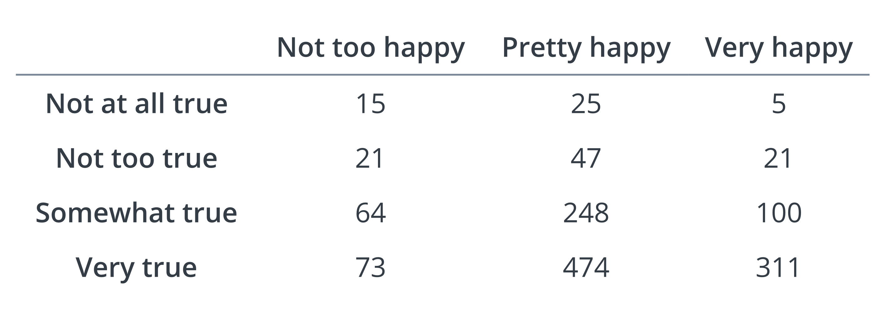
Figure 10.1: Contingency Table for Q2-14
Calculate a minimal set of local odds ratios. Interpret and discuss.
Calculate a minimal set of odds ratios, treating job security locally and happiness cumulatively. Interpret and discuss.
Calculate a minimal set of odds ratios, treating job security as a nominal variable (taking very true as the reference category) and happiness as a cumulative variable. Interpret and discuss.
Calculate a minimal set of global odds ratios, that is, treating both job security and happiness as cumulative variables.
Calculate a \(95\%\) confidence interval for the global odds ratio, with the first two categories of each variable being grouped together into one category in each case.
Perform a linear trend test to assess whether there is any evidence of association between Happiness and Job Security.
Q2-15: A New Treatment?
A study investigates the relationship between a new treatment (Treatment A) and a standard treatment (Treatment B) for reducing symptoms of a specific disease. Patients are classified as either having symptoms reduced (Yes) or not reduced (No). The data from the study are as shown in Figure 10.2.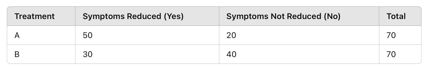
Figure 10.2: Contingency Table for Q2-15
Calculate the odds ratio of symptoms being reduced for patients receiving Treatment A compared to those receiving Treatment B. Interpret.
Using the data provided, apply a generalized likelihood ratio test to determine if there is a significant association between treatment type and symptom reduction at the \(5\%\) significance level.
Chapter 3
Q3-1: A Question of Notation
- Based on the notation of Section 3.1, state what table (in terms of dimension, as well as conditioning and marginalising of variables) is being described by:
\((n_{(i)jk})\)
\((n_{(i)+k(l)})\)
\((n_{i_1i_2+(i_4)i_5(i_6)+})\)
Use the notation of Section 3.1, in the context of Section 3.1.1.1, to notate and construct the conditional (on drug treatment \(X = B\)) table, having marginalised over clinic \(Z\).
Assuming a total of 8 variables, use the notation of Section 3.1 to notate the partial marginal table obtained by summing over all levels of variables \(i_3, i_5\) and \(i_7\), for a fixed level of variables \(i_1\) and \(i_4\).
Q3-2: Conditional and Marginal Local Odds Ratios
Show that Equation (3.5) of Section 3.3.4.2 holds for local odds ratios under the conditional independence of \(X\) and \(Y\) given \(Z\). Recall that such conditional independence means that Equation (3.4) holds.
Q3-3: Types of Independence
In Section 3.3, we discussed different types of independence, such as mutual, joint, marginal and conditional, as well as homogeneous associations. Throughout, I illustrated what the different independence assumptions might mean in the context of the three variables Drug Treatment (\(X\)), Response (\(Y\)) and Clinic (\(Z\)) of the example introduced in Section 3.1.1.1.
Think of another example with three (or more…) categorical variables (with at least two levels each), and consider what the different types of independence would imply about the associations (or lack thereof) between the three variables. Note that I am not interested in any numbers here - it is about the implications of any hypothesised independence scenario - so all we need are three variable names with possible categories. You may wish to use a hypothetical example of your own construction, or one that you have found from other sources.
You may wish to hypothesise possible reasoning for each situation, such as I did in Section 3.3.5 with the . Note that the purpose of this is to get you thinking (like an expert might) of possible explanations in real-life scenarios that would lead to the various hypotheses about independence. It does not mean that strong evidence of any particular scenario of association necessarily implies that the explanation or reasoning is correct77.
You should discuss your answers to this question with your fellow students, and you are also welcome to discuss your answer with me during the weekly office hour.
I am well aware that many will be tempted to skip this question, but being able to convey the ideas reflected in our models or tests into practical examples is a very important part of being a Statistician (are we really doing Statistics at all if we don’t have this skill?). Even if this holistic reasoning does not motivate you, this skill will be tested in the end-of-year exam, and is often the source of lost marks among our students.
Q3-4: Conditional and Joint Independence
Consider an \(I \times J \times K\) contingency table, with classification variables \(X, Y, Z\). By writing down the relevant probability forms involved, or otherwise…
- Prove that if
- \(X\) and \(Y\) are conditionally independent given \(Z\); and
- \(X\) and \(Z\) are conditionally independent given \(Y\),
then \(Y\) and \(Z\) are jointly independent from \(X\).
- Prove that if \(Y\) and \(Z\) are jointly independent from \(X\), then
- \(X\) and \(Y\) are conditionally independent given \(Z\); and
- \(X\) and \(Z\) are conditionally independent given \(Y\).
Q3-5: 1988 General Social Survey
The 1988 General Social Survey compiled by the National Opinion Research Center asked:
- “Do you support or oppose the following measures to deal with AIDS? (1) Have the government pay all of the health care costs of AIDS patients; (2) Develop a government information program to promote safe sex practices, such as the use of condoms.”
The table in Figure 10.3 summarizes opinions about health care costs (H) and the information program (I), classified also by the respondent’s gender (G).
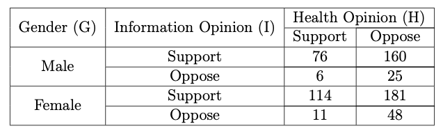
Figure 10.3: Source: 1988 General Social Survey, National Opinion Research Center.
Compute the marginal \(GH\)-table.
For the marginal \(GH\)-table, compute the MLE of the marginal odds ratio, along with a \(95\%\) confidence interval. Interpret the result.
Perform a Mantel Haenszel Chi-Square test, at the \(5\%\) level of significance, in order to test if the Information Opinion and the Health Opinion are independent at each level of Gender.
Compute the partial (conditional) \(IH\) odds ratio at each level of Gender. Interpret the result.
Q3-6: Alien Spacejets
The aliens are designing spacejets to enable them to travel between two planets. In particular, they need spacejets that can withstand the atmospheric pressure encountered whilst travelling through space between the two planets. They therefore cross-classify the survival of different spacejets on test runs in the atmosphere (Survives, \(Y\): yes or no) against Type, \(Z\): \(A\) or \(B\) and Colour, \(X\): red or green. The dataset is presented in the table shown in Figure 10.4.
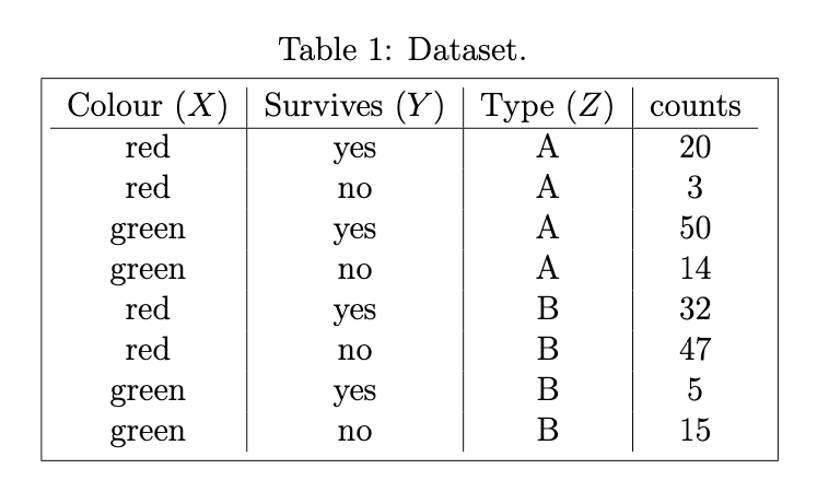
Figure 10.4: Table of Data for Q3-6.
Calculate the marginal \(XY\) contingency table of the observed counts.
Calculate an estimate of, along with a \(90\%\) confidence interval for, the marginal odds ratio of Colour and Survives.
What does the estimated odds ratio tell us about the relation between Colour and Survives? Infer whether there is evidence that Colour and Survives are dependent or not.
Based on the results of Parts (a)-(c), the aliens are convinced that the dataset provides at least some evidence that, regardless of Type, green spacejets have a greater chance of surviving the intense atmospheric pressure than red spacejets. Perform reasonable analyses to:
- illustrate to the aliens why they have jumped to the wrong conclusion, and
- discuss alternative inferences.
Supposing this was an excerpt from an exam question (as it may have been in the past), credit would be awarded for the clarity of your answer.
Q3-7 The Aliens in Durham
Suppose a horde of 216 aliens (beings from a far-off planet) arrive in Durham and are surveyed about the suitability of building structures were they to make Durham their home (they need to report back to the rest of their species). Suppose the rest of their kind is interested in knowing whether the opinion about suitability is associated with alien height (short, average-height, tall) and alien type (A,B). They therefore cross-classify these variables in the contingency table presented in Figure 10.5.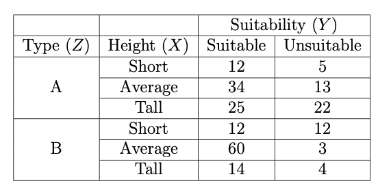
Figure 10.5: Contingency Table of Data for Q3-7.
Calculate an estimate of, along with a \(95\%\) confidence interval for, the marginal odds ratio of Suitability and Type.
Calculate a minimal set of marginal (over Type) global odds ratios between Height and Suitability, along with a reasonable \(95\%\) confidence interval for each. What assumption about variable Height is being made in order to do this? Interpret and explain the results in terms of associations between Height and Suitability.
Chapter 4
Q4-2: Two-way Mutual Independence Model
Assume a LLM with dependency structure \([X,Y]\) under a Poisson sampling scheme with corner point constraints.
Write down the appropriate LLM expression corresponding to dependency structure \([X,Y]\).
Rearrange the appropriate LLM expression for the corresponding \(\lambda\) parameters.
Write down the log-likelihood equations, and hence use the method of Lagrange multipliers to show that \[\begin{eqnarray} \hat{E}_{++} = E_{++}(\hat{\boldsymbol{\lambda}}) & = & n_{++} \nonumber \\ \hat{E}_{i+} = E_{i+}(\hat{\boldsymbol{\lambda}}) & = & n_{i+} \qquad i = 1,...,I \nonumber \\ \hat{E}_{+j} = E_{+j}(\hat{\boldsymbol{\lambda}}) & = & n_{+j} \qquad j = 1,...,J \nonumber \end{eqnarray}\]
Using the results of parts (b) and (c), or otherwise, find the MLEs of the LLM \(\lambda\) coefficients.
Q4-3: Hierarchical Log Linear Models
Identify if the following models are hierarchical, and for the ones that are, use the square bracket \([]\) notation (e.g. \([X,Y]\) for the two-way independence model) presented throughout Sections 3 and 4 to represent them, and discuss what assumptions about the associations between the variables they convey: \[\begin{eqnarray} \textrm{i. } \log E_{ijk} & = & \lambda + \lambda_i^X + \lambda_j^Y + \lambda_k^Z + \lambda_{jk}^{YZ} \qquad \forall i,j,k \nonumber \\ \textrm{ii. } \log E_{ijkl} & = & \lambda + \lambda_i^X + \lambda_j^Y + \lambda_k^Z + \lambda_l^W + \lambda_{ij}^{XY} + \lambda_{il}^{XW} + \lambda_{kl}^{ZW} + \lambda_{ikl}^{XZW} \qquad \forall i,j,k,l \nonumber \\ \textrm{iii. }\log E_{ijkl} & = & \lambda + \lambda_i^X + \lambda_j^Y + \lambda_k^Z + \lambda_l^W + \lambda_{ik}^{XZ} + \lambda_{il}^{XW} + \lambda_{kl}^{ZW} + \lambda_{ikl}^{XZW} \qquad \forall i,j,k,l \nonumber \end{eqnarray}\]
Write down the hierarchical log-linear models corresponding to
\([XY, XZ]\)
\([XY, XZ, XW]\)
\([X_1X_3, X_2X_3X_4, X_4X_5, X_5X_6]\)
and discuss what assumptions about the associations between the variables they convey.
- For the model discussed in part b-iii above, are variables \(X_1\) and \(X_6\) necessarily independent? Explain your answer.
Q4-5: \(2 \times 2 \times 2\) Contingency Table
Consider a \(2 \times 2 \times 2\) Contingency Table with classification variables \(X\), \(Y\) and \(Z\).
State the equation of the Log-linear model describing the dependency type \([XY,XZ]\).
Apply the two types of the non-identifiability constraints (corner points and sum-to-zero).
Write down the number of free parameters, and explain how you calculated them.
For parts (d) and (e), consider the corner point constraints only.
Express \(\log(\pi_{1|jk} / \pi_{2|jk})\) as a function of the linear model \(\lambda\) coefficients.
Express \(\log(r^{XY}_{ij(k)})\), that is, the log conditional (on \(Z\)) odds ratio, as a function of the linear model \(\lambda\) coefficients. Give a short interpretation of \(\lambda_{11}^{XY}\) based on this.
Q4-6: Exam-Style Question
All possible hierarchical log-linear models were fitted to a contingency table, based on a sample of 312 individuals, for three factors: X (2 levels), Y (3 levels) and Z (5 levels). The sampling scheme that was implemented was the Poisson sampling scheme. The results are shown in the table in Figure 10.6.
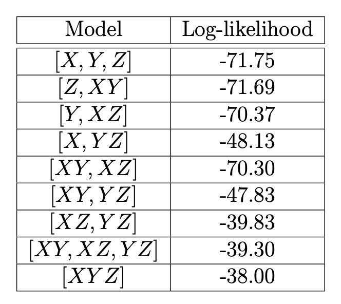
Figure 10.6: Table for Q4-5.
Calculate the number of free parameters resulting after applying corner point non-identifiability constraints for each model in the table.
Define the Akaike Information Criterion (AIC) and Bayes Information Criterion (BIC), then compute both AIC and BIC for each model in the table.
Identify which model is selected by each criterion and give a short explanation of what each criterion is intended to achieve.
Explain precisely what model \([XY,YZ]\) says about the dependence of factor \(Y\) on the other two factors.
Chapter 5
Q5-1: Tokyo Rainfall
We consider rainfall data recorded in Tokyo in the first 11 days of the year 1983, as given by the table in Figure 10.7. For each day, we know whether it rained (\(z_i=1\)) or did not rain (\(z_i=0\)) on that day: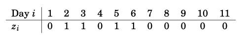
Figure 10.7: Rainfall data in Tokyo in the first 11 days of the year 1983.
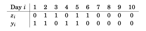
Figure 10.8: Rainfall data in Tokyo for the first 10 days of the year 1983 along with data about whether it rained the following day.
Formulate a logistic regression model for \(\pi(z)\) (consider the elements stated in Section 5.3.2), using the linear predictor \(\eta=\beta_{1}+\beta_{2} z\), that is, take the predictors to be \(x_{1} \equiv 1\) and \(x_{2} = z\).
Formulate the score function \(S(\boldsymbol{\beta})\).
Solve the estimating equation \(S(\hat{\boldsymbol{\beta}})=0\).
According to BBC Weather, it didn’t rain in Tokyo on Thursday November 17, 2022. Use your model to predict the rainfall probability in Tokyo on Friday November 18, 2022.
Chapter 6
Q6-1: Properties of the Exponential Dispersion Family
Let the distribution for \(Y\) be an exponential dispersion family: \[\begin{equation} P_{}\left(y |\theta(\mu), \phi\right) = \exp \bigl[ \frac{y\theta(\mu) - b(\theta(\mu))}{ \phi} + c(y, \phi) \bigr] \end{equation}\]
where \(\mu(\theta) = {\mathrm E}[Y |\theta, \phi]\).
Use the fact that \(\mu(\theta)\) and \(\theta(\mu)\) are inverses to show that \(\theta'(\mu) = 1/\mathcal{V}(\mu)\), where \(\mathcal{V}(\mu)\) is the variance function.
Show that with one data point \((\boldsymbol{x}, y)\), the maximum likelihood estimator for \(\mu\) is \(y\).
Chapter 7
Q7-1: The Gamma Distribution
We consider the exponential dispersion family (EDF)
\[\begin{equation} P(y | \theta, \phi) = \exp\{\frac{y \theta- b(\theta)}{\phi} + c(y, \phi) \} \qquad y>0 \end{equation}\]
Show that the expectation of a distribution belonging to a EDF is given by \(b^{\prime}(\theta)\).
Show that the Gamma distribution with density \[\begin{equation} P(y | \nu, \alpha ) = \frac{\alpha^{\nu}}{\Gamma(\nu)}y^{\nu -1} e^{-\alpha y} \end{equation}\] (with shape parameter \(\nu\) and rate parameter \(\alpha\)) is a member of the EDF.
Note: The Gamma-function is defined by \(\Gamma(\nu)=\int_0^{\infty}e^{-t}t^{\nu-1}\, dt\quad (\nu >0)\).
Exploiting properties of the EDF, find the mean \(\mu\) and the variance of the Gamma distribution.
Reparametrize the density function so that it depends on the parameters \(\nu\) and \(\mu\).
For gamma-distributed response, identify the natural link for use in a generalized linear model. Why is this link function often unsuitable in practice? Suggest an alternative link function.
Q7-2: Coronary Heart Disease
We are given data collected in the framework of a study of coronary heart disease in the table presented in Figure 10.9. It shows 1329 patients cross-classified by the level of their serum cholesterol (below or above 260) and the presence or absence of heart disease.
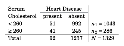
Figure 10.9: Table of data cross-classifying cholesterol (treated as a binary covariate) and presence or absence of heart disease.
We can consider this as a data set which is grouped with respect to a binary covariate, with values (say) \(z_1 = 0\) (if \(<260\)) and \(z_2 = 1\) (if \(\geq 260\)), and response defined through group-wise heart disease presence rates, that is \(y_1 = 51/1043\) and \(y_2 = 41/286\). We model this data through a Binomial logit model, that is \[\begin{equation} \pi(z_i) = \frac{\exp(\beta_1 + \beta_2 z_i)}{1 + \exp(\beta_1 + \beta_2 z_i)} \end{equation}\] where \(y_i|z_i \sim B(n_i, \pi(z_i)) / n_i\) (rescaled Binomial distribution).
Verify through differentiation of the log-likelihood that the score-function is given by \[\begin{equation} S(\beta_1, \beta_2) = \sum_{i=1}^2 n_i \Bigl( \begin{array}{c}1 \\ z_i \end{array} \Bigr) \bigl( y_i-\frac{\exp(\beta_1+ \beta_2z_i)}{1+ \exp(\beta_1+\beta_2 z_i)} \bigr) \end{equation}\]
Solve the score equation by hand (i.e. without R).
Comment on the relationship between this and the solution to Q5-1.
Q7-3: Exam-Style Question
Consider the following one-parameter family of probability densities: \[\begin{equation} P(y|a) = \frac{\cos(a)}{e^{-(a-\frac{\pi}{2})y} + e^{-(a+\frac{\pi}{2})y}} \end{equation}\] where \(y \in {\mathbb R}\) and \(a \in (- \frac{\pi}{2}, \frac{\pi}{2})\).
Show that the above family of distributions forms an exponential dispersion family of distributions. Be careful to define all the elements of an exponential dispersion family.
Derive the mean and the variance as a function of the natural parameter, and express the variance in terms of the mean. What happens as \(a\) reaches the limits of its range?
If you were building a GLM using this distribution, what would be the natural link?
References
It is possible we do not need the entire quotation presented here for our purposes, but I think there is something to be gained from seeing Statistical writing of many years ago…↩︎
Exact in the sense that the probabilities of any possible outcome can be calculated exactly.↩︎
You don’t need to specifically worry about it being Fisher’s exact test; just perform a logical exact hypothesis test and it will most likely correspond with Fisher’s!↩︎
We all know (I hope…) that (or in this case, ) .↩︎