Chapter 5 Motivation and Binary Regression
5.1 Motivation
5.1.1 Modelling Functional Relationships
In many cases in statistics, we wish to describe a functional relationship between two quantities. These types of relationships are very common; indeed they are almost what we mean when we talk of cause and effect. Mathematically speaking, they mean that the value of one variable, \(Y\), taking values in a space \(\mathcal{Y}\), depends on the value of another variable, \(X\), taking values in a space \(\mathcal{X}\), only via the value of a function \(f\) of \(X\).57
The extreme case of this situation is where the value \(f(x)\) determines the value of \(Y\) exactly, in which case we might as well say that \(y = f(x)\). Since we are doing statistics, we will write this in terms of a probability distribution. For discrete \(\mathcal{Y}\),58 \[\begin{equation} P_{}\left(y | x, f\right) = \begin{cases} 1 & \text{if $y = f(x)$} \\ 0 & \text{otherwise} \end{cases} \tag{5.1} \end{equation}\] If \(\mathcal{Y}\) is continuous, the idea is the same but a little more complicated.
In general, however, knowing \(f(x)\) will not be sufficient to determine the value of \(Y\) with certainty; there will be uncertainty due to other quantities, known or unknown, that affect the value. The uncertainty in our knowledge of the value of \(Y\) caused by these other effects is described by a probability distribution \[\begin{equation} P_{}\left(y |x, f, K\right) = P_{}\left(y |f(x), K\right) \tag{5.2} \end{equation}\] that nevertheless only depends on \(f(x)\)59.
The variable \(f(X)\) thus acts as a parameter for the distribution for \(Y\): different values \(x\) of \(X\) lead to different distributions. However, this does not seem sufficient to capture the idea of a functional relationship. For example, we could have a Gaussian distribution for \(Y\) whose variance was given by a function of \(X\), but we would not regard this as expressing a functional relationship between \(X\) and \(Y\). We therefore need some further constraint on the relationship between the value of the function and the probability distribution.
One way to think of such a constraint is that the function output should be a prediction of the value of \(Y\), based on the probability distribution. The natural concept of a prediction for the value of \(Y\) is simply the mean of the distribution, \({\mathrm E}[Y |f, x]\). This then leads to a very important equation, one that defines the models to be discussed in this part of the course: we will say that a probability distribution for \(Y\), \(P_{}\left(y |f, x\right)\), describes a functional relationship between \(X\) and \(Y\) when \[\begin{equation} {\mathrm E}[Y |f, x] = f(x) \tag{5.3} \end{equation}\] In other words, instead of the value of \(Y\) being given by \(f(x)\) (as in the deterministic case of Equation (5.1)), rather the expectation of the value of \(Y\) under the probability distribution is given by \(f(x)\).
5.1.1.1 Choice of Function \(f\)
The function \(f\) will come from some given space of functions \(\mathcal{F}\), whose elements map \(\mathcal{X}\) to the space containing possible values of \({\mathrm E}[Y |f, x]\), which in our case will always be \({\mathbb R}\): that is, the elements of \(\mathcal{F}\) are real-valued functions of \(X\). However, in most cases, we do not know which function in \(\mathcal{F}\) is involved; indeed the main task is usually to estimate this function given some examples of input/output pairs \(\left\{(x_{i}, y_{i})\right\}_{i \in [1..n]}\).60 Thus, the function too is a variable, \(F\), taking values in \(\mathcal{F}\).
There are thus several ingredients to this type of modelling:
the input predictor space \(\mathcal{X}\) and output response space \(\mathcal{Y}\);
the space of possible functions \(\mathcal{F}\);
the probability distribution, \(P_{}\left(y |f(x), K\right)\), satisfying \({\mathrm E}[Y |f, x] = f(x)\).
5.1.1.2 Example: Linear Models
Consider the standard linear model (reviewed in detail in Section 1.3): \[ y = \beta_1x_1 + \beta_2x_2 + \ldots + \beta_p x_p +\epsilon \] Here, \(y\) is the response variable, the \(x_j\)’s are the predictor variables and \(\epsilon\) is an error term. Note that we typically have \(x_1 \equiv 1\), so that \(\beta_1\) is the intercept term.
Linear models correspond to the following ingredients.
The space of responses \(\mathcal{Y} = {\mathbb R}\); the space of predictors \(\mathcal{X} = {\mathbb R}^p\).61
The space of possible functions \(\mathcal{F}\) used in linear models is generated by the linear maps \(f: \mathcal{X}\to{\mathbb R}\), i.e. from \({\mathbb R}^p\) to \({\mathbb R}\): \[\begin{equation} \mathcal{F} = \left\{f: \mathcal{X}\to {\mathbb R} :\,f(\boldsymbol{x}) = \boldsymbol{\beta}^{T}\boldsymbol{x}\right\} \end{equation}\] where \(\boldsymbol{x} = (x_1=1, x_2, x_3,...,x_p)\) and necessarily \(\boldsymbol{\beta}\in{\mathbb R}^p\).
The probability distribution is Gaussian: \[\begin{equation} P_{}\left(y |\boldsymbol{x}, f, K\right) = {\mathcal N}(y; f(\boldsymbol{x}), \sigma^{2}) \end{equation}\] Note that this guarantees that Equation (5.3) is satisfied.
While linear models offer significant inferential tools, note, however, that the use of a Gaussian distribution is restrictive; we necessarily must have that \(\mathcal{Y} = {\mathbb R}\), and the linear functions have a range, which in principle, is also all of \({\mathbb R}\). There are many quantities that must be represented by variables with more limited ranges, even a discrete set of values, and linear models do not seem suited to these cases.
5.1.2 Functional Relationships: A Summary
A functional relationship attempts to explain the dependency between a response variable \(Y\) on some other (predictor) variables \(X\) only via some function \(f\) of \(X\).
More precisely, a probability distribution for \(Y\), notated \(P(y|f,\boldsymbol{x})\), describes a functional relationship between \(X\) and \(Y\) when \[\begin{equation} {\mathrm E}[Y |f, \boldsymbol{x}] = f(\boldsymbol{x}) \tag{5.4} \end{equation}\]
Such modelling removes the requirement that \(\mathcal{Y} = {\mathbb R}\), as is the case for linear models. For example, \(\mathcal{Y}\) may be binary, discrete or constrained continuous, such as is the case for the datasets presented in Section 5.2.
There are several ingredients to this type of modelling:
the input predictor space \(\mathcal{X}\) and output response space \(\mathcal{Y}\);
the space of possible functions \(\mathcal{F}\), whose elements map \(\mathcal{X}\) to the space containing possible values of \({\mathrm E}[Y |f, \boldsymbol{x}]\), which in our case will always be \({\mathbb R}\);
a probability distribution, \(P_{}\left(y |f(\boldsymbol{x}), K\right)\), satisfying \({\mathrm E}[Y |f, \boldsymbol{x}] = f(\boldsymbol{x})\).
5.2 Example Datasets
We introduce some of the datasets used throughout this part of the course.
Considerations:
- Can we fit a standard linear model to these datasets?
- If not, why not?
- What might we do instead?
5.2.1 Dataset A: Birthweight Data
Consider the dataset bpd from R libary SemiPar (type ?bpd for information).
library( "SemiPar" )
data( "bpd" )
This dataset is from a study of low-birthweight infants in a neonatal intensive care unit, with data collected on \(n=223\) babies by day 28 of life.
We model bpd as response, with 1 indicating presence, and 0 indicating absence, of Bronchopulmonary dysplasia (BPD), taking birthweight as covariate.
First, let’s plot the data.
plot( bpd )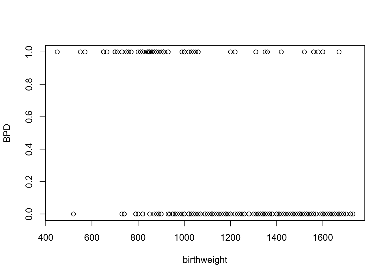
Figure 5.1: Plot of presence of BPD against birthweight for the bpd dataset.
Question
- How does the probability of the development of BPD depend on birthweight?
Response Type
bpd- \(\mathcal{Y} \in \{0,1\}\)
- \({\mathrm E}[Y |f, x] \in [0,1]\)
- \(P_{}\left(y |f, x\right)\)……..Bernoulli?
5.2.2 Dataset B: US Polio Data
Consider the polio data from library gamlss.data.
library( "gamlss.data" )
data( "polio" )
This dataset is a matrix of count data, giving the monthly number of polio cases in United States from 1970 to 1983. We wish to convert this into a usable time series. In other words, we wish to covert this into a matrix with two columns with
- covariate
timein the first column ranging from 1 to 168, starting with January 1970. - response
casesin the second column, indicating the monthly number of polio cases.
We do this as follows
uspolio <- as.data.frame( matrix( c( 1:168, t( polio ) ), ncol = 2 ) )
colnames( uspolio ) <- c("time", "cases")
First, let’s plot the data.
plot( uspolio, type = "h" )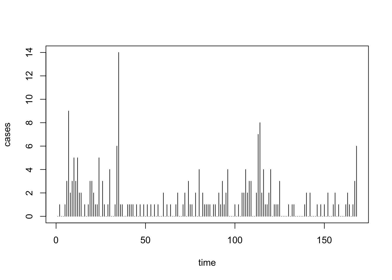
Figure 5.2: Plot of monthly reported number of Polio cases in the US between 1970 and 1983.
Question
- How has Polio incidence changed over time?
Response Type
cases- \(\mathcal{Y} \in \mathbb{N}\)
- \({\mathrm E}[Y |f, x] \in {\mathbb R}_{\geq 0}\)
- \(P_{}\left(y |f, x\right)\)……..Poisson?
5.2.3 Dataset C: Hospital Stay Data
The data, from R package npmlreg, are a subset of a larger data set collected on persons discharged from a selected Pennsylvania hospital as part of a retrospective chart review of antibiotic use in hospitals.
Let’s load the data and then generate a plot.
library(npmlreg)
data(hosp)
plot(hosp[,c("duration","age","temp1","wbc1")])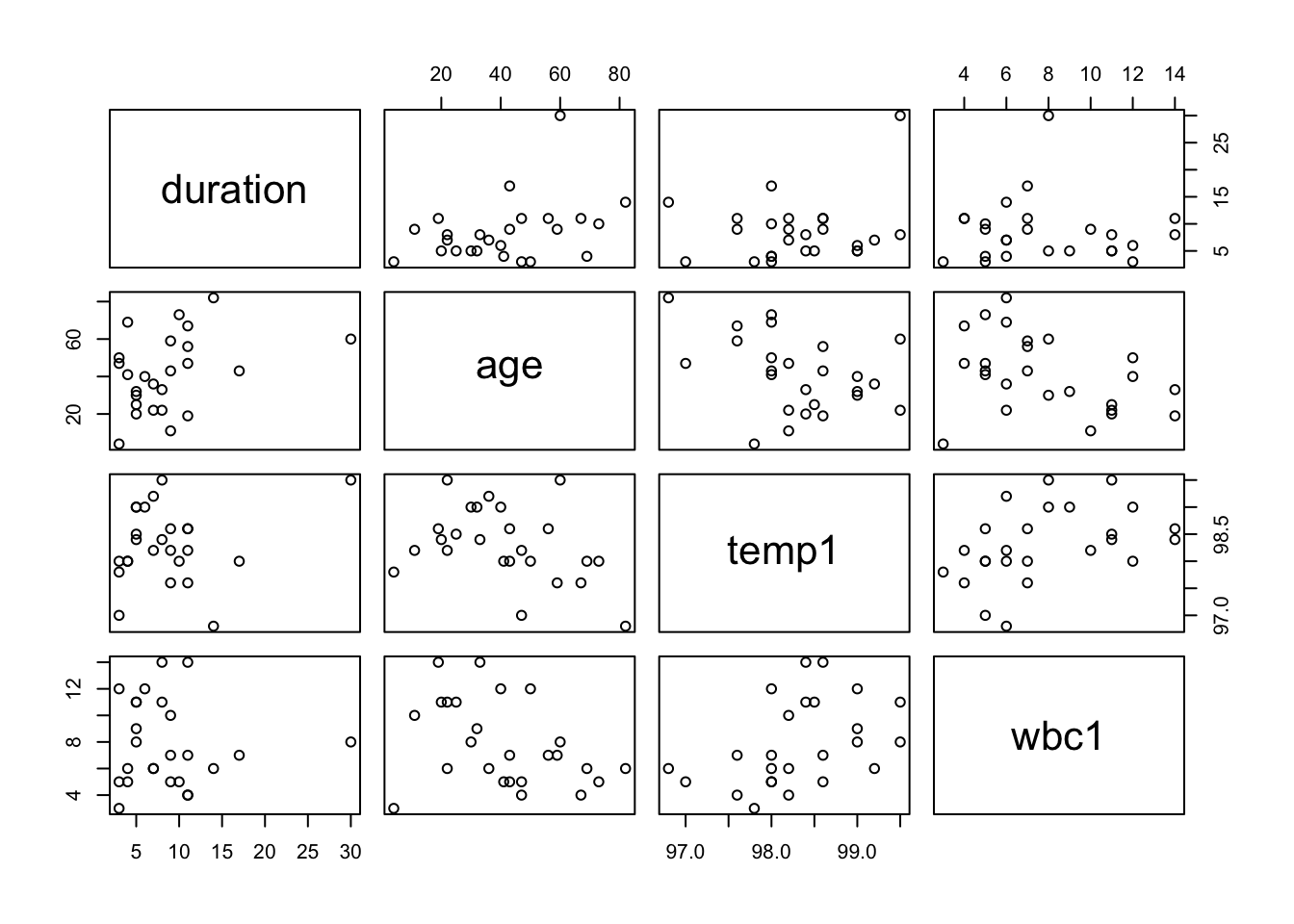
Figure 5.3: Scatter plots of length of hospital stay against three of the most significant covariates.
Question
- How does the duration of a patient’s hospital stay vary, based on data available at the time of admission?
Response Type
duration- \(\mathcal{Y} \in {\mathbb R}_{\geq 0}\)
- \({\mathrm E}[Y |f, x] \in {\mathbb R}_{\geq 0}\)
- \(P_{}\left(y |f, x\right)\)……..Gamma?
5.3 Binary Regression
We consider modelling for the special case in which the data takes on binary values: \(Y \in \left\{0, 1\right\}\).
Binary values usually denote membership or not of some subset of a set: having a disease or not; a credit card transaction being fraudulent or genuine; and so on (can you think of some other examples?).
In this section, we will study this special case, both as important in its own right, and as an introduction to the main ideas of Generalised Linear Models (GLMs), to be discussed in full generality later.
Dataset A (the
bpddataset) considered in Section 5.2.1 is an example in which response variable \(Y\) is binary, taking values 1 or 0, representing presence or absence of BPD respectively.
5.3.1 Modelling Considerations
If a response variable \(Y\) is binary, we know that its expectation must lie in the interval \([0, 1]\), that is \[\begin{equation} {\mathrm E}[Y |f, \boldsymbol{x}] = f(\boldsymbol{x}) \in [0, 1] \end{equation}\]
The only probability distribution available is the Bernoulli distribution, completely characterized by the probability \(\pi\) that \(Y = 1\).
The same quantity, \(\pi\), is also the expectation of \(Y\) under the Bernoulli distribution, that is \[\begin{equation} P_{}\left(Y = 1 |f, \boldsymbol{x}\right) = \pi(\boldsymbol{x}) = {\mathrm E}[Y |f, \boldsymbol{x}] = f(\boldsymbol{x}) \end{equation}\]
Thus the spaces \(\mathcal{Y}\) and \(\mathcal{X}\), along with a probability distribution satisfying Equation (5.4), are in place. The remaining task is to think of a suitable set of possible functions, \(\mathcal{F}\).
A first guess might be to try a linear model: \[\begin{equation} f(\boldsymbol{x}) = \boldsymbol{\beta}^{T}\boldsymbol{x} \end{equation}\] What is wrong with this choice? Well, as you might recall from Section 5.2.1, such a function is unsatisfactory, because for any given value of \(\boldsymbol{\beta}\), there will always be values of \(\boldsymbol{x}\) such that \(\boldsymbol{\beta}^{T}\boldsymbol{x} \not\in [0,1]\). While it may be that there are particular cases where \(\boldsymbol{x}\) only takes on a certain range of values, thereby respecting the constraint on \({\mathrm E}[Y |f, \boldsymbol{x}]\), this cannot be true in general.
The idea that lies behind GLMs is to apply a response function to the linear predictor \(\eta = \boldsymbol{\beta}^{T}\boldsymbol{x}\), in order to constrain it to have the correct range. We thus need to choose a function \(h:{\mathbb R}\to[0,1]\), and then set \[\begin{equation} {\mathrm E}[Y |f, \boldsymbol{x}] = f(\boldsymbol{x}) = h(\boldsymbol{\beta}^{T}\boldsymbol{x}) \end{equation}\] Such a function is shown in Figure 5.4, with the R code used to plot this given below.
eta <- seq( from = -6, to = 6, length = 1000 )
response <- function( x ){ exp(x)/(1+exp(x)) }
plot( eta, response(eta), type = "l",
xlab = expression( eta ), ylab = expression( h(eta) ) )![Graph of a bijective function $\real \rightarrow [0,1]$](_main_files/figure-html/cdf-1.png)
Figure 5.4: Graph of a bijective function \({\mathbb R}\rightarrow [0,1]\)
What possibilities for \(h\) exist? Given the definition, it is apparent that any cumulative distribution function would work, but we would like to be more specific than that.
In fact, there is a standard, or at least most usual, choice: the logistic function (it is this function of \(\eta\) that is plotted in Figure 5.4): \[\begin{equation} h(\eta) = {\frac{e^{\eta}}{1 + e^{\eta}}} = {\frac{1}{1 + e^{-\eta}}} \end{equation}\] This choice for \(h\) leads to the logistic regression model or just logistic model.
5.3.2 The Logistic Regression Model
The logistic regression model consists of three components:
The linear predictor: \[\begin{equation} \eta = \boldsymbol{\beta}^{T}\boldsymbol{x} \end{equation}\]
The logistic response function: \[\begin{equation} {\mathrm E}[Y |f, \boldsymbol{x}] = \pi(\boldsymbol{x}) = f(\boldsymbol{x}) = h(\eta) = {\frac{e^{\eta}}{1 + e^{\eta}}} \end{equation}\]
The probability distribution: \[\begin{equation} Y \sim \text{Bernoulli}(\pi(\boldsymbol{x})) \end{equation}\] or, in other words, \[\begin{equation} P_{}\left(Y = 1 |f, \boldsymbol{x}\right) = P_{}\left(Y = 1 |\boldsymbol{\beta}, \boldsymbol{x}\right) = \pi(\boldsymbol{x}) \end{equation}\]
So, to summarise,
\(Y\) is a binary variable, that is \(Y \in \left\{0,1\right\}\).
At \(\boldsymbol{x} \in \mathcal{X}\) for which the response \(y\) is unobserved, we wish to say something about the distribution of \(y\).
We assume a particular distibutional form for \(y\) (in this case bernoulli), and would like to connect \(\boldsymbol{x}\) with some feature of this distribution, namely the expectation, by a function \(f\).
However, since the expectation must take on a value in \([0,1]\), the standard linear model \(\eta = \boldsymbol{\beta}^Tx\), with potential range \({\mathbb R}\), cannot be used.
We therefore transform the linear predictor using the response function \(h\), which we ensure has potential range \([0,1]\), as required.
5.3.2.1 Reformulations
The following are all equivalent ways of reformulating the logistic model’s relation between \(\pi\) and the linear predictor \(\eta = \boldsymbol{\beta}^{T}\boldsymbol{x}\), providing slightly different perspectives.
The logistic model: \[\begin{equation} \pi(\boldsymbol{x}) = {\frac{e^{\eta}}{1 + e^{\eta}}} \end{equation}\]
A model for the odds: \[\begin{equation} {\frac{\pi(\boldsymbol{x})}{1 - \pi(\boldsymbol{x})}} = e^{\eta} \end{equation}\]
A linear model for the log odds, or logits: \[\begin{equation} \text{logit}(\pi(\boldsymbol{x})) = \log \Big( {\frac{\pi(\boldsymbol{x})}{1 - \pi(\boldsymbol{x})}} \Big) = \eta \end{equation}\]
5.3.2.2 Interpretation of Parameter Values
Suppose we increase the value of the \(a^{\text{th}}\) predictor \(x_{a}\) by \(1\), that is \[\begin{equation} \tilde{\boldsymbol{x}} = \boldsymbol{x} + (0, \ldots, 0, 1, 0, \ldots, 0) \end{equation}\] where the \(1\) is in the \(a^{\text{th}}\) position. Then \[\begin{equation} \text{logit}\left(\pi(\tilde{\boldsymbol{x}})\right) = \boldsymbol{\beta}^{T}\tilde{\boldsymbol{x}} = \boldsymbol{\beta}^{T}\boldsymbol{x} + \beta_{a} \end{equation}\] or (by applying the exponential function to both sides) \[\begin{equation} {\frac{\pi(\tilde{\boldsymbol{x}})}{1 - \pi(\tilde{\boldsymbol{x}})}} = e^{\beta_{a}} {\frac{\pi(\boldsymbol{x})}{1 - \pi(\boldsymbol{x})}} \end{equation}\]
Thus if the \(a^{\text{th}}\) predictor increases in value by \(1\), the odds on \(Y = 1\) change multiplicatively by \(e^{\beta_{a}}\).
5.3.2.3 Practical Example: Dataset A: bpd Data
We will look in detail at modelling the dataset introduced in Section 5.2.1 later. For now, just consider the linear predictor is given by \[\begin{equation} \eta(\boldsymbol{x}) = \beta_{1} + \beta_{2} \texttt{birthweight} \end{equation}\]
The resulting parameter estimates (we will look at parameter estimation in Section 5.3.3) turn out to be \[\begin{align} \hat{\beta}_{1} & = 4.034 \\ \hat{\beta}_{2} & = -0.004229 \end{align}\]
Thus, according to the model, when birth weight increases by \(1\), we estimate that the odds of developing BPD are multiplied by \[\begin{equation} e^{\hat{\beta}_{2}} = e^{-0.004229} = 0.996 \end{equation}\]
that is, according to this model, each additional gram of birth weight reduces the odds of BPD by about \(0.4\%\).
5.3.3 Estimation
We have now set up the logistic model for binary regression.
In practice, of course, we do not know the parameters \(\boldsymbol{\beta}\) (or in other words, the function \(f\in\mathcal{F}\)), and in fact these are usually the quantities in which we are most interested.
We therefore wish to make inferences about them: given data \(\left\{y_{i}\right\}_{i\in[1..n]}\) corresponding to covariate values \(\left\{\boldsymbol{x}_i\right\}_{i\in[1..n]}\), how can we estimate \(\boldsymbol{\beta}\)?
We will use maximum likelihood for this purpose.
The probability of getting the given data \(\left\{y_{i}\right\}\) given knowledge of the \(\left\{\boldsymbol{x}_i\right\}\) and \(\boldsymbol{\beta}\) is \[\begin{eqnarray} P_{}\left(\left\{y_{i}\right\} |\left\{\boldsymbol{x}_i\right\}, \boldsymbol{\beta}\right) & = & \prod_{i} P_{}\left(y_{i} |\boldsymbol{x}_i, \boldsymbol{\beta}\right) \\ & = & \prod_{i} \pi(\boldsymbol{x}_i)^{y_{i}} \, (1 - \pi(\boldsymbol{x}_i))^{1 - y_{i}} \end{eqnarray}\] where we have assumed that:
given the \(\left\{\boldsymbol{x}_i\right\}, i = 1,...,n\), our knowledge of any particular \(y_{k}, k \in \{1,...,n\}\) is not altered by knowledge of other \(y_{j}\) for \(j \neq k\);
given \(\boldsymbol{x}_k\), our knowledge of \(y_{k}\) is not altered by knowledge of other \(\boldsymbol{x}_j\) for \(j \neq k\).
Note that these are distinct assumptions, the first corresponding to the \(y_{i}\) being independent of each other.62
Abbreviating \(\pi(\boldsymbol{x}_i)\) by \(\pi_{i}\), the log likelihood is thus \[\begin{eqnarray} l\left(\boldsymbol{\beta} ; \left\{\boldsymbol{x}_i\right\}, \left\{y_{i}\right\}\right) & = & \log P_{}\left(\left\{y_{i}\right\} |\left\{\boldsymbol{x}_i\right\}, \boldsymbol{\beta}\right) \\ & = & \sum_{i} \Big[ y_{i}\log \pi_{i} + (1 - y_{i})\log (1 - \pi_{i}) \Big] \\ & = & \sum_{i} \Big[ y_{i}\log {\frac{\pi_{i}}{1 - \pi_{i}}} + \log (1 - \pi_{i}) \Big] \\ & = & \sum_{i} \Big[ y_{i}\boldsymbol{\beta}^{T}\boldsymbol{x}_i - \log (1 + e^{\boldsymbol{\beta}^{T}\boldsymbol{x}_i}) \Big] \end{eqnarray}\]
where for the final line we note that \[\begin{equation} 1 - \pi_i = 1 - \frac{e^{\boldsymbol{\beta}^T\boldsymbol{x}_i}}{1 + e^{\boldsymbol{\beta}^T\boldsymbol{x}_i}} = \frac{1 + e^{\boldsymbol{\beta}^T\boldsymbol{x}_i} - e^{\boldsymbol{\beta}^T\boldsymbol{x}_i}}{1 + e^{\boldsymbol{\beta}^T\boldsymbol{x}_i}} = \frac{1}{1 + e^{\boldsymbol{\beta}^{T}\boldsymbol{x}_i}} \end{equation}\]
5.3.4 The Score Function
The score function is given by \[\begin{equation} \boldsymbol{S}(\boldsymbol{\beta}) = {\frac{\partial l}{\partial\boldsymbol{\beta}^{T}}}(\boldsymbol{\beta}) = \nabla l\left(\boldsymbol{\beta}\right) \tag{5.5} \end{equation}\] that is, the derivative of the log-likelihood function with respect to \(\boldsymbol{\beta}^T\).
The Maximum Likelihood Estimate (MLE) of \(\boldsymbol{\beta}\), denoted \(\hat{\boldsymbol{\beta}}\), will, for well-behaved likelihoods, satisfy the equation \[\begin{equation} \boldsymbol{S}(\hat{\boldsymbol{\beta}}) = 0 \tag{5.6} \end{equation}\] Equation (5.6) is known as the score equation.
To be a maximum, we must also have \[\begin{equation} \boldsymbol{H} ( l(\hat{\boldsymbol{\beta}}) ) \leq 0 \tag{5.7} \end{equation}\] where \(\leq 0\) here denotes negative semidefinite63, and \(\boldsymbol{H}\) denotes the Hessian matrix64: \[\begin{equation} \boldsymbol{H} ( l\left(\boldsymbol{\beta}\right) ) = { \frac{\partial^{2}l}{\partial\boldsymbol{\beta}\partial\boldsymbol{\beta}^{T}}}(\boldsymbol{\beta}) \end{equation}\] that is, the second derivative of the log-likelihood function.
5.3.4.1 For Logistic Regression…
- For logistic regression, the score function is given by \[\begin{eqnarray} \boldsymbol{S}(\boldsymbol{\beta}) & = & \sum_{i} \Big[ y_{i}\boldsymbol{x}_i - {\frac{e^{\boldsymbol{\beta}^{T}\boldsymbol{x}_i}}{1 + e^{\boldsymbol{\beta}^{T}\boldsymbol{x}_i}}}\boldsymbol{x}_i \Big] \\ & = & \sum_{i} (y_{i} - \pi_{i})\boldsymbol{x}_i \end{eqnarray}\] where the first line is obtained by use of the chain rule with \(u = 1 + e^{\boldsymbol{\beta}^T\boldsymbol{x}_i}\): \[\begin{equation} {\frac{\partial}{\partial\boldsymbol{\beta}^{T}}} \log(1 + e^{\boldsymbol{\beta}^T\boldsymbol{x}_i}) = \frac{1}{1 + e^{\boldsymbol{\beta}^T\boldsymbol{x}_i}}\boldsymbol{x}_i e^{\boldsymbol{\beta}^T\boldsymbol{x}_i} \end{equation}\]
5.3.4.2 Solving The Score Equation
The score equation (for binary regression, or more generally) \[\begin{equation} \boldsymbol{S}(\hat{\boldsymbol{\beta}}) = 0 \end{equation}\] is a system of nonlinear equations of \(\hat{\boldsymbol{\beta}}\) (the parameters).
In general, no analytical solution exists, so we need to use a numerical method to find a solution. We thus need an algorithm to perform the task we have set ourselves, of finding the MLE, and, in the interests of time efficiency, a computer to perform the computations. There are two broad classes of algorithm that are relevant:65
Optimization algorithms, which will attempt to find a global or local minimum of \(l\);
Nonlinear equation solvers, which will attempt to solve \(\boldsymbol{S}(\hat{\boldsymbol{\beta}}) = 0\).
The most common method in our context is iterative weighted least squares (IWLS)66.
5.3.4.2.1 Exception
An exception to the need for an algorithm is the case with \(p = 2\), \(x_{1} = 1\), and \(x_{2}\in \{0, 1\}\) (that is, a single binary covariate). In this case, an analytical solution is available. It is left as an exercise for the reader67.
5.3.5 Logit and Probit
Are there any alternatives to the logistic function? The answer, of course, is yes: any cdf will do. In practice, the second most popular response function for binary regression is the cdf of the standard normal distribution \[\begin{eqnarray} \pi(\boldsymbol{x}) & = & \Phi(\boldsymbol{\beta}^{T}\boldsymbol{x}) \\ \Phi^{-1}(\pi(\boldsymbol{x})) & = & \boldsymbol{\beta}^{T}\boldsymbol{x} \end{eqnarray}\]
The inverse, \(\Phi^{-1}\), is known as the probit function. A comparison of the logit and probit models is presented in the table in Figure 5.5.
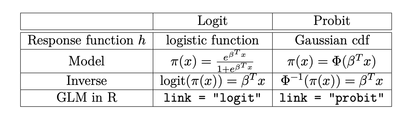
Figure 5.5: A comparison of the logit and probit models.
5.3.5.1 Practical Example: Dataset A
We fit a logit and a probit model to the the
bpddata introduced in Section 5.2.1.This uses the
glmcommand from R packageSemiPar, which is the general R command for fitting a generalised linear model.Notice, however, similarities and differences with the
lmcommand in R, and also where we inform R of whether we wish to fit alogitor aprobitmodel.
# Load the data.
library( SemiPar )
data( bpd );
attach( bpd )

# Fit logistic regression model
fitl <- glm( BPD ~ birthweight, family = binomial( link = logit ) )
fitl
##
## Call: glm(formula = BPD ~ birthweight, family = binomial(link = logit))
##
## Coefficients:
## (Intercept) birthweight
## 4.034291 -0.004229
##
## Degrees of Freedom: 222 Total (i.e. Null); 221 Residual
## Null Deviance: 286.1
## Residual Deviance: 223.7 AIC: 227.7# Comparison with probit link
fitp <- glm( BPD ~ birthweight, family = binomial( link = probit ) )
fitp##
## Call: glm(formula = BPD ~ birthweight, family = binomial(link = probit))
##
## Coefficients:
## (Intercept) birthweight
## 2.276856 -0.002383
##
## Degrees of Freedom: 222 Total (i.e. Null); 221 Residual
## Null Deviance: 286.1
## Residual Deviance: 225.4 AIC: 229.4Note that although the parameter values are quite different, if we plot the expectation functions, we can see that they are very similar. We also add on the regression line from a standard linear model for comparison purposes. Notice how the logit and probit models are constrained between 0 and 1 (and would be even if you extended the x-axis beyond the visualised range), however, the linear model visually predicts outside this range on the displayed plot.
# Plot the bpd dataset.
plot( birthweight, BPD )

# Try a standard regression line using lm command:
abline( lm( BPD ~ birthweight ), col = 3 )

# Include fitted pi(x_i) into plot
lines( birthweight[order( birthweight )], fitl$fitted[order( birthweight )] )
lines( birthweight[order( birthweight )], fitp$fitted[order( birthweight )],
       col = 2 )

# Add a legend
legend( x = 1300, y = 0.8, col = 1:3, lty = 1,
        legend=c( "logit", "probit", "linear model" ) )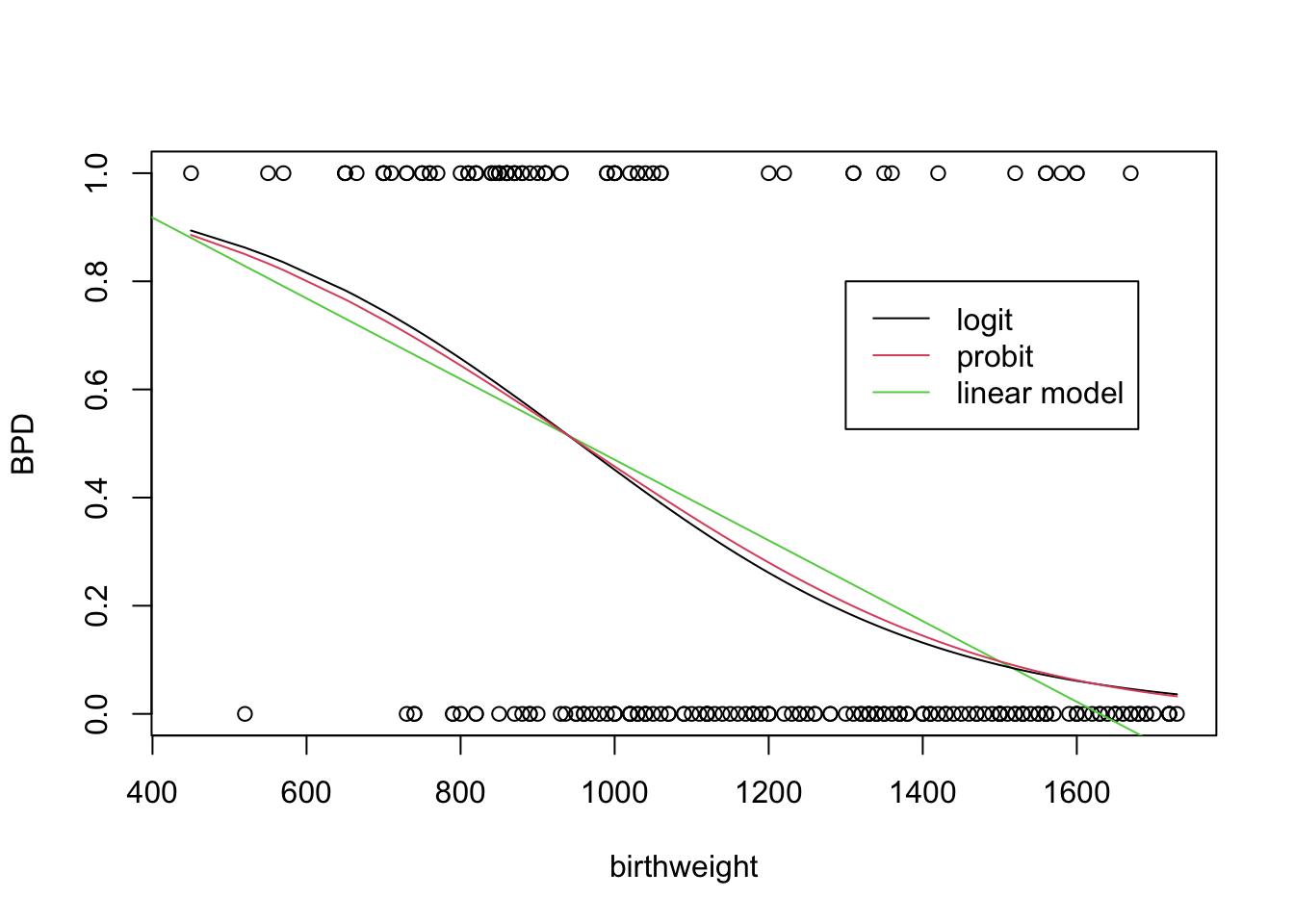
The notion of variables (and random variables) was discussed in Q1-1.↩︎
The notation \(P_{}\left(y | \ldots\right)\) will be used to mean the probability of \(Y = y\) in the case that \(\mathcal{Y}\) is countable, and to represent the density \(P_{}\left(Y\in[y, y + dy]\right)/dy\) in the case that \(\mathcal{Y}\) is continuous.↩︎
Here \(K\) represents all the other knowledge, e.g. values of other parameters, that may be relevant. We will, however, often drop the \(K\) for notational convenience.↩︎
The notation \([m..n]\) will indicate all natural numbers \(i\) such that \(m \leq i \leq n\).↩︎
Recall that the space of predictors is not the same as the space of covariates. For example, there might only be one covariate, \(z \in {\mathbb R}\), but many predictors, corresponding, for example, to \(x_{a} = z^{a - 1}\), \(a\in [1..p]\).↩︎
The word assumption is a bad one. It sounds as if we are assuming that something is true when in reality, it might be false. However, independence is not a property of the world at all. For example, when two people, A and B, walk into a building one after another, the propositions A carried an umbrella and B carries an umbrella are not independent if I am inside the building and do not know whether it is raining or not, because the first being true suggests that it is raining, which increases the probability of the second being true. However, if I know (condition on the fact) that it is raining, then they are independent, or nearly so, because knowledge that one is true does not affect the probability of the second. Nothing changed in the world, only in my knowledge of it. Thus independence says that given the conditioning knowledge, a change in our knowledge of one quantity does not affect our knowledge of another. Usually independence is used because we judge the relevant changes in knowledge to be small, so that it is a good approximation to our state of knowledge, and because it simplifies calculations greatly.↩︎
Recall: A symmetric matrix \(A\) is said to be positive definite if and only if \(b^TAb > 0\) for all vectors \(b \neq 0\), and positive semi-definite if the inequality is not strict (i.e., \(\geq\)). Similarly, \(A\) is said to be negative definite if and only if \(b^TAb < 0\) for all vectors \(b \neq 0\), and negative semi-definite if the inequality is not strict.↩︎
Note that equations (5.6) and (5.7) are not sufficient for \(\hat{\boldsymbol{\beta}}\) to be the MLE. The log likelihood may have many local maxima, all of which will satisfy both these equations, yet, generically, only one can be the global maximum. In fact, these equations are not necessary either: the maximum may not occur at a differentiable point, usually because it occurs at a boundary (e.g. \(e^{-\boldsymbol{x}}\) on \({\mathbb R}_{\geq 0}\)), but not always (e.g. \((1 - |\boldsymbol{x}|)\) on \([-1, 1]\)). Note too that if the second derivative is not negative definite, there will be an infinite number of maxima in the flat direction.↩︎
In practice, the former are quite often implemented via the latter, although this need not be the case. There are advantages to optimization algorithms that do not require derivatives.↩︎
This name will be demystified later when we describe the method.↩︎
Q5-1c, in fact.↩︎