Chapter 7 Generalised Linear Models

7.1 Setting The Scene

We are given:

Predictors $\boldsymbol{x} \in \mathcal{X}\subseteq{\mathbb R}^p$: recall that in general these will be a function of the actual covariates $\boldsymbol{z}$, for example $\boldsymbol{x} = \boldsymbol{\varphi}(\boldsymbol{z})$. The predictors are numerical; either naturally, or because they are an encoding of categorical variables.
A response $y \in \mathcal{Y} \subseteq {\mathbb R}$. This may be numerical; continuous or discrete, or it may be binary. For now, we do not consider nominal responses with more than two values, for example $Y \in \left\{\text{red, green, blue}\right\}$⁷⁰.

We suppose that there is some functional relationship between the predictors and the response, i.e. that $P_{}\left(y |\boldsymbol{x}, f\right) = P_{}\left(y |f(\boldsymbol{x})\right)$, with ${\mathrm E}[Y |\boldsymbol{x}, f] = f(\boldsymbol{x})$, for some $f\in\mathcal{F}$, a suitable set of possible functions.

One class of models of functional relationships, defined via a set of possible functions $\mathcal{F}$ and a set of possible probability distributions whose means will be controlled by those functions, are the generalised linear models (GLMs), which we now define.

7.2 Definition

A GLM is specified through the following components:

A linear predictor: \[\begin{equation} \eta = \boldsymbol{\beta}^{T}\boldsymbol{x} \end{equation}\]
An injective response function $h$, such that \[\begin{equation} \mu = {\mathrm E}[Y |\boldsymbol{x}, \boldsymbol{\beta}] = h(\eta) = h(\boldsymbol{\beta}^{T}\boldsymbol{x}) \end{equation}\] Equivalently, one can write \[\begin{equation} g(\mu) = \boldsymbol{\beta}^{T}\boldsymbol{x} \end{equation}\] where $g = h^{-1}$ is the link function.
The distributional assumption: our knowledge of $Y$ given $\boldsymbol{x}$ and $\boldsymbol{\beta}$ is described by an EDF with parameters that depend on $\boldsymbol{x}$ and $\boldsymbol{\beta}$: \[\begin{equation} P_{}\left(y |\boldsymbol{x}, \boldsymbol{\beta}\right) = P_{}\left(y |\theta(\boldsymbol{x}, \boldsymbol{\beta}), \phi(\boldsymbol{x}, \boldsymbol{\beta})\right) = \exp \Big( \frac{y\theta - b(\theta)}{\phi} + c(y, \phi) \Big) \end{equation}\] In addition, values of $Y$ for different $\boldsymbol{x}$ and $\boldsymbol{\beta}$ will be assumed to be independent of each other and other $\boldsymbol{x}$ values (but not $\boldsymbol{\beta}$), that is: \[\begin{equation} P_{}\left(\left\{y_{i}\right\} |\left\{\boldsymbol{x}_{i}\right\}, \boldsymbol{\beta}\right) = \prod_{i=1}^n P_{}\left(y_{i} |\boldsymbol{x}_{i}, \boldsymbol{\beta}\right) \end{equation}\] where $\left\{y_{i}, i = 1,...,n\right\}$ are response data given the $\left\{\boldsymbol{x}_i, i = 1,...,n\right\}$.

7.3 The Natural/Canonical Link

There is one choice of response (or equivalently link) function that greatly simplifies the formulism. This is known as the natural link or canonical link, although in practice it does not always seem that natural at all.⁷¹

Recall that we have both: \[\begin{alignat}{4} \mu & = {\mathrm E}[Y |\theta, \phi] && = b'(\theta) \tag{7.1} \\ \mu & = {\mathrm E}[Y |\boldsymbol{x}, \boldsymbol{\beta}] && = h(\boldsymbol{\beta}^T\boldsymbol{x}) = h(\eta) \tag{7.2} \end{alignat}\] with Equation (7.1) holding as a result of $P_{}\left(y |\theta, \phi\right)$ following an EDF distribution, and Equation (7.2) holding by definition for a GLM. Following Equations (7.1) and (7.2), we have that \[\begin{equation} \theta = (b')^{-1}(\mu) = (b')^{-1}(h(\boldsymbol{\beta}^{T}\boldsymbol{x})) \end{equation}\] The natural link is the choice $h = b'$, or equivalently $g = (b')^{-1}$, resulting in the equation \[\begin{equation} \theta = \boldsymbol{\beta}^T\boldsymbol{x} = \eta \tag{7.3} \end{equation}\] It is clear that this will simplify the formulism. Other links may still be used if needed, especially since the natural link often has undesirable properties.

7.3.1 Examples

We now apply the preceding theory to our three examples.

7.3.1.1 Poisson

From Section 6.2.3.1: $\mu = b'(\theta) = e^\theta$.
The natural response function is thus $\mu = h(\eta) = e^\eta$.
Natural link is therefore $\eta = g(\mu) = \log \mu$.

7.3.1.2 Bernoulli

From Section 6.2.3.2: $\mu = b'(\theta) = e^\theta/(1+e^\theta)$.
The natural response function is thus $\mu = h(\eta) = e^\eta/(1+e^\eta)$.
Natural link is therefore $\eta = g(\mu) = \log ( \mu / (1-\mu))$, i.e. the logit function.

7.3.1.3 Gaussian

From Section 6.2.3.3: $\mu = b'(\theta) = \theta$.
The natural response function is thus $\mu = h(\eta) = \eta$.
Natural link is therefore $\eta = g(\mu) = \mu$.

7.4 Grouped Data

We have seen that for a GLM, the expectation of the response is a function of $\theta$ only, which in turn is a function of $\boldsymbol{\beta}$ and $\boldsymbol{x}$ via $\eta = \boldsymbol{\beta}^{T}\boldsymbol{x}$.

In principle, the dispersion $\phi$ may also be a function of $\boldsymbol{x}$ or otherwise vary from data point to data point. In practice, however, it is usually assumed to be constant: e.g. for Poisson, where $\phi = 1$, or Gaussian, where $\phi = \sigma^{2}$. The most common exception is the case of grouped data, where multiple replicates may be observed for a given $\boldsymbol{x}$.

7.4.1 Grouped Binary Data

Let $\pi(\boldsymbol{x}) = \frac{e^{\boldsymbol{\beta}^{T}\boldsymbol{x}}}{1 + e^{\boldsymbol{\beta}^{T}\boldsymbol{x}}}$, and suppose that there are several binary values for each $\boldsymbol{x}$, that is we have data \[\begin{equation} \left\{(\boldsymbol{x}_{i}, \left\{y_{ir}\right\}_{r\in[1..m_{i}]})\right\}_{i\in[1..n]} \end{equation}\] where $m_{i}$ is the number of replicates for group $i$, indexed by $r$; $n$ is the number of groups, and $M = \sum_{i} m_{i}$ is the total sample size.

If our data consists just of the counts \[\begin{equation} \tilde{y}_{i} \triangleq \sum_{r = 1}^{m_{i}} y_{ir} \end{equation}\] then while the individual $y_{ir}$ are Bernoulli-distributed with parameter $\pi(\boldsymbol{x}_{i})$, the $\tilde{y}_{i}$ are binomially distributed, with parameters $m_{i}$ and $\pi(\boldsymbol{x}_{i})$, that is \[\begin{equation} \tilde{Y}_{i} = \sum_{r} Y_{ir} \sim \text{Bin}(m_{i}, \pi(\boldsymbol{x}_{i})) \end{equation}\]

It turns out, however, to be more convenient to model not the counts themselves, but the proportions or averages, that is \[\begin{equation} Y_{i} \triangleq \bar{Y}_{i} = \frac{1}{m_{i}} \sum_{r} Y_{ir} \sim \frac{1}{ m_{i}} \text{Bin}(m_{i}, \pi(\boldsymbol{x}_{i})) \end{equation}\] where the distribution, corresponding to a binomial variable divided by the number of trials, is known as the scaled or rescaled binomial distribution.

The reason that it is more convenient to use the $y_{i}$ instead of the $\tilde{y}_{i}$ is because the expectation still takes the form: \[\begin{equation} {\mathrm E}[Y |m, \boldsymbol{x}] = \frac{1}{ m} m \pi(\boldsymbol{x}) = \pi(\boldsymbol{x}) \end{equation}\] meaning that the expectation function can still be modelled in the same way as for binary regression, using, for example, the logistic function. There is thus no need to include $m$ at the level of the expectation, only in the distribution.⁷²

We have been acting as if the model resulting from this procedure is a GLM. We have seen at the level of the expectation that this is true, but what about the distribution? Is the rescaled binomial distribution an EDF? The answer is yes, as follows. \[\begin{eqnarray} P_{}\left(y |m, \pi\right) & = & P_{}\left(\text{$my$ `successes' in $m$ `trials'} |m, \pi\right) \\ & = & {m \choose my} \pi^{my} (1 - \pi)^{m - my} \\ & = & \exp \left\{ my \log\pi + (m - my)\log(1 - \pi) + \log {m\choose my} \right\} \\ & = & \exp \left\{ {m( y ( \log{\pi} - \log(1 - \pi) ) } + \log(1 - \pi) ) + c(y, \frac{1}{m}) \right\} \\ & = & \exp \left\{ \frac{y \log \frac{\pi}{ 1 - \pi} + \log(1 - \pi)}{\frac{1}{ m}} + c(y, \frac{1}{m}) \right\} \end{eqnarray}\]

Thus the rescaled binomial distribution is an EDF, with \[\begin{eqnarray} \theta & = & \log \frac{\pi}{ 1 - \pi} \\ \phi & = & \frac{1}{ m} \end{eqnarray}\]

Thus $\theta$ is the same as in the Bernoulli case, while $\phi = 1$ is replaced by $\phi = 1 / m$. The dispersion thus depends on $m$, and so if different groups $i$ have different numbers of replicates $m_{i}$, the dispersion will vary with $i$: \[\begin{equation} \phi_{i} = \frac{1 }{ m_{i}} \end{equation}\]

7.4.2 Example: Rainfall Data

We consider rainfall data recorded in Tokyo in the first 11 days of the year 1983. For each day, we know whether it rained ($z_i=1)$ or did not rain ($z_i=0$) on that day, as given by the table in Figure 7.1.

Figure 7.1: Rainfall data in Tokyo in the first 11 days of the year 1983.

The goal is to find a model which predicts the probability of rain on day $i+1$ based on the rainfall on day $i$, which is given by $z_i$. Based on this binary data, we previously defined the response $y_i=z_{i+1}$, $i=1, \ldots, 10$, so that we could write the data in the form given by the table in Figure 7.2.

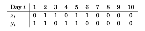
Figure 7.2: Rainfall data in Tokyo for the first 10 days of the year 1983 along with data about whether it rained the following day.

Instead of treating the response variable as a binary response to a binary covariate, with the data consisting of the values of this covariate for rainfall each day and the values of the response for rainfall the day after, we now treat the response as a rescaled binomial variable giving the proportion of response values $1$ corresponding to each of the two possible values of the covariate.

The data therefore corresponds to the table in Figure 7.3.

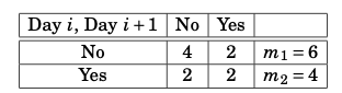
Figure 7.3: Grouped rainfall data.

The sample size is thus $m_{1} + m_{2} = M = 10$, while the number of groups $n = 2$. We can denote the two values of the covariate corresponding to the two groups as $z_{1} = 0$ and $z_{2} = 1$. We then have the grouped data: \[\begin{align} z_{1} = 0 & \qquad & y_{1} = \frac{2}{6} = \frac{1}{3} & \qquad & m_{1} = 6 \\ z_{2} = 1 & & y_{2} = \frac{2}{4} = \frac{1}{2} & & m_{2} = 4 \end{align}\]

The model will be \[\begin{equation} Y_{i} \sim \frac{1}{m_{i}} \text{Bin}(m_{i}, \pi_{i}) \end{equation}\] where $\pi_{i} = \pi(x_{i}) = \frac{e^{\beta_{1} + \beta_{2}z_{i}}}{1 + e^{\beta_{1} + \beta_{2}z_{i}}}$, with $i\in\left\{1, 2\right\}$. This gives rise to the probability of the data: \[\begin{equation} P_{}\left(\left\{y_{i}\right\} |\left\{m_{i}\right\}, \left\{x_{i}\right\}, \boldsymbol{\beta}\right) = \prod_{i} {m_{i} \choose m_{i}y_{i}} \pi_{i}^{m_{i}y_{i}} (1 - \pi_{i})^{m_{i} - m_{i}y_{i}} \end{equation}\]

Estimation for this case is examined in Question 7-1.

7.4.3 General Case

If $P_{}\left(y_{r} |\theta, \phi\right)$ is an EDF for each $r\in[1..m]$, with natural parameter $\theta$, log normalizer $b$, dispersion $\phi$, and function $c$, then the grouped data, \[\begin{equation} y \triangleq \bar{y} = \frac{1}{ m} \sum_{r} y_{r} \end{equation}\] has a probability distribution that is also an EDF. This EDF has the same natural parameter $\theta$ and log-normalizer $b$ as the original distribution, but $\phi$ is replaced by $\frac{\phi}{m}$ and the function $c$ may be different and a function of $m$.

In general, it is advisable to group data as far as possible because:

it simplifies the equations.
it improves speed of convergence and hence computation time.
some theory only holds when $m \gg 1$.

However, grouping may be impossible for continuous predictors.

You may consider these next term.↩︎
Perhaps it would be better called the easy link!↩︎
Note that there is still a conditioning on known $m$ in the expression for expectation, so this statement is different from knowing the proportion without knowing the number of replicates, which would require treating $m$ as a nuisance parameter, either via profile likelihoods, or by assigning a prior and integrating it out.↩︎