Chapter 1 Motivation, Introduction and Review
1.1 Course Content
In these lectures, we are going to discuss:
Categorical Data Analysis: we will study use of
Contingency Tables: We will learn about the different types of possible associations between two or more categorical variables, before learning how to make inferences about such associations. As part of this, we will discover the importance of different sampling schemes and learn how to make statements about associations between categorical variables utilising odds and odds ratios.
Log-Linear Models: A way of modelling the counts for categorical data represented in contingency tables, with the categorical variables themselves being the predictors. The construction of such models is highly useful for testing and representing (modelling) the associations between the categorical variables themselves.
Generalised Linear Models: a broad class of models permitting
the response variable \(y\) to come from a space that is a subset of the real numbers, e.g. the positive real numbers, or countable subsets such as \(\mathbb{N}\) or the set \(\left\{0, 1\right\}\).
a larger set \(\mathcal{F}\) of functions for making predictive statements about response \(y\) based on predictor variables \(\boldsymbol{x}\) (not just linear combinations of the predictors). These will be formed by combining the linear functions used in linear models with nonlinear maps from \({\mathbb R}\to{\mathbb R}\).
consideration of general families of probability distributions for response \(y\) (not just normal).
We will then go on to develop the standard tools of classical statistics:
Estimators for the parameters of the model: we will use maximum likelihood.
Sampling distributions for these estimators, either exactly or approximately, and especially their expectations and variances.
Statistical tests and confidence intervals; predictions with corresponding prediction intervals.
Measures of “goodness-of-fit” for model selection.
1.1.1 Section Overview
In the rest of this introductory chapter, we present a review of some of the most useful material from previous prerequisite courses. At the end of this section, there is a set of references for the course, which will allow you to take your study of Advanced Statistical Modelling deeper than just being restricted to what is contained in these lecture notes alone (brilliant though they are, of course!).
1.2 Statistical Inference II: A Review
This section summarises some of the key topics from Statistical Inference II. Review the corresponding lecture notes (particularly the Chapter on Likelihood Inference) for further detail.
1.2.1 Statistical Inference
A statistical model (also known as a family of distributions) is a set of distributions (or densities) \(M\).
A parametric model is any model \(M\) that can be parameterised by a finite number of parameters.
1.2.2 Likelihood Inference
1.2.2.1 Maximum Likelihood Estimation
Suppose data \(\boldsymbol{X}=(X_1,...,X_n)^T\) has joint density \(f(\boldsymbol{x};\theta)\). Given a statistical model parameterised by a fixed and unknown scalar \(\theta \in \Omega \subseteq {\mathbb R}\), the likelihood function, \(L(\theta)\), is the probability (density) of the observed data considered as a function of \(\theta\) \[\begin{equation} L(\theta) = L(\theta; \boldsymbol{x}) = f(\boldsymbol{x}; \theta) \end{equation}\] and the log-likelihood function is its logarithm \[\begin{equation} l(\theta) \equiv l(\theta;\boldsymbol{x}) = \log L(\theta) = \log f(\boldsymbol{x};\theta) \end{equation}\]
The Maximum Likelihood Estimate (MLE) \(\hat{\theta}\) for \(\theta\) given the data \(\boldsymbol{x}\) is the value of \(\theta\) which maximises the likelihood over the parameter space \[\begin{equation} \hat{\theta} = {\arg \max}_{\theta \in \Omega} l(\theta) = {\arg \max}_{\theta \in \Omega} L(\theta) \end{equation}\]
If \(X_1,...,X_n\) are i.i.d. then \[\begin{eqnarray} L(\theta) & = & f(x_1,...,x_n; \theta) = \prod_{i=1}^n f(x_i;\theta) \\ l(\theta) & = & \log \prod_{i=1}^n f(x_i;\theta) = \sum_{i=1}^n \log f(x_i;\theta) \end{eqnarray}\]
1.2.2.2 Properties of the MLE
If \(\hat{\theta}\) is the MLE of \(\theta\) and \(\phi = g(\theta)\) is a function of \(\theta\), then \(\hat{\phi} = g(\hat{\theta})\).
A statistic \(S = S(\boldsymbol{X})\) is a sufficient statistic for \(\theta\) if the conditional distribution of \(\boldsymbol{X} |S = s\) does not depend on \(\theta\).
Factorisation Theorem: A statistic \(S = S(\boldsymbol{X})\) is sufficient for \(\theta\) if and only if there exist functions \(g(S,\theta)\) and \(h(\boldsymbol{X})\) such that for all \(\boldsymbol{X}\) and \(\theta\): \[\begin{equation} f(\boldsymbol{X};\theta) = g(S, \theta) \, h(\boldsymbol{X}) \end{equation}\] where \(h(\boldsymbol{X})\) does not depend on \(\theta\).
If \(S=S(\boldsymbol{X})\) is a sufficient statistic of \(\boldsymbol{x}\) for \(\theta\), and the MLE \(\hat{\theta}\) of \(\theta\) exists, then \[\begin{equation} \hat{\theta}(\boldsymbol{x}) = \hat{\theta}(s(\boldsymbol{x})) \end{equation}\]
1.2.3 (Frequentist) Hypothesis Testing
1.2.3.1 Hypotheses
A hypothesis is any statement about the probability model \(M = \{f(\boldsymbol{x} |\theta) |\theta \in \Omega \}\) generating the data. When the probability distribution of the model is fixed, then a hypothesis is simply a statement about the parameter \(\theta\)1.
A hypothesis is simple if it completely specifies the associated probability distribution, \(f(\boldsymbol{x} |\theta)\). Otherwise, a hypothesis is called composite (or compound).
The null hypothesis, \(\mathcal{H}_0\), is a conservative hypothesis, not to be rejected unless evidence from the data is clear. The alternative hypothesis, \(\mathcal{H}_1\), specifies a particular departure from the null hypothesis that is of interest.
A hypothesis test is a procedure for deciding whether to reject \(\mathcal{H}_0\) or not.
1.2.3.2 Hypothesis Test
We define a test by a critical or rejection region, \(\mathcal{R}\), which partitions the sample space \(\mathcal{X}\) such that:
- If \(\boldsymbol{x} = (x_1,...,x_n) \in \mathcal{R}\), then we say that the test rejects \(\mathcal{H}_0\).
- If \(\boldsymbol{x} = (x_1,...,x_n) \notin \mathcal{R}\), then the test fails to reject \(\mathcal{H}_0\).
A test statistic, \(T\), is a statistic derived from the sample used in hypothesis testing. The sampling distribution of \(T\) under the null hypothesis is known as the null distribution.
We can define the rejection region in terms of values of the test statistic \[\begin{equation} \mathcal{R} = \{ \boldsymbol{x} |T(\boldsymbol{x}) \in \mathcal{T} \} \end{equation}\] for some set of possible values \(\mathcal{T}\) . Usually, once we find a test statistic, we just ignore the original critical region and just focus on whether or not \(T\) is in \(\mathcal{T}\) or not.
Assuming \(\mathcal{H}_0\) is true, we can construct the sampling distribution for \(T\), \(f_T (t)\) – known as the null distribution for \(T\) – and define \(\mathcal{R}\) as corresponding to the set of values of \(T\) which are “sufficiently unlikely” to occur under \(\mathcal{H}_0\) to cause us to reject \(\mathcal{H}_0\).
1.2.3.3 Significance, Power and \(p\)-values
For a simple null hypothesis, the significance level of a test is the probability \[\begin{equation} \alpha = P(\textrm{reject} \, \mathcal{H}_0 |\mathcal{H}_0 \, \textrm{true}) \end{equation}\] Then \[\begin{equation} \mathcal{R} = \{\boldsymbol{x} |P(T(\boldsymbol{x}) \in \mathcal{T} |\mathcal{H}_0) \leq \alpha \} \end{equation}\]
Two errors can arise in hypothesis testing:
- Reject \(\mathcal{H}_0\) when \(\mathcal{H}_0\) true - a type I error, occurs with probability \(\alpha\). If \(\mathcal{H}_0\) is simple, this is the usual significance level.
- Do not reject \(\mathcal{H}_0\) when \(\mathcal{H}_1\) true - a type II error, occurs with probability \(\boldsymbol{\beta}\).
Given an observed sample \(\boldsymbol{X} = \boldsymbol{x}\) and a simple null hypothesis \(\mathcal{H}_0\), the \(p\)-value or observed significance is the smallest value of \(\alpha\) for which we would reject the null hypothesis \(\mathcal{H}_0\) on the basis of the data \(\boldsymbol{x}\).
A \(p\)-value is the probability of observing a test statistic \(T\) “at least as extreme” as the one observed, \(t\), under the null distribution: \[\begin{equation} p=P(T \, \textrm{“at least as extreme as”} \, t |\mathcal{H}_0) \end{equation}\] What “extreme” is depends on the nature of the alternative hypothesis \(\mathcal{H}_1\) and the \(p\)-value quantifies the extent to which the null hypothesis is violated.
There is a duality of confidence intervals and hypothesis tests2.
- A \(100(1 - \alpha)\%\) confidence region for a parameter \(\theta\) consists of all of those values of \(\theta_0\) for which the hypothesis that \(\theta=\theta_0\) will not be rejected at level \(\alpha\).
- Equivalently, the hypothesis that \(\theta = \theta_0\) is accepted if \(\theta_0\) lies in the same confidence region.
- A \(100(1 - \alpha)\%\) confidence region for a parameter \(\theta\) consists of all of those values of \(\theta_0\) for which the hypothesis that \(\theta=\theta_0\) will not be rejected at level \(\alpha\).
1.2.3.4 Likelihood Ratio Tests
Given a sample \(\boldsymbol{X} = (X_1,..., X_n)\) and the general hypotheses \(\mathcal{H}_0\) and \(\mathcal{H}_1\), the distribution of \(\boldsymbol{X}\) under \(\mathcal{H}_0\) is the null distribution denoted \(f_0(X)\) and the distribution under \(\mathcal{H}_1\) is the alternative distribution \(f_1(X)\).
Suppose \(X \sim f(X|\boldsymbol{\theta})\). The likelihood ratio (LR) for comparing the two simple hypotheses \(\mathcal{H}_0: \boldsymbol{\theta} = \boldsymbol{\theta}_0\) and \(\mathcal{H}_1: \boldsymbol{\theta} = \boldsymbol{\theta}_1\) is \[\begin{equation} \lambda(\boldsymbol{X}) = \frac{L(\boldsymbol{\theta}_1;\boldsymbol{X})}{L(\boldsymbol{\theta}_0;\boldsymbol{X})} \end{equation}\]
Suppose \(X \sim f(X|\boldsymbol{\theta})\). The generalised likelihood ratio (GLR) test of \(\mathcal{H}_0: \boldsymbol{\theta} \in \Omega_0\) against \(\mathcal{H}_1: \boldsymbol{\theta} \in \Omega_1\), where \(\Omega_0 \cap \Omega_1 = \emptyset\) and \(\Omega_0 \cup \Omega_1 = \Omega\) computes \[\begin{equation} \Lambda(\boldsymbol{X}) = \frac{\max_{\boldsymbol{\theta} \in \Omega_0} L(\boldsymbol{\theta};\boldsymbol{X})}{\max_{\boldsymbol{\theta} \in \Omega} L(\boldsymbol{\theta};\boldsymbol{X})} \end{equation}\] and rejects \(\mathcal{H}_0\) when \(\Lambda(\boldsymbol{X})<c\) where \(c\) is chosen such that \(P(\Lambda(\boldsymbol{X}) \leq c |\mathcal{H}_0) = \alpha\).
Wilks’ Theorem:3 Consider an i.i.d. sample \(\boldsymbol{X} = (X_1,...,X_n)\) from \(f(X_i |\boldsymbol{\theta})\), where \(\boldsymbol{\theta}\) contains \(k\) unknown parameters. Suppose that \(\mathcal{H}_0\) specifies the values for \(\nu = k - k_0\) of the parameters, so that \(k_0\) parameters are still unknown. Then, under some regularity conditions and given \(\mathcal{H}_0\), as \(n \rightarrow \infty\): \[\begin{equation} W = -2 \log \Lambda(\boldsymbol{X}) \dot{\sim} \chi^2_\nu \end{equation}\] Thus for large \(n\) a GLR test will reject \(\mathcal{H}_0\) at approximate significance level \(\alpha\) if \[\begin{equation} -2 \log \Lambda(\boldsymbol{X}) \geq \chi^{2,\star}_{\nu, \alpha} \end{equation}\]
1.3 Statistical Modelling II: A Review
This section summarises some of the key topics from Statistical Modelling II. Review the corresponding lecture notes for further detail.
1.3.2 Linear Models
- The linear model in matrix form is given by
\[\begin{equation}
\boldsymbol{Y} = \boldsymbol{X}\boldsymbol{\beta} + \boldsymbol{\epsilon}
\tag{1.1}
\end{equation}\]
where
- \(\boldsymbol{Y}^T = (y_1,...,y_n)\) is the vector of responses,
- \(\boldsymbol{X}\) is the design matrix,
- \(\boldsymbol{\beta}^T = (\beta_1,...,\beta_p)\) is the \(p\)-dimensional parameter vector,
- \(\boldsymbol{\epsilon} = (\epsilon_1,...,\epsilon_n)\) is the vector of errors.
- Taking the \(i^{\textrm{th}}\) row of Equation (1.1), one can represent \[\begin{equation} y_i = \sum_{j=1}^p \beta_j x_{ij} + \epsilon_i = \boldsymbol{x}_i^T\boldsymbol{\beta} + \epsilon_i \end{equation}\]
Note that the predictor variables \(x_j,j = 1,...,p\) (each of which corresponds to a column of \(\boldsymbol{X}\)) may be transformations or functions of the covariate variables which constitute the data matrix \(\boldsymbol{Z}\). In other words, \(\boldsymbol{X}\) is not necessarily equal to \([1,\boldsymbol{Z}]\).
1.3.2.1 Assumptions
- (A1): Linearity: \({\mathrm E}[\epsilon_i] = 0\), or \({\mathrm E}[y_i |\boldsymbol{x}_i] = \boldsymbol{x}^T \boldsymbol{\beta}\)
- (A2’): Homoscedasticity and (A2”): Independence4: \({\mathrm{Cov}}[\epsilon_i,\epsilon_j] = \mathcal{I}_{i=j} \sigma^2\)
- (A3): Normality: \(\epsilon_i\) is normally distributed.
In other words: \[\begin{equation} \boldsymbol{Y} \sim {\mathcal N}_n(\boldsymbol{X} \boldsymbol{\beta}, \sigma^2 I) \end{equation}\]
These assumptions can be diagnosed using the diagnostics discussed in Section 1.3.6.
1.3.2.2 Estimation of Model Parameters
LS estimates \(\hat{\boldsymbol{\beta}}\) minimise \[\begin{equation} R(\boldsymbol{\beta}) = \boldsymbol{\epsilon}^T \boldsymbol{\epsilon} = (\boldsymbol{Y} - \boldsymbol{X}\boldsymbol{\beta})^T (\boldsymbol{Y} - \boldsymbol{X}\boldsymbol{\beta}) \end{equation}\] and satisfy \[\begin{equation} \hat{\boldsymbol{\beta}} = (\boldsymbol{X}^T\boldsymbol{X})^{-1}(\boldsymbol{X}^T\boldsymbol{Y}) \end{equation}\]
An unbiased estimate of \(\sigma^2\), based on known residuals \(\hat{\epsilon}_i\), is \[\begin{equation} s^2 = \frac{\boldsymbol{\hat{\epsilon}}^T\boldsymbol{\hat{\epsilon}}}{n-p} \end{equation}\]
1.3.2.3 Properties of \(\hat{\boldsymbol{\beta}}\) and \(s^2\)
\({\mathrm E}[\hat{\boldsymbol{\beta}}] = \boldsymbol{\beta}\)
\({\mathrm{Var}}[\hat{\boldsymbol{\beta}}] = \sigma^2(\boldsymbol{X}^T\boldsymbol{X})^{-1}\)
\({\mathrm{Var}}[\boldsymbol{c}^T\hat{\boldsymbol{\beta}}] = \sigma^2 \boldsymbol{c}^T(\boldsymbol{X}^T\boldsymbol{X})^{-1} \boldsymbol{c}\)
The standard deviation (SD) of \(\boldsymbol{c}^T\hat{\boldsymbol{\beta}}\) as a measure of the precision of the estimate \(\boldsymbol{c}^T\hat{\boldsymbol{\beta}}\) is only useful if the value of \(\sigma\) is known. When it is not known we replace it by its estimate \(s\) and one obtains the standard error of \(\boldsymbol{c}^T\hat{\boldsymbol{\beta}}\): \[\begin{equation} \textrm{SE}[\boldsymbol{c}^T\hat{\boldsymbol{\beta}}] = s \sqrt{\boldsymbol{c}^T(\boldsymbol{X}^T\boldsymbol{X})^{-1} \boldsymbol{c}} \end{equation}\]
\({\mathrm E}[s^2] = \frac{{\mathrm E}[\boldsymbol{\hat{\epsilon}}^T\boldsymbol{\hat{\epsilon}}]}{n-p} = \sigma^2\)
1.3.2.4 Sampling Distribution
The sampling distribution of a parameter estimator is the probability distribution of the estimator, when drawing repeatedly samples of the same size from the population and observing the value of the estimator for each sample.
Assuming (A1)-(A3), then \[\begin{equation} \boldsymbol{\hat\beta} \sim {\mathcal N}_p(\boldsymbol{\beta}, \sigma^2(\boldsymbol{X}^T\boldsymbol{X})^{-1}) \end{equation}\] and \[\begin{equation} \boldsymbol{c}^T \boldsymbol{\hat\beta} \sim {\mathcal N}_1(\boldsymbol{c}^T \boldsymbol{\beta}, \sigma^2 \boldsymbol{c}^T(\boldsymbol{X}^T\boldsymbol{X})^{-1}\boldsymbol{c}) \end{equation}\]
However, \(\sigma^2\) is usually unknown. We have that \[\begin{equation} \frac{1}{\sigma^2} (n-p) s^2 \sim \chi^2_{n-p} \end{equation}\] Therefore, \[\begin{equation} \frac{\boldsymbol{c}^T\boldsymbol{\hat\beta} - \boldsymbol{c}^T \boldsymbol{\beta}}{\textrm{SE}(\boldsymbol{c}^T\boldsymbol{\hat\beta})} \sim \frac{{\mathcal N}(0,1)}{\sqrt{\frac{\chi^2_{n-p}}{n-p}}} \equiv t_{n-p} \end{equation}\] In particular \[\begin{equation} \frac{\hat\beta_j - \beta_j}{\textrm{SE}(\hat\beta_j)} \sim t_{n-p} \end{equation}\]
1.3.2.5 Confidence Intervals
A \((1-\alpha)\) level confidence interval (CI) for population parameter \(\theta\) is an interval calculated from sample \(\boldsymbol{Y}^T = (y_1,...,y_n)\) which contains \(\theta\) with sampling probability \(1-\alpha\), in the sense that if we take very many samples, and form an interval from each sample, then proportion \(1-\alpha\) will contain \(\theta\).
A \(1-\alpha\) CI for \(\boldsymbol{c}^T\boldsymbol{\beta}\) is given by \[\begin{equation} \boldsymbol{c}^T\boldsymbol{\hat\beta} \mp t_{n-p,\frac{\alpha}{2}} \textrm{SE}(\boldsymbol{c}^T\boldsymbol{\hat\beta}) \end{equation}\]
1.3.2.6 Hypothesis Testing
- Hypothesis Test: reject \[\mathcal{H}_0: \beta_j = \beta_j^0\] in favour of \[\mathcal{H}_1: \beta_j \neq \beta_j^0\] at significance level \(\alpha\) if \[\begin{equation} T = \left| \frac{\hat\beta_j - \beta_j^0}{\textrm{SE}(\hat\beta_j)} \right| > t_{n-p,\frac{\alpha}{2}} \end{equation}\] or equivalently if \(p<\alpha\), where \[\begin{equation} p = P(|t_{n-p}|>T_{\textrm{observed}}) \end{equation}\] is the \(p\)-value.
1.3.2.7 Prediction
For a new predictor \(\boldsymbol{x}_0^T = (x_{01},...,x_{0p})\), the predicted value5 \(\hat{y}_0\) is \[\begin{equation} \widehat{{\mathrm E}[y_0 |\boldsymbol{x}_0]} = \hat{y}_0 = \boldsymbol{x}_0^T\boldsymbol{\hat\beta} + \hat{\epsilon}_0 = \boldsymbol{x}_0^T \boldsymbol{\hat\beta} \end{equation}\]
We have that6 \[\begin{equation} {\mathrm{Var}}[Y_0 - \hat{Y}_0] = {\mathrm{Var}}[Y_0] + {\mathrm{Var}}[\hat{Y}_0] = \sigma^2(1 + \boldsymbol{x}_0^T(\boldsymbol{X}^T\boldsymbol{X})^{-1}\boldsymbol{x}_0) \end{equation}\]
1.3.3 Factors
Categorical covariates are called factors.
For inclusion into a linear model, factors need to be coded. For factor \(\mathcal{A}\) with levels \(1,...,a\), we define \[\begin{equation} x_i^{\mathcal{A}} = \mathcal{I}_{\mathcal{A}=i} \end{equation}\]
Including all the indicators into the linear model, one gets the unconstrained model. \[\begin{equation} {\mathrm E}[y |\mathcal{A}] = \beta_0 + \beta_1 x_1^{\mathcal{A}} + ... + \beta_a x^{\mathcal{A}} \end{equation}\]
We need constraints on the parameters to give us a constrained model. Popular constraints include:
- set \(\beta_i = 0\) for a single \(i\); now level \(i\) takes the role of a reference category represented by the intercept. For example, if we set \(\beta_1 = 0\) we have \[\begin{equation} {\mathrm E}[y |\mathcal{A}] = \beta_0 + \beta_2 x_2^{\mathcal{A}} + ... + \beta_a x^{\mathcal{A}} \end{equation}\]
- The zero-sum constraint: \(\sum_{i=1}^a \beta_i = 0\).
- Under one of these constraints, \(X\) effectively becomes an \(n\times a\) matrix with rank \(a\), and so \(X^TX\) is now invertible. \(\beta\) becomes an \(a\)-vector.
1.3.3.1 Additive Model
- Additive effect of \(\mathcal{A}\) and \(\mathcal{B}\):
\[\begin{equation}
y_{ijk} = \mu + \tau_i^{\mathcal{A}} + \tau_i^{\mathcal{B}} + \epsilon_{ijk}
\end{equation}\]
where
- \(\tau_i^{\mathcal{A}}\) is the main effect of level \(i\) of factor \(\mathcal{A}, i = 1,...,a\)
- \(\tau_j^{\mathcal{B}}\) is the main effect of level \(j\) of factor \(\mathcal{B}, j = 1,...,b\)
- \(\mu\) is the intercept term
- \(\epsilon_{ijk}\) is the error of the \(k^{\textrm{th}}\) replicate of treatment \((i,j)\).
- Constraints: \(\tau_1^{\mathcal{A}} = \tau_1^{\mathcal{B}} = 0\).
1.3.3.2 Interaction Model
We have \[\begin{equation} y_{ijk} = \mu + \tau_i^{\mathcal{A}} + \tau_i^{\mathcal{B}} + \tau_{i,j}^{\mathcal{A,B}} + \epsilon_{ijk} \end{equation}\] where \(\tau_{i,j}^{\mathcal{A,B}}\) is the interaction effect of level \(i\) of factor \(\mathcal{A}\) with level \(j\) of factor \(\mathcal{B}\).
In data there will virtually always be non-zero estimates of \(\tau_{i,j}^{\mathcal{A,B}}\), so we often wish to assess whether or not they are significantly different from zero (and thus worth including in the model).
1.3.4 Analysis of Variance (ANOVA)
- We have, assuming (A1)-(A3) and that the model has an intercept,
\[\begin{equation}
SST = SSR + SSE
\end{equation}\]
where
- \(SST = \sum_{i=1}^n (y_i - \bar{y})^2\)
- \(SSE = \sum_{i=1}^n (y_i - \hat{y}_i)^2\)
- \(SSR = \sum_{i=1}^n (\hat{y}_i - \bar{y})^2\)
\(R^2 = \frac{SSR}{SST}\) is the coefficient of determination, with \(0 \leq R \leq 1\) since \(SSR \leq SST\). This will always increase as we add more terms to the model.
\(R_{\textrm{adj}}^2 = 1 - \frac{n-1}{n-p-1} (1 - R^2)\) is known as the adjusted \(R\)-squared. This quantity penalises for large values of \(p\).
Sequential ANOVA involves comparing \(m\) nested models \(M_1 \subset ... \subset M_m\), with design matrices \(X_1,...,X_m\), where \(X_j\) is \(n \times p_j\) and \(X_{j+1}\) is obtained by adding \(p_{j+1} - p_j\) columns to \(X_j\), using a series of partial \(F\)-tests.
Recall that model \(M_j\) is nested in \(M_{j+1}\) if they can be written as \[\begin{align} M_j: & \qquad {\mathrm E}[y |\mathcal{A}] = \beta_1 + \beta_2 x_2^{\mathcal{A}} + ... + \beta_{p_j}x_{p_j} \\ M_{j+1}: & \qquad {\mathrm E}[y |\mathcal{A}] = \beta_1 + \beta_2 x_2^{\mathcal{A}} + ... + \beta_{p_j}x_{p_j} + \beta_{p_{j+1}}x_{p_{j+1}} \end{align}\]
1.3.5 Model Selection
Model selection involves finding a good submodel by selecting a subset of indices \(I\) of those terms to be included in the submodel, with \(D\) the remainder to be deleted, so that \[\begin{equation} \textrm{E}[y |x] = \boldsymbol{x}_I^T \beta_I + \boldsymbol{x}_D^T \beta_D \end{equation}\] and \[\begin{equation} \textrm{E}_I[y |x] = \boldsymbol{x}_I^T \beta_I \end{equation}\]
A good submodel will have
- \(RSS_I\) “not much larger” than RSS.
- \(p_I\) as small as possible.
- Selection criteria include
- Mallow’s \(C_I\), which seeks to minimise \[\begin{equation} C_I = \frac{RSS_I}{s^2} + 2p_I - n \end{equation}\]
- AIC, which seeks to minimise \[\begin{equation} AIC_I = - 2 l(\boldsymbol{\hat\beta}_I;Y) + 2p_I \end{equation}\]
- Selection methods include forward selection, backward elimination and stepwise selection.
1.3.6 Diagnostics
Residuals are used to check linear model assumptions.
influential observations are those cases with a particularly large impact on \(\boldsymbol{\hat\beta}\), \(s^2\) or both.
We have that \[\begin{equation} \hat{\boldsymbol{Y}} = \boldsymbol{H}\boldsymbol{Y} = \boldsymbol{X} \boldsymbol{\beta} + \boldsymbol{H} \boldsymbol{\epsilon} \end{equation}\] where \(\boldsymbol{H}\) is the hat matrix \(\boldsymbol{H} = \boldsymbol{X}(\boldsymbol{X}^T\boldsymbol{X})^{-1}\boldsymbol{X}^T\) is the \(n \times n\) hat matrix.
1.3.6.1 Leverage Values and Studentised Residuals
\(h_i = H_{ii} = (\boldsymbol{x}_i^T(\boldsymbol{X}^T\boldsymbol{X})^{-1}\boldsymbol{x}_i)\) is called the leverage value of \(y_i\), and measures the impact of case \(i\) onto its own fitted value.
We have that \[\begin{equation} \hat{\boldsymbol{\epsilon}} = (\boldsymbol{I}_n - \boldsymbol{H}) \boldsymbol{\epsilon} \end{equation}\] If (A1) - (A3) hold, then \(\hat{\boldsymbol{\epsilon}} \sim {\mathcal N}_n(0, \sigma^2(\boldsymbol{I}_n-\boldsymbol{H}))\).
Studentised residuals are given by \[\begin{equation} r_i = \frac{\hat{\epsilon}_i}{s \sqrt{1-h_i}} \end{equation}\]
Internally studentised residuals are when all data, including case \(i\), are used to estimate \(\sigma\), and externally studentised residuals are when case \(i\) is removed to estimate \(\sigma\) (in which case the estimate \(s\) is different for each \(i\)).
1.3.6.2 Influence Analysis
A case \(i\) is called influential if \(\boldsymbol{\hat\beta}\) or \(s^2\) change “substantially” when removing it.
Note that if \(h_i \rightarrow 1\), \(\hat{\epsilon}_i \approx 0\), thus cases with \(h_i \approx 1\) may be highly influential, thus the \(h_i\) are sometimes called potential influence values.
We can test for influential values by comparing the estimate \(\boldsymbol{\hat\beta}_{(i)}\), which is the estimate with the \(i^{\textrm{th}}\) case omitted, with the fit using all of the data, \(\boldsymbol{\hat\beta}\).
- An observation is often said to be
- potentially influential if \(h_i \geq \frac{2p}{n}\)
- outlying if \(|r_i| > 2\) (or 3).
1.3.6.3 Diagnostic Plots
Various plots can aid diagnose the validity of assumptions (A1)-(A3) (see Section 1.3.2.1).
Plot \(\hat{\epsilon}_i\) against \(x_{ij}\) and \(\hat{y}_i; \, i = 1,...,n; \, j = 1,...,p\).
- if there are “patterns”, this indicates violation of (A1).
- if the spread of \(\hat{\epsilon}_i\) varies, this indicates violation of (A2’).
Plot ordered values of \(\hat{\epsilon}_i\) (or \(r_i\)) versus the corresponding quantities of a standard normal distribution \(u_i = \Phi^{-1}\left( \frac{i-0.5}{n} \right)\). Deviation from a straight line indicates non-normality (violation of (A3)).
For (A2”), we can plot \(\hat{\epsilon}_i\) against \(i\) (or \(t_i\) - the time at which case \(i\) is observed). If there is a pattern, this could indicate violation of (A2”), but also possibly indication of violation of (A1) instead/as well.
1.4 Further Review Topics
1.4.1 Types of Variables
It is useful to refresh ourselves about the different types of variables we might encounter. Variables take values in sets with different structures;
- pure sets,
- topological algebras (such as the real numbers \({\mathbb R}\)),
- subsets of these sets (such as the positive real numbers \({\mathbb R}^+\)).
Different types of variable are described in Figure 1.1.
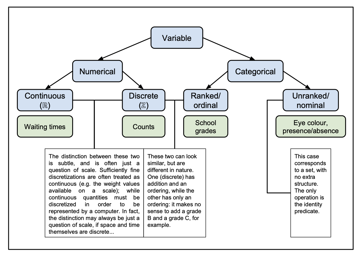
Figure 1.1: Diagram of the different types of variables.
1.4.2 Poisson Distribution
The Poisson distribution is a simple distribution for count data, for which integer values \(x \in \{0,1,2,...\}\) and parameter \(\lambda>0\) has the form \[\begin{equation} P(X=x) = \frac{\lambda^x e^{- \lambda}}{x!} \end{equation}\] We notate this \[\begin{equation} X \sim Poi(\lambda) \end{equation}\]
1.4.3 Multinomial Distribution
Assume random variables \(\boldsymbol{Y} = (Y_1,...,Y_k)^T\), such that \(Y_j \in \{0,...,n\}\) and \(\sum_{j=1}^k Y_j = n\). We say that \(\boldsymbol{Y}\) follows a Multinomial distribution with parameters
- \(n>0\), the number of trials
- \(\boldsymbol{\pi} = (\pi_1,...,\pi_k)^T\), the success vector of probabilities such that \(\pi_i \in (0,1)\) and \(\sum_{j=1}^k \pi_j = 1\)
if \[\begin{equation} P(\boldsymbol{Y} = \boldsymbol{y}) = \frac{n!}{y_1!...y_k!} \pi_1^{y_1}...\pi_k^{y_k} \mathcal{I}_{\boldsymbol{y} \in \mathcal{Y}} \end{equation}\] where
- \(\boldsymbol{y} = (y_1,...,y_k)^T\)
- \(\mathcal{Y} = \{\boldsymbol{y} \in \{0,...,n\}^k | \sum_{j=1}^k y_j = n\}\)
We notate this as \[\begin{equation} \boldsymbol{Y} \sim Mult(n, \boldsymbol{\pi}) \end{equation}\]
1.4.3.1 Mean and Variance
The expectation is7 \[\begin{align} {\mathrm E}[Y_j] & = n \pi_j, \qquad j = 1,...,k \\ {\mathrm E}[\boldsymbol{Y}] & = n \boldsymbol{\pi} \end{align}\]
The covariance structure is8 \[\begin{align} {\mathrm{Var}}[Y_j] & = n \pi_j (1-\pi_j) \\ {\mathrm{Cov}}[Y_j,Y_{j'}] & = -n \pi_j \pi_{j'} \qquad (j \neq j') \\ {\mathrm{Var}}[\boldsymbol{Y}] & = n( \textrm{diag} (\boldsymbol{\pi}) - \boldsymbol{\pi} \boldsymbol{\pi}^T ) \end{align}\]
1.4.3.2 Collapsing Categories
Collapsing categories of a Multinomial distribution leads to another Multinomial distribution with fewer categories.
For example, take a multinomial distribution with seven categories \(A_1,...,A_7\) such that
\[\begin{equation}
(N_1,...,N_7) \sim Mult(n;(\pi_1,...,\pi_7))
\end{equation}\]
Now, if we combine the categories as follows;
\(B_1 = \{A_1, A_2, A_3, A_4\}\),
\(B_2 = A_5\), and
\(B_3 = \{A_6, A_7\}\), then
\((Y_1, Y_2, Y_3) = (N_1 + N_2 + N_3 + N_4, N_5, N_6 + N_7)\) follow a multinomial distribution
\[\begin{equation}
(Y_1, Y_2, Y_3) \sim Mult(n; (\pi_1^* , \pi_2^* , \pi_3^*))
\end{equation}\]
with \((\pi_1^* , \pi_2^* , \pi_3^*) = (\pi_1 + \pi_2 + \pi_3 + \pi_4, \pi_5, \pi_6 + \pi_7)\).
1.4.3.3 Distribution of Outcome Subsets
Suppose we are interested in the first \(Q<K\) outcomes9, then \[\begin{equation} (N_1,...,N_Q) \sim Mult(n_Q; (\pi_1/\pi_Q ,...,\pi_q/\pi_Q)) \end{equation}\] where \(n_Q = \sum_{i=1}^q n_i\) and \(\pi_Q = \sum_{i=1}^q \pi_i\).
1.4.3.4 Poisson and Multinomial Distributions
The conditional distribution of independent Poisson variables \(X_1,...,X_K\) given that their sum \(\sum_{k=1}^K X_k = n\) is \[\begin{eqnarray} P( (X_1=n_1,...,X_K=n_K) | \sum_{k=1}^K X_k = n ) & = & \frac{P(X_1=n_1,...,X_K=n_K)}{P(\sum_{k=1}^K X_K = n)} \\ & = & \frac{\prod_{k=1}^K (e^{-\lambda_k} \lambda_k^{n_k})/n_k!}{(e^{-\lambda} \lambda^n)/n!} \end{eqnarray}\] where we have used the result of Section 1.4.2.2 in the denominator and defined \(\lambda = \sum_{k=1}^K \lambda_k\). Since \(\sum_{k=1}^K n_k = n\), and \(\prod_{k=1}^K e^{- \lambda_k} = e^{- \sum_{k=1}^K \lambda_k} = e^{-\lambda}\), we have that \[\begin{equation} P( (X_1=n_1,...,X_K=n_K) | \sum_{k=1}^K X_k = n ) = \frac{n!}{n_1!n_2!...n_K!} \prod_{k=1}^K \left( \frac{\lambda_k}{\lambda} \right)^{n_k} \end{equation}\] which is \(Mult(n,\boldsymbol{\pi})\), with \(\pi_k = \lambda_k/\lambda\), \(1 \leq k \leq K\), being the components of \(\boldsymbol{\pi}\).
1.4.4 Hypergeometric Distribution
Consider a population of \(N\) items, with \(M\) of them being of a particular type \(\mathcal{A}\) of interest.
If a sample of size \(q\) is selected from this population, then the number \(X\) of type \(\mathcal{A}\) items in the sample is modelled by the hypergeometric distribution, notated
\[\begin{equation}
X \sim \mathcal{H} g (N,M,q)
\end{equation}\]
according to which10
\[\begin{equation}
P(X=x) = \frac{\binom{M}{x}\binom{N-M}{q-x}}{\binom{N}{q}} \qquad \max(0,q-(N-M)) \leq x \leq \min(q,M)
\end{equation}\]
1.4.5 Chi-Squared Distribution
The central chi-squared distribution with \(n\) degrees of freedom is defined as the sum of squares of \(n\) independent standard normal variables \(Z_i \sim \mathcal{N}(0,1), i = 1,...,n\). It is denoted by \[\begin{equation} X^2 = \sum_{i=1}^n Z_i^2 \sim \chi^2(n) \end{equation}\]
1.4.5.1 Mean and Variance
If \(X^2\) has the distribution \(\chi^2(n)\), then11 \[\begin{align} {\mathrm E}[X^2] & = n \\ {\mathrm{Var}}[X^2] & = 2n \end{align}\]
1.4.5.2 Sum of Chi-Squareds
If \(X_1^2,...,X_m^2\) are \(m\) independent variables with chi-squared distributions \(X_i^2 \sim \chi^2(n_i)\), then12 \[\begin{equation} \sum_{i=1}^m X_i^2 = \chi^2(\sum_{i=1}^m n_i ) \end{equation}\]
1.4.6 Central Limit Theorem
The Central Limit Theorem (CLT) tells us that the average \(\bar{X}\) of a sum of \(n\) i.i.d. variables with mean \(\mu\) and variance \(\sigma^2\) will be distributed as: \[\begin{equation} \bar{X} \sim \mathcal{N}(\mu, \frac{\sigma^2}{n}) \end{equation}\] as \(n \rightarrow \infty\).
In higher dimensions, the CLT states that the average \(\bar{\boldsymbol{X}}\) of \(n\) i.i.d. variables with mean vector \(\boldsymbol{\mu}\) and variance matrix \(\Sigma\) will be such that: \[\begin{equation} \sqrt{n} ( \bar{\boldsymbol{X}} - \boldsymbol{\mu} ) \sim {\mathcal N}( \boldsymbol{0}, \Sigma ) \end{equation}\] as \(n \rightarrow \infty\).
1.4.7 Lagrange Multipliers
We here review the essence of optimisation using Lagrange multipliers. For further detail, see the relevant notes from AMVII.
We want to optimise a function \(f(\boldsymbol{x}) \in {\mathbb R}\), with \(\boldsymbol{x} \in {\mathbb R}^t\), subject to the vector constraint \(\boldsymbol{g}(\boldsymbol{x}) = \boldsymbol{0}\), with \(\boldsymbol{g}(\boldsymbol{x}) \in {\mathbb R}^s\) being \(s\) component constraints.
We construct a function, called the Lagrange function, given by \[\begin{equation} \mathcal{L}(\boldsymbol{x}, \boldsymbol{\lambda}) = f(\boldsymbol{x}) + \lambda_1 g_1(\boldsymbol{x}) + ... + \lambda_s g_s(\boldsymbol{x}) \end{equation}\] where \(\boldsymbol{g}(\boldsymbol{x}) = ( g_1(\boldsymbol{x}), ..., g_s(\boldsymbol{x}) )\) and \(\boldsymbol{\lambda} = (\lambda_1,...,\lambda_s)^T\) represents a vector of Lagrange multipliers.
Note that the Lagrange function can also be constructed by substracting the constraint functions, that is \[\begin{equation} \mathcal{L}(\boldsymbol{x}, \boldsymbol{\lambda}) = f(\boldsymbol{x}) - ( \lambda_1 g_1(\boldsymbol{x}) + ... + \lambda_s g_s(\boldsymbol{x}) ) \end{equation}\] It doesn’t make any difference to solving the problem, as the solutions for the local optima of the parameters of interest \(\boldsymbol{x}\) will be the same13.
- To find the points of local optimisation of \(f(\boldsymbol{x})\) subject to the equality constraints, we find the stationary points of Lagrange function \(\mathcal{L}(\boldsymbol{x}, \boldsymbol{\lambda})\), that is, we solve the following system of equations: \[\begin{eqnarray} \frac{\partial \mathcal{L}}{\partial x_i} & = & 0 \qquad i = 1,...,t \\ \frac{\partial \mathcal{L}}{\partial \lambda_j} & = & 0 \qquad j = 1,...,s \end{eqnarray}\]
1.5 Acronyms
A reference to some of the acronyms used during the course:
- AIC - Aikaike Information Criterion
- ANOVA - Analysis of Variance
- BIC - Bayesian Information Criterion
- BPD - Bronchopulmonary dysplasia (specific to
bpdexample dataset) - CDF - Cumulative Distribution Function
- CI - Confidence Interval
- CLT - Central Limit Theorem
- DSSC - Data Science and Statistical Computing
- EDF - Exponential Dispersion Family
- EF - Exponential Family
- GLM - Generalised Linear Model
- GLR - Generalised Likelihood Ratio
- HLLM - Hierarchical Log Linear Model
- i.i.d. - independent and identically distributed
- IWLS - Iterative Weighted Least Squares
- LLM - Log Linear Model
- LR - Likelihood Ratio
- ML - Maximum Likelihood
- MLE - Maximum Likelihood Estimator/Estimation
- PDF - Probability Density Function
- RSS - Residual Sum of Squares
- SSE - Sum of Squares of the Error (equivalent to RSS)
- SSR - Sum of Squares of the Regression
- SST - Sum of Squares Total
1.6 Key References
You are encouraged to read about widely, expanding your knowledge beyond the notes contained here.
Useful references for the first half of this course are the following:
Kateri (2014) - Contingency Table Analysis - Methods and Implementation Using R, by Maria Kateri.
Tutz (2012) - Regression for Categorical Data, by Gerhard Tutz.
Agresti (2019) - An Introduction to Categorical Data Analysis, - by Alan Agresti.
Bilder and Loughin (2015) - Analysis of Categorical Data with R, - by Christopher Bilder and Thomas Loughin.
Faraway (2016) - Extending The Linear Model with R - Generalized Linear, Mixed Effects and Nonparametric Regression Models, by Julian Faraway.
You can explore the references contained within these books (and these lecture notes) for further information, and take yourselves on a journey of exploration.
References
We will here assume that \(\theta\) is a scalar parameter↩︎
See the corresponding lecture notes (Theorem 6.3) for the mathematical exposition of this theorem.↩︎
For the purposes of this course, we will use this theorem without proof. A sketch of the proof was outlined in Statistical Inference II. Anyone who is interested in Wilks’ original paper on the theorem can consult Wilks (1938).↩︎
\(\mathcal{I}_T\) is the indicator function taking value 1 if \(T\) holds and 0 otherwise.↩︎
Terminology: The term fitted value is typically used for an estimate of a piece of data used to fit the model, and predicted value is typically used for an estimate of a piece of data not used to fit the model, but they are mathematically the same.↩︎
Recall that \(Y_0\) and \(\hat{Y}_0\) are independent since \(\hat{Y}_0\) is a linear combination of \(y_1,...,y_n\).↩︎
Q1-3 concerns proving the results stated in this section.↩︎
Note that \(\textrm{diag}(\boldsymbol{\pi})\) is the \(k \times k\) diagonal matrix with diagonal elements taking the values of the vector \(\boldsymbol{\pi}\).↩︎
or indeed, any collection of \(Q<K\) outcomes.↩︎
Note that this is a counting problem. The denominator is the number of ways to sample \(q\) items from the total \(N\), and the numerator is the number of ways in which to sample \(x\) of the \(M\) type \(\mathcal{A}\) objects, and \(q-x\) of the \(N-M\) non-type \(\mathcal{A}\) objects.↩︎
Q1-3c involves proving that the results of this section hold.↩︎
Q1-3b involves showing that the result of this section holds.↩︎
Indeed, I use the subtraction convention later on.↩︎