Chapter 4 Log-Linear Models
- We have dealt with inter-relationships among and between several categorical variables in Sections 2 and 3.
Log-Linear Models (LLMs) describe the way the involved categorical variables and their association (if appropriate/significant) influence the count in each of the cells of the cross-classification table of these variables.
They are appropriate when there is no clear distinction between response and explanatory variables (this is in contrast to GLMs (later…)).
So, how precisely are they formed…?
4.1 LLMs for Two-Way Tables
4.1.1 Model of Independence
Independence between classification variables \(X\) and \(Y\) can equivalently be expressed in terms of the expected-under-independence cell frequencies \(E_{ij}\) in a log-linear model form as \[\begin{equation} \log E_{ij} = \lambda + \lambda_i^X + \lambda_j^Y \qquad \forall i,j \tag{4.1} \end{equation}\] where
\(\lambda_i^X\) corresponds to the effect of the \(i^\textrm{th}\) level of \(X\), and
\(\lambda_j^Y\) corresponds to the effect of the \(j^\textrm{th}\) level of \(Y\)
What about \(\lambda\)? Well that depends on the choice of constraints used (Section 4.1.1.4). The precise interpretation of \(\lambda_i^X\) and \(\lambda_j^Y\) also depends on the choice of constraints used.
4.1.1.1 Interpretation via Odds
Interpretation is carried out in terms of odds. For given column category \(j\), under the model given by Equation (4.1), the odds of being in row \(i_1\) instead of row \(i_2\), for \(i_1, i_2 \in \{1,...,I\}, i_1 \neq i_2\), are \[\begin{equation} \frac{E_{i_1j}}{E_{i_2j}} = \frac{\exp(\lambda + \lambda_{i_1}^X + \lambda_j^Y)}{\exp(\lambda + \lambda_{i_2}^X + \lambda_j^Y)} = \exp(\lambda_{i_1}^X - \lambda_{i_2}^X) \qquad \forall j \tag{4.2} \end{equation}\] which shows that being in row \(i_1\) instead of \(i_2\) is determined only by the distance of the corresponding row main effect values, and hence independent of \(j\). Note that Equation (4.2) also implies that \[\begin{equation} \frac{P(X = i_1|Y= j)}{P(X = i_2|Y= j)} = \exp(\lambda_{i_1}^X - \lambda_{i_2}^X) \qquad \forall j \end{equation}\]
Similarly for columns \(j_1\) and \(j_2\) such that \(j_1, j_2 \in \{1,...,J\}, j_1 \neq j_2\), we have \[\begin{equation} \frac{E_{ij_1}}{E_{ij_2}} = \exp(\lambda_{j_1}^Y - \lambda_{j_2}^Y) \qquad \forall i \end{equation}\] hence independent of \(i\).
4.1.1.2 Odds Ratios
- Local odds ratios in this case are given by \[\begin{equation} r_{ij}^L = \frac{E_{ij}/E_{i+1,j}}{E_{i,j+1}/E_{i+1,j+1}} = \frac{\exp(\lambda_{i}^X - \lambda_{i+1}^X)}{\exp(\lambda_{i}^X - \lambda_{i+1}^X)} = 1 \qquad i = 1,...,I-1 \quad j = 1,...,J-1 \end{equation}\] as expected.
4.1.1.3 Non-Identifiability Issues
We observe that the model given by Equation (4.1) has \(1 + I + J\) parameters to be learned.
However, under a Poisson sampling scheme, there should be \(1 + (I-1) + (J-1)\) free parameters, because
- \(n_{++}\) is not fixed, hence we have to learn it (1 parameter),
- the set of marginal sums \(n_{i+}\) must themselves sum to \(n_{++}\), hence \((I-1)\) parameters,
- the set of marginal sums \(n_{+j}\) must themselves sum to \(n_{++}\), hence \((J-1)\) parameters.
4.1.1.4 Identifiability Constraints
To fix the non-identifiability issues, we impose a number of constraints equal to the difference between the number of free parameters of the unconstrained model and the number it should have.
For the two-way independence model, this is: \[(1 + I + J) - (1 + (I-1) + (J-1)) = 2\]
We discuss two popular choices.
4.1.1.4.1 Zero-Sum Constraints
\[\begin{equation} \sum_{i=1}^I \lambda_i^X = \sum_{j=1}^J \lambda_j^Y = 0 \end{equation}\]
Then \(\lambda_i^X\) and \(\lambda_j^Y\) account for deviations that \(X\) and \(Y\) have from the overall mean (\(\lambda\)).
4.1.1.4.2 Corner Point Constraints
\[\begin{equation} \lambda_I^X = \lambda_J^Y = 0 \end{equation}\] where \(I\) and \(J\) are called reference levels for variables \(X,Y\).
Then \(\lambda_i^X, \, i = 1,...,I-1\) and \(\lambda_j^Y, \, j = 1,...,J-1\) account for deviations from the reference levels \(I\) and \(J\).
Of course, any other level could serve as reference levels instead. For example, \[\begin{equation} \lambda_1^X = \lambda_1^Y = 0 \end{equation}\] is a common choice too.
4.1.1.4.3 Interpretations of \(\lambda\)
- Different identifiability constraints lead to different interpretation for the \(\lambda\)’s, but to the same inference.
4.1.1.4.3.1 Example
For a \(2 \times 2\) contingency table, we have
with zero-sum constraints (\(\lambda_1^X + \lambda_2^X = \lambda_1^Y + \lambda_2^Y = 0\)), that \[\begin{equation} \frac{\pi_{2|i}}{\pi_{1|i}} = \exp(-2 \lambda_1^Y) \end{equation}\]
or with corner point constraints (\(\lambda_2^X = \lambda_2^Y = 0\)), that \[\begin{equation} \frac{\pi_{2|i}}{\pi_{1|i}} = \exp(- \lambda_1^Y) \end{equation}\]
4.1.2 The Saturated Model
If \(X, Y\) are not independent, then we add an \(XY\)-interaction term to the LLM. \[\begin{equation} \log E_{ij} = \lambda + \lambda_i^X + \lambda_j^Y + \lambda_{ij}^{XY} \qquad \forall i,j \tag{4.3} \end{equation}\]
4.1.2.1 Log Odds Ratio
The local odds ratios are directly derived from the interaction parameters, since \[\begin{equation} \log r_{ij}^L = \lambda_{ij}^{XY} + \lambda_{i+1,j+1}^{XY} - \lambda_{i+1,j}^{XY} - \lambda_{i,j+1}^{XY} \qquad i = 1,...,I-1, \, j = 1,...,J-1 \tag{4.4} \end{equation}\]
4.1.2.2 Constraints
4.1.2.3 Free Parameters
The number of free parameters (under Poisson sampling) is thus \[\begin{equation} d = 1 + (I-1) + (J-1) + (I-1)(J-1) = IJ \end{equation}\] as it should, corresponding to the number of cells in the table.
Remark: Under multinomial sampling, since \(n_{++}\) is fixed, there should be \(IJ-1\) parameters. This is fixed by removing \(\lambda\) as a parameter.
4.1.3 Interpretation of \(\lambda\)
From Equation (4.3), assuming the zero-sum constraints as given by Equation (4.5), we have that45 \[\begin{eqnarray} \lambda & = & \frac{1}{IJ} \sum_{i,j} \log E_{ij} \tag{4.6} \\ \lambda_i^X & = & \frac{1}{J} \sum_{j} \log E_{ij} - \lambda \qquad i = 1,...,I \tag{4.7} \\ \lambda_j^Y & = & \frac{1}{I} \sum_{i} \log E_{ij} - \lambda \qquad j = 1,...,J \tag{4.8} \\ \lambda_{ij}^{XY} & = & \log E_{ij} - \lambda - \lambda_i^X - \lambda_j^Y \qquad i = 1,...,I, j = 1,...,J \tag{4.9} \end{eqnarray}\]
Hence,
\(\lambda\) represents the mean in terms of being the mean log expected count value across all cells in the table.
\(\lambda_i^X\) represents the effect of the \(i^{th}\) level of \(X\) as the difference between the average log expected count value across the levels of \(Y\) conditional on \(X=i\), and the overall average log expected count value across all cells in the table46.
\(\lambda_{ij}^{XY}\) represents the joint effect of the \(i^{th}\) level of \(X\) and the \(j^{th}\) level of \(Y\) as the difference between the log expected cell count for cell \((i,j)\), and the sum of the marginal contributions attributed to \(\lambda\), \(\lambda_i^X\) and \(\lambda_j^Y\) discussed above.
4.1.4 Inference and Fit
The likelihood function (\(Poi(E_{ij})\)-distributed for each cell \((i,j)\)): \[\begin{equation} L = \prod_{i,j} \frac{e^{-E_{ij}} E_{ij}^{n_{ij}}}{n_{ij}!} \end{equation}\] so that \[\begin{eqnarray} l & = & \sum_{i,j} (-E_{ij} + n_{ij} \log E_{ij} - \log n_{ij}!) \\ & \propto & \sum_{i,j} (n_{ij} \log E_{ij} - e^{\log E_{ij}}) \tag{4.10} \end{eqnarray}\] as an expression of \(\log E_{ij}\).
Substituting \(\log E_{ij}\) using the relevant expression (e.g. from Equation (4.1) for the independence model or Equation (4.3) for the saturated model) will make this an expression of the LLM \(\lambda\) parameters.
We now proceed for the independence model specifically.
4.1.4.1 Inference and Fit for Independence Model under Zero-Sum Constraints
Given model \([X,Y]\), we have \[\begin{eqnarray} \pi_{ij} & = & \pi_{i+} \pi_{+j} \nonumber \\ \implies E_{ij} & = & \frac{E_{i+}E_{+j}}{n_{++}} \tag{4.11} \end{eqnarray}\] since \(E_{ij} = n_{++} \pi_{ij}\), \(E_{i+} = n_{++} \pi_{i+}\), etc.
Hence we have that \[\begin{equation} \hat{E}_{ij} = \frac{\hat{E}_{i+}\hat{E}_{+j}}{n_{++}} \end{equation}\] where \(\hat{E}_{ij} = n_{++} \hat{\pi}_{ij}\), \(\hat{E}_{i+} = n_{++} \hat{\pi}_{i+}\) etc.
In Section 2.4.3.2, we used the method of Lagrange multipliers to find MLEs \(\hat{\pi}_{i+}\) and \(\hat{\pi}_{+j}\) using appropriate independence constraints. These can then be used to yield \(\hat{E}_{i+}\) and \(\hat{E}_{+j}\).
Alternatively, however, we could also use the method of Lagrange multipliers for \(\lambda\) on the log-likelihood of the LLM expression (such as given by Equation (4.10)) to elicit MLEs \(\hat{E}_{i+} \equiv E_{i+}(\hat{\boldsymbol{\lambda}})\) and \(\hat{E}_{+j} \equiv E_{+j}(\hat{\boldsymbol{\lambda}})\)47.
Either way, we find that \[\begin{equation} \hat{E}_{i+} = n_{i+} \qquad \hat{E}_{+j} = n_{+j} \end{equation}\] so that \[\begin{equation} \hat{E}_{ij} = \frac{\hat{E}_{i+}\hat{E}_{+j}}{n_{++}} = \frac{n_{i+}n_{+j}}{n_{++}} \tag{4.12} \end{equation}\]We can then substitute these estimates \(\hat{E}_{ij}\) into Equations (4.6) - (4.8)48 to obtain MLEs for the LLM parameters as given by:49 50 \[\begin{eqnarray} \hat{\lambda} & = & \frac{1}{I} \sum_s \log n_{s+} + \frac{1}{J} \sum_{t} \log n_{+t} - \log n_{++} \tag{4.13} \\ \hat{\lambda}_{i+} & = & \log n_{i+} - \frac{1}{I} \sum_s \log n_{s+} \qquad i = 1,...,I \tag{4.14} \\ \hat{\lambda}_{+j} & = & \log n_{+j} - \frac{1}{J} \sum_t \log n_{+t} \qquad j = 1,...,J \tag{4.15} \end{eqnarray}\]
4.2 LLMs for Three-Way Tables
- Consider a three-way contingency table, cross-classifying the variables \(X\), \(Y\) and \(Z\).
4.2.1 Mutual Independence
- Denoted \([X,Y,Z]\), this is given as \[\begin{equation} \log E_{ijk} = \lambda + \lambda_i^X + \lambda_j^Y + \lambda_k^Z \qquad \forall i,j,k \end{equation}\] with either zero-sum constraints: \[\begin{equation} \sum_{i=1}^I \lambda_i^X = \sum_{j=1}^J \lambda_j^Y = \sum_{k=1}^K \lambda_k^Z = 0 \tag{4.16} \end{equation}\] or corner point constraints: \[\begin{equation} \lambda_I^X = \lambda_J^Y = \lambda_K^Z = 0 \tag{4.17} \end{equation}\] so that the number of free parameters is \[\begin{equation} d = 1 + (I-1) + (J-1) + (K-1) = I + J + K - 2 \end{equation}\]
4.2.2 Joint Independence
Joint independence of \(Y\) from \(X\) and \(Z\) (denoted \([Y,XZ]\)) corresponds to the following LLM: \[\begin{equation} \log E_{ijk} = \lambda + \lambda_i^X + \lambda_j^Y + \lambda_k^Z + \lambda_{ik}^{XZ} \qquad \forall i,j,k \end{equation}\] either satisfying the zero-sum constraints given by Equation (4.16) in addition to \[\begin{equation} \sum_{i=1}^I \lambda_{ik}^{XZ} = \sum_{k=1}^K \lambda_{ik}^{XZ} = 0 \end{equation}\] for all possible values of the non-marginal subscript, or satisfying the cornerpoint constraints given by Equation (4.17) in addition to \[\begin{equation} \lambda_{Ik}^{XZ} = \lambda_{iK}^{XZ} = 0 \end{equation}\] for all possible values of the non-conditional subscript.
As a result, the number of free parameters for this model is given by \[\begin{equation} d = 1 + (I-1) + (J-1) + (K-1) + (I-1)(K-1) = IK + J - 1 \end{equation}\]
4.2.3 Further LLMs
Hopefully you can see that LLMs corresponding to the types of independence discussed in Sections 3.3.1 to 3.3.6 are also possible, as well as a three-way saturated model for the situation where all three parameters are all jointly associated with each other.
4.2.3.1 Homogeneous Associations Model
The homogeneous associations model is \[\begin{equation} \log E_{ijk} = \lambda + \lambda_i^X + \lambda_j^Y + \lambda_k^Z + \lambda_{ij}^{XY} + \lambda_{ik}^{XZ} + \lambda_{jk}^{YZ} \qquad \forall i,j,k \end{equation}\] with zero-sum constraints51 given by \[\begin{equation} \sum_{i=1}^I \lambda_i^X = \sum_{j=1}^J \lambda_j^Y = \sum_{k=1}^K \lambda_k^Z = \sum_{i=1}^I \lambda_{ij}^{XY} = \sum_{j=1}^J \lambda_{ij}^{XY} = \sum_{i=1}^I \lambda_{ik}^{XZ} = \sum_{k=1}^K \lambda_{ik}^{XZ} = \sum_{j=1}^J \lambda_{jk}^{YZ} = \sum_{k=1}^K \lambda_{jk}^{YZ} = 0 \tag{4.18} \end{equation}\] with the two-factor constraints holding for all values of the non-marginalised subscript.
4.2.3.2 The Saturated Model
The saturated model is \[\begin{equation} \log E_{ijk} = \lambda + \lambda_i^X + \lambda_j^Y + \lambda_k^Z + \lambda_{ij}^{XY} + \lambda_{ik}^{XZ} + \lambda_{jk}^{YZ} + \lambda_{ijk}^{XYZ} \qquad \forall i,j,k \end{equation}\] with zero-sum constraints52 as given by Equation (4.18) in addition to \[\begin{equation} \sum_{i=1}^I \lambda_{ijk}^{XYZ} = \sum_{j=1}^J \lambda_{ijk}^{XYZ} = \sum_{k=1}^K \lambda_{ijk}^{XYZ} = 0 \end{equation}\] each holding for all pairs of values of the non-marginalised subscripts, resulting in \[\begin{eqnarray} d & = & 1 + (I-1) + (J-1) + (K-1) \\ & & \, + (I-1)(J-1) + (I-1)(K-1) + (J-1)(K-1) \\ & & \, + (I-1)(J-1)(K-1) = IJK \end{eqnarray}\] free parameters.
4.3 Hierarchical LLMs for Multiway Tables
LLMs can be defined analogously for multiway tables of \(q>3\) categorical variables.
LLMs for multiway tables include higher-order interactions, up to order \(q\).
The number of possible models increases with the dimension of the table, involving the procedure of deciding which one is appropriate for describing the underlying structure of association.
In order to impose a structure on model building, especially helpful in model selection, log-linear modelling is usually restricted to the family of Hierarchical Log-Linear Models (HLLMs).
Hierarchical here means that if an interaction term of \(b\) variables is included in the model, then all the marginal terms, corresponding to lower-level interactions of any subset of these \(b\) variables, will also be included.
4.3.1 Example: \([XYW,ZW]\)
In a four-way table cross-classifying variables \(X, Y, Z\) and \(W\), how could we understand and explain that variable \(X\) does not interact with \(Y\) (absence of the \(\lambda_{XY}\) term from the model) but it interacts simultaneously with \(Y\) and \(W\) (model includes the \(\lambda_{ijl}^{XYW}\) term)?
Therefore, if \(\lambda_{ijl}^{XYW}\) is included, so too must \(\lambda_{ij}^{XY}\), \(\lambda_{il}^{XW}\) and \(\lambda_{jl}^{YW}\), and by extension or directly, \(\lambda_{i}^{X}\), \(\lambda_{j}^{Y}\) and \(\lambda_{l}^{W}\) must be included as well.
\([XYW,ZW]\) therefore implies the following model \[\begin{equation} \log E_{ijkl} = \lambda + \lambda_i^X + \lambda_j^Y + \lambda_k^Z + \lambda_l^W + \lambda_{ij}^{XY} + \lambda_{il}^{XW} + \lambda_{jl}^{YW} + \lambda_{kl}^{ZW} + \lambda_{ijl}^{XYW} \qquad \forall i,j,k,l \end{equation}\]
This model implies that \(XY\) are jointly independent of \(Z\) conditional on \(W\), since the two-factor interaction terms \(XZ\) and \(YZ\) are missing. Another way to see this is that no term involves both \(Z\) and ‘\(X\) or \(Y\)’, so if \(W\) is fixed at level \(l\), then \(Z\) and \(XY\) affect \(\log E_{ijkl}\) independently. Note, however, that the model structure does not imply that \(Z\) and \(XY\) are jointly independent if we marginalise over \(W\).
4.3.2 Example: \([XYW,Z]\)
- If the model of interest is notated \([XYW,Z]\) (that is, \(XYW\) are jointly independent of \(Z\)), then the model is given by \[\begin{equation} \log E_{ijkl} = \lambda + \lambda_i^X + \lambda_j^Y + \lambda_k^Z + \lambda_l^W + \lambda_{ij}^{XY} + \lambda_{il}^{XW} + \lambda_{jl}^{YW} + \lambda_{ijl}^{XYW} \qquad \forall i,j,k,l \end{equation}\]
4.3.3 Example: \([X_1X_2,X_1X_5,X_3X_4X_5,X_5X_6X_7]\)
\([X_1X_2,X_1X_5,X_3X_4X_5,X_5X_6X_7]\) implies the following model \[\begin{eqnarray} \log E_{i_1...i_7} & = & \lambda + \sum_{q=1}^7 \lambda_{i_q}^{X_q} \nonumber \\ && + \lambda_{i_1i_2}^{X_1X_2} + \lambda_{i_1i_5}^{X_1X_5} + \lambda_{i_3i_4}^{X_3X_4} + \lambda_{i_3i_5}^{X_3X_5} + \lambda_{i_4i_5}^{X_4X_5} + \lambda_{i_5i_6}^{X_5X_6} + \lambda_{i_5i_7}^{X_5X_7} + \lambda_{i_6i_7}^{X_6X_7} \nonumber \\ && + \lambda_{i_3i_4i_5}^{X_3X_4X_5} + \lambda_{i_5i_6i_7}^{X_5X_6X_7} \qquad \forall i_1,i_2,i_3,i_4,i_5,i_6,i_7 \tag{4.19} \end{eqnarray}\]
We can see that variable pairs \((X_1,X_2)\), \((X_3,X_4)\) and \((X_6,X_7)\) are mutually independent conditional on \(X_5\).
4.3.4 Notation
Notation can get ridiculous here…
We can also write the model (4.19) as \[\begin{equation} \log E_{i_1...i_7} = \lambda + \sum_{\mathcal{I} \in \mathcal{J}} \lambda_{\mathcal{I}}^{\mathcal{X}} \end{equation}\] where \(\mathcal{I}\) corresponds to the levels of a combination of variables \(\mathcal{X}\) included in a particular model term, and \(\mathcal{J}\) corresponds to the set of those combinations which make up the terms of the whole model.
Using this notation, for the model given by Equation (4.19), we have \[\begin{eqnarray} \mathcal{J} = \{\mathcal{I}\} & = & \{ i_1, i_2, i_3, i_4, i_5, i_6, i_7, \nonumber \\ && (i_1, i_2), (i_1, i_5), (i_3, i_4), (i_3, i_5), (i_4, i_5), (i_5, i_6), (i_5, i_7), (i_6, i_7), \nonumber \\ && (i_3, i_4, i_5), (i_5, i_6, i_7) \} \end{eqnarray}\] corresponding to the sets of variables \[\begin{eqnarray} \{\mathcal{X}\} & = & \{ X_1, X_2, X_3, X_4, X_5, X_6, X_7, \nonumber \\ && (X_1, X_2), (X_1, X_5), (X_3, X_4), (X_3, X_5), (X_4, X_5), (X_5, X_6), (X_5, X_7), (X_6, X_7), \nonumber \\ && (X_3, X_4, X_5), (X_5, X_6, X_7) \} \end{eqnarray}\]
4.4 MLE for LLMs
This is the general five-step process of obtaining MLEs for the LLM \(\lambda\) parameters. Some of these involve quite some work in themselves.53
1. Write down log-likelihood expression.
- Similar to Section 4.1.4 for the two-way LLM, assuming a \(Poi(E_{i_1...i_q})\) distribution for each cell \((i_1,...,i_q)\), the general log-likelihood is \[\begin{equation} l(\boldsymbol{\lambda}) \propto \sum_{i_1,...,i_q} n_{i_1...i_q} \log(E_{i_1...i_q}) - E_{i_1...i_q} = \sum_{i_1,...,i_q} n_{i_1...i_q} \log(E_{i_1...i_q}) - e^{\log(E_{i_1...i_q})} \end{equation}\] where \(E_{i_1...i_q} \equiv E_{i_1...i_q}(\boldsymbol{\lambda})\) can be viewed as a function of \(\boldsymbol{\lambda}\) which is defined by the LLM expression of interest.
2. \(E_{i_1...i_q}\) only depend on \(E_{\mathcal{I}}\).
- We can use knowledge of the model format/dependency structure to express \(E_{i_1...i_q}\) in terms of \(E_{\mathcal{I}}\). In other words, we only require \(E_{\mathcal{I}}\) corresponding to \(\mathcal{I} \in \mathcal{J}\), from which \(E_{i_1...i_q}, \, \forall i_1,...,i_q\), can be obtained given the dependency structure corresponding to \(\mathcal{J}\). It may be possible to express this dependency in an analytic form (such as Equation (4.11) for model \([X,Y]\), or Equation (4.21) below for model \([Y, XZ]\)), or it may be that a tractable expression is not available, in which case numerical methods such as Newton-Raphson or Iterative Proportional Fitting must be used, as discussed in Section 3.3.654). See Section 4.4.1 for examples.
3. Use Lagrange multipliers to elicit required \(\hat{E}_{\mathcal{I}} \equiv E_{\mathcal{I}}(\hat{\lambda})\)-terms.
We do this either
through first eliciting required \(\hat{\pi}\)-terms, or
for \(\hat{\lambda}\) on the log-likelihood of LLM expression, with corresponding constraints.
Either way, we find that \[\begin{equation} \hat{E}_{\mathcal{I}} = n_{\mathcal{I}} \end{equation}\] for all \(\mathcal{I} \in \mathcal{J}\), where \(n_{\mathcal{I}}\) corresponds to the marginal sums over all levels of the variables not represented in the set \(\mathcal{I}\).
4. Obtain MLEs for \(\hat{E}_{i_1...i_q} \equiv E_{i_1...i_q}(\hat{\boldsymbol{\lambda}})\) terms.
We do this by either using the expression from (2.) if obtained, or by appropriate numerical approximation method55 if no analytical expression exists.
Either way, MLEs for the remaining \(\hat{E}_{i_1,...,i_q} \equiv E_{i_1,...,i_q}(\hat{\boldsymbol{\lambda}})\) terms, \(\forall i_1,...,i_q\), only depend on (that is, can be obtained from) the \(\hat{E}_\mathcal{I}\) terms corresponding to those \(\mathcal{I} \in \mathcal{J}\) included in the model (see Section 4.4.1 for examples).
5. Substitute these estimates \(\hat{E}_{i_1...i_q}\) into expressions for \(\boldsymbol{\lambda}\)
The \(\hat{\lambda}\) LLM parameters can then be found by:
first rearranging the equations corresponding to the LLM expressions in terms of the \(\lambda\) parameters (such as for the two-way saturated model in Section 4.1.3); and
then substituting the relevant estimates \(\hat{E}_{i_1...i_q}\) into these expressions for \(\boldsymbol{\lambda}\) (such as for the two-way independence model in Section 4.1.4.1).
4.4.1 Examples of Eliciting \(\hat{E}_{i_1,...,i_q}\)
4.4.1.1 \([Y, XZ]\)
\(E_{ijk}\) only depend on \(E_{+j+}\) and \(E_{i+k}\) as follows \[\begin{equation} E_{ijk} = \frac{E_{+j+}E_{i+k}}{n_{+++}} \tag{4.20} \end{equation}\]
Using Lagrange multipliers, we can show that \(\hat{E}_{+j+} = n_{+j+}\) and \(\hat{E}_{i+k} = n_{i+k}\), so that \[\begin{equation} \hat{E}_{ijk} = \frac{\hat{E}_{+j+}\hat{E}_{i+k}}{n_{+++}} = \frac{n_{+j+}n_{i+k}}{n_{+++}} \tag{4.21} \end{equation}\]
4.4.1.2 \([XY, XZ, YZ]\)
\(\hat{E}_{ijk}\) depends only on \(\hat{E}_{ij} = n_{ij}\), \(\hat{E}_{ik} = n_{ik}\) and \(\hat{E}_{jk} = n_{jk}\). However, this relation cannot be expressed by a tractable expression (hence numerical methods such as Newton-Raphson and Iterative Proportional Fitting must be used, as discussed in Section 3.3.656).
4.5 Model Fit and Selection
4.5.1 Nested Models
Model \(\mathcal{M}_0\) is nested in model \(\mathcal{M}_1\) if and only if \(\mathcal{M}_1\) can be reduced to the simpler \(\mathcal{M}_0\) by assigning specific fixed values (usually \(0\)) to some of the parameters of \(\mathcal{M}_1\).
4.5.1.1 Example
Model \([Y,XZ]\) is nested in model \([XY, XZ]\) since \[\begin{equation} \log E_{ijk} = \lambda + \lambda_i^X + \lambda_j^Y + \lambda_k^Z + \lambda_{ik}^{XZ} \qquad \forall i,j,k \end{equation}\] can be obtained from \[\begin{equation} \log E_{ijk} = \lambda + \lambda_i^X + \lambda_j^Y + \lambda_k^Z + \lambda_{ij}^{XY} + \lambda_{ik}^{XZ} \qquad \forall i,j,k \end{equation}\] by setting \(\lambda_{ij}^{XY} = 0 \qquad \forall i,j\).
4.5.1.2 For Three-Way Tables
Sequences of nested models for three-way tables, from the saturated \([XYZ]\) model to the model of mutual independence \([X,Y,Z]\), are displayed in Figure 4.1.
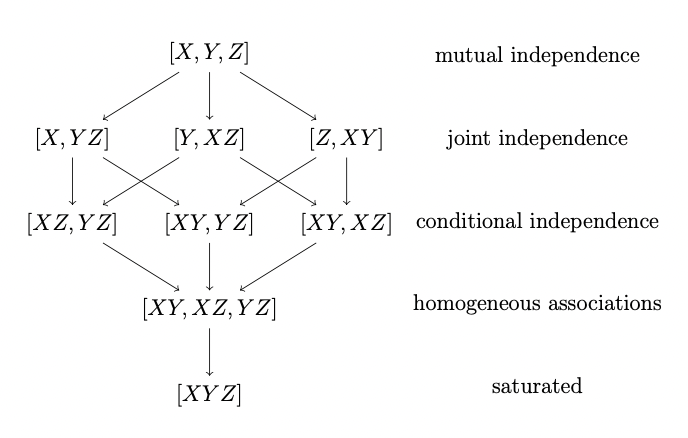
Figure 4.1: Sequences of nested models for three-way tables.
4.5.2 Generalised Goodness-of-Fit Test
We use a Goodness-of-Fit test to test between the two hypotheses: \[\begin{eqnarray} \mathcal{H}_0: & \, \textrm{model (that is, dependency type) } \mathcal{M}_0 \\ \mathcal{H}_1: & \, \textrm{model (that is, dependency type) } \mathcal{M}_1 \end{eqnarray}\] where \(\mathcal{M}_0\) is nested in \(\mathcal{M}_1\).
Using Wilks’ Theorem (Section 1.2.3.4), under \(\mathcal{H}_0\) we have that \[\begin{equation} G^2(\mathcal{M}_0 | \mathcal{M}_1) = 2 \sum_{i_1...i_q} n_{i_1...i_q} \log \biggl( \frac{\hat{E}^{(1)}_{i_1...i_q}}{\hat{E}^{(0)}_{i_1...i_q}} \biggr) \sim \chi^2_{df} \tag{4.22} \end{equation}\] where \(\hat{E}^{(0)}_{i_1...i_q}\) is the MLE of \(E^{(0)}_{i_1...i_q}\) under the model \(\mathcal{M}_0\), \(\hat{E}^{(1)}_{i_1...i_q}\) is the MLE of \(E^{(1)}_{i_1...i_q}\) under the model \(\mathcal{M}_1\), and the degrees of freedom \(df\) are given by \[\begin{equation} df = d_1 - d_0 \end{equation}\] where \(d_0\) is the number of free parameters in model \(\mathcal{M}_0\), and \(d_1\) is the number of free parameters in model \(\mathcal{M}_1\).
Notice that we can show: \[\begin{equation} G^2(\mathcal{M}_0 | \mathcal{M}_1) = G^2(\mathcal{M}_0 | \mathcal{M}_{sat}) - G^2(\mathcal{M}_1 | \mathcal{M}_{sat}) \tag{4.23} \end{equation}\] where \(\mathcal{M}_{sat}\) is the saturated model of dimension \(q\), and \(q\) is the number of variables.
The corresponding rejection area of the GLR test of null hypothesis \(\mathcal{H}_0\) against alternative hypothesis \(\mathcal{H}_1\), at significance level \(\alpha\), is \[\begin{equation} R = \{\boldsymbol{n} : G^2(\mathcal{M}_0|\mathcal{M}_1) \geq \chi^2_{df,\alpha} \} \end{equation}\]
4.5.3 Model Selection
LLM selection consists of a sequential search between hierarchical nested models:
Backwards model selection: start from the saturated model, and at each step remove the least significant term. This term can be found by conditionally testing the significance of each potential term to be removed (ensuring the model is still hierarchical). The process stops and decides for the model for which the next term to be removed leads to a large value of the test statistic given by Equation (4.22).
Forwards model selection: Start from the model of complete independence and at each step add the most significant potential term. This term can be found by conditionally testing the significance of each potential term to be added (ensuring the model is still hierarchical). The process stops and decides for the model for which the next term to be added leads to a small value of the test statistic given by Equation (4.22).
4.5.3.1 Selection Criteria
We need to use some form of criteria to decide between non-nested models in the above stepwise algorithms. We here consider AIC and BIC.
4.5.3.1.1 AIC
- One option is to minimise the Akaike Information Criterion (AIC).
- For model \(\mathcal{M}\), the AIC is given by \[\begin{equation} -2 l_{\mathcal{M}}(\hat{\boldsymbol{\lambda}}) + 2 d_{\mathcal{M}} \tag{4.24} \end{equation}\] where \(l_{\mathcal{M}}(\hat{\boldsymbol{\lambda}})\) is the value of the log-likelihood function at the MLE for \(\boldsymbol{\lambda}\) for the appropriate set of \(\lambda\) parameters corresponding to model \(\mathcal{M}\), and \(d_{\mathcal{M}}\) is the number of free parameters in model \(\mathcal{M}\).
4.5.3.1.2 BIC
- Another option is to minimise the Bayesian Information Criterion (BIC).
- For model \(\mathcal{M}\), the BIC is given by \[\begin{equation} -2 l_{\mathcal{M}}(\hat{\boldsymbol{\lambda}}) + \log(n_{+...+}) d_{\mathcal{M}} \tag{4.25} \end{equation}\] where \(l_{\mathcal{M}}(\hat{\boldsymbol{\lambda}})\) is the value of the log-likelihood function at the MLE for \(\boldsymbol{\lambda}\) for the appropriate set of \(\lambda\) parameters corresponding to model \(\mathcal{M}\), \(d_{\mathcal{M}}\) is the number of free parameters in model \(\mathcal{M}\), and \(n_{+...+}\) is the total number of observations.
4.5.3.1.3 Example: \([Y, XZ]\)
Following Section 4.2.2, assuming Poisson sampling and a model \(\mathcal{M}\) given by \([Y, XZ]\), we have that \[\begin{equation} \hat{E}_{ijk} = \frac{\hat{E}_{i+k} \hat{E}_{+j+}}{n_{+++}} = \frac{n_{i+k} n_{+j+}}{n_{+++}} \end{equation}\] so that \[\begin{eqnarray} l(\hat{\boldsymbol{\lambda}}) & = & \sum_{ijk} ( -\hat{E}_{ijk} + n_{ijk} \log \hat{E}_{ijk} - \log n_{ijk}! ) \\ & = & \sum_{ijk} \biggl( n_{ijk} \log \biggl( \frac{n_{i+k} n_{+j+}}{n_{+++}} \biggr) - \frac{n_{i+k} n_{+j+}}{n_{+++}} - \log n_{ijk}! \biggr) \end{eqnarray}\]
Then we have that \[\begin{eqnarray} AIC(\mathcal{M}) & = & - 2 \sum_{ijk} \biggl( n_{ijk} \log \biggl( \frac{n_{i+k} n_{+j+}}{n_{+++}} \biggr) - \frac{n_{i+k} n_{+j+}}{n_{+++}} - \log n_{ijk}! \biggr) + 2(IK + J - 1) \nonumber \\ BIC(\mathcal{M}) & = & - 2 \sum_{ijk} \biggl( n_{ijk} \log \biggl( \frac{n_{i+k} n_{+j+}}{n_{+++}} \biggr) - \frac{n_{i+k} n_{+j+}}{n_{+++}} - \log n_{ijk}! \biggr) + \log(n_{+++}) \, (IK + J - 1) \nonumber \end{eqnarray}\]
4.5.3.2 Word of Caution
- We should not let an algorithm blindly decide the model. Sometimes, the nature of the problem or experimental conditions dictate the presence of insignificant terms in the model.
4.5.3.2.1 Example
Suppose in a survey that responders are cross-classified according to their educational level (\(X\)), marital status (\(Y\)), gender (\(Z\)), and age in categories (\(W\)).
Suppose that according to the experimental design it is controlled over gender and age, in the sense that the number of people of each gender participating in the survey is prespecified for each of the age categories.
This means that the table marginals \(n_{++kl}, \, \forall k,l\) are fixed by design.
If the \(ZW\) interaction term is not found to be significant by the selection algorithm, and is thus not included in the model, then the corresponding likelihood equations, given by \[\begin{equation} E_{++kl} = n_{++kl} \qquad \forall k,l \end{equation}\] are missing.
Consequently, the number of subjects of each gender assigned by the adopted model to each age group will not agree with the known prespecified numbers.
Thus, the \(ZW\) interaction term should be included in the model, even if it is insignificant.
In this case, the \(\lambda_{kl}^{ZW}\) terms signal the underlying product multinomial sampling design and not the physical significance of this interaction.
Q4-1a involves showing that these expressions hold.↩︎
\(\lambda_j^Y\) can be interpreted analogously.↩︎
Using Lagrange multipliers in this way is addressed as part of Q4-2.↩︎
Note that these three hold even for the independence model, it’s just we don’t have Equation (4.9) in this case.↩︎
Note that we sum over \(s,t\) to distinguish from the \(\lambda\) LLM parameters corresponding to each \(i,j\).↩︎
Q4-1b involves showing that these equations hold given Equation (4.12) .↩︎
Corner point constraints could also be used.↩︎
Corner point constraints could also be used.↩︎
Note that some of these steps can be done in a different order - the aim here is to create an outline for the whole process in case it is helpful for you. Q4-2 involves going through these steps from start to finish for the two-way independence model assuming corner-point constraints. This will also be a problems class question at some point.↩︎
We do not go into the details of these in this course.↩︎
e.g. Newton Raphson, Iterative Proportional Fitting, etc.↩︎
We do not go into the details of these in this course.↩︎