Chapter 11 Solutions

Chapter 1

Q1-1: Introductory Questions

What is a model?
What is a statistical model?
What is an advanced statistical model?
What is a variable?
What is a random variable?

Answer

Quite broad. The Cambridge dictionary lists the following definitions of model (noun)

something that a copy can be based on because it is an extremely good example of its type.
a person who wears clothes so that they can be photographed or shown to possible buyers, or a person who is employed to be photographed or painted.
a physical object, usually smaller than the real object, that is used to represent something.
a simple description of a system or process that can be used in calculations or predictions of what might happen.

A statistical model is a set (also known as a family) of (probability) distributions.
Advanced is clearly a subjective word here…

Can a model be advanced? If so, what does that mean?
Perhaps it is the modelling that is advanced? Requiring more in-depth, expert knowledge, for example.
Let’s look at the Aim of the Course: To provide advanced methodological and practical knowledge in the field of statistical modelling, covering a wide range of modelling techniques which are essential for the professional statistician.

and e) A variable in statistics is the same as a variable in mathematics more generally: an unspecified element of a given set whose elements are the possible values of the variable. The difference is that in statistics we place a probability distribution on this space of values. A variable with a probability distribution on its space of values is sometimes called a random variable (although the usual mathematical definition is not in these terms). However, I believe this terminology can be redundant and confusing, and would exercise caution using this terminology, for the following two reasons:

Firstly, nothing has happened to the variable. Rather, an extra structure (the probability distribution) has been added to the space of values, and it is this structure that we must focus on for statistics. As a result, just as in mathematics more generally, we can, and will, get away with not distinguishing between a variable and its value, using \(x\), for example, for both. Nevertheless, just as in mathematics more generally, such a distinction is sometimes useful. If it is useful, then a variable will be denoted in upper case: the usual notation \(x\) will be replaced by the notation \(X = x\), both of them indicating that the variable \(X\) has the value \(x\).
Secondly, the terminology encourages the notion that there are two types of quantity in the world: “random” quantities, to be represented by “random” variables; and “non-random” quantities, to be represented by “ordinary” variables. With the possible exception of quantum mechanics, which is irrelevant to our purposes, this is false, or, rather, meaningless: try thinking of an empirical test to decide whether a quantity is “random” or “non-random”; there are only quantities, represented by variables. The purpose of probability distributions is to describe our knowledge of the values of these variables.

Q1-2: Types of Variable

Decide whether the following variables are categorical or numerical, and classify further if possible:

gender of the next lamb born at the local farm.

Answer: categorical, unranked, binary.

number of times a dice needs to be thrown until the first \(6\) is observed.

Answer: numerical, discrete.

amount of fluid (in ounces) dispensed by a machine used to fill bottles with lemonade.

Answer: numerical, continuous.

thickness of penny coins in millimetres.

Answer: numerical, continuous.

assignment grades of a 3H Mathematics course (from A to D).

Answer: categorical, ranked.

marital status of some random sample of citizens.

Answer: categorical, unranked.

Q1-3: Properties of Probability Distributions

Prove the results for the expectation and covariance structure of the multinomial distribution stated in Section 1.4.3.1.

Answer: Consider first a Multinoulli random variable \(\boldsymbol{W}\), that is, a random variable following a Multinomial distribution with \(n = 1\), parameterised by probability vector \(\boldsymbol{\pi} = (\pi_1,...,\pi_k)\). Note that \(\boldsymbol{W}\) is a vector of \(k-1\) \(0\)’s and a single \(1\), with the \(W_j\) taking value \(1\) with probability \(\pi_j\).

Almost by definition, we have that \({\mathrm E}[\boldsymbol{W}] = \boldsymbol{\pi}\).

Now, for \(j = 1,...,k\), we have \[\begin{eqnarray} {\mathrm{Var}}[W_j] & = & {\mathrm E}[W_j^2] - ({\mathrm E}[W_j])^2 \\ & = & {\mathrm E}[W_j] - ({\mathrm E}[W_j])^2 \\ & = & \pi_j(1 - \pi_j) \end{eqnarray}\] For \(j \neq j'\): \[\begin{eqnarray} {\mathrm{Cov}}[W_j,W_{j'}] & = & {\mathrm E}[W_j W_{j'}] - {\mathrm E}[W_j] {\mathrm E}[W_{j'}] \\ & = & 0 - \pi_j \pi_{j'} \\ & = & - \pi_j \pi_{j'} \end{eqnarray}\] where we have used the fact that if \(j \neq j'\), at least one of \(W_j\) and \(W_{j'}\) is equal to \(0\). It therefore follows that \[\begin{equation} {\mathrm{Var}}[\boldsymbol{W}] = \Sigma = \textrm{diag}(\boldsymbol{\pi}) - \boldsymbol{\pi} \boldsymbol{\pi}^T \end{equation}\]

Now, \(\boldsymbol{Y} = \sum_{l=1}^n \boldsymbol{Y}_l\), where \(\boldsymbol{Y}_l, l = 1,...,n\) are i.i.d. multinoulli. Therefore \[\begin{eqnarray} {\mathrm E}[\boldsymbol{Y}] & = & {\mathrm E}[\sum_{l=1}^n \boldsymbol{Y}_l] \\ & = & \sum_{l=1}^n {\mathrm E}[ \boldsymbol{Y}_l ] \\ & = & n \boldsymbol{\pi} \end{eqnarray}\] with the third line from the identically distributed nature of \(\boldsymbol{Y}_l\).

Also, \[\begin{eqnarray} {\mathrm{Var}}[\boldsymbol{Y}] & = & {\mathrm{Var}}[\sum_{l=1}^n \boldsymbol{Y}_l] \\ & = & \sum_{l=1}^n {\mathrm{Var}}[ \boldsymbol{Y}_l ] \\ & = & n \Sigma \end{eqnarray}\] with the second line coming from the independence of \(\boldsymbol{Y}_l\) and the third line from the identically distributed nature of \(\boldsymbol{Y}_l\).

Suppose \(X_1^2,...,X_m^2\) are \(m\) independent variables with chi-squared distributions \(X_i^2 \sim \chi^2(n_i)\). Show that \[\begin{equation} \sum_{i=1}^m X_i^2 = \chi^2(\sum_{i=1}^m n_i ) \end{equation}\]

Answer: This simply comes from noticing that each \(X_i^2\) is a sum of \(n_i\) squared standard normal variables, which when all summed together just becomes a bigger sum of \(\sum_{i=1}^m n_i\) squared standard normal variables. \[\begin{equation} \sum_{i=1}^m X_i^2 = \sum_{i=1}^m \sum_{j=1}^{n_i} Z_{ij}^2 = \chi^2(\sum_{i=1}^m n_i ) \end{equation}\]

Suppose \(X^2\) has the distribution \(\chi^2(n)\). Prove that \[\begin{align} {\mathrm E}[X^2] & = n \\ {\mathrm{Var}}[X^2] & = 2n \end{align}\] Hint: Your solution may require you to assume or show that \({\mathrm E}[Z^4] = 3\), where \(Z \sim{\mathcal N}(0,1)\).

Answer: Note that \(X^2 = \sum_{i=1}^n Z_i^2\) with \(Z_i \sim {\mathcal N}(0,1)\). Therefore \[\begin{equation} {\mathrm E}[X^2] = \sum_{i=1}^n {\mathrm E}[Z_i^2] = n \end{equation}\] since \({\mathrm E}[Z_i^2] = {\mathrm{Var}}[Z_i] + ({\mathrm E}[Z_i])^2 = 1\).

Also, \[\begin{equation} {\mathrm{Var}}[X^2] = {\mathrm{Var}}[\sum_{i=1}^n Z_i^2] = \sum_{i=1}^n {\mathrm{Var}}[Z_i^2] = n {\mathrm{Var}}[Z_i^2] \end{equation}\] with \[\begin{equation} {\mathrm{Var}}[Z_i^2] = {\mathrm E}[Z_i^4] - ({\mathrm E}[Z_i^2])^2 = 3 - 1^2 = 2 \end{equation}\]

To show that \({\mathrm E}[Z_i^4] = 3\), we choose to show that \({\mathrm E}[Z^{n+1}] = n {\mathrm E}[Z^{n-1}]\), which clearly yields the required result. With \(\phi(z) = \frac{1}{2 \pi} e^{-z/2}\), we have \[\begin{eqnarray} {\mathrm E}[Z^{n+1}] & = & \int_{-\infty}^{\infty} z^{n+1} \phi(z) dz \\ & = & \int_{-\infty}^{\infty} z^{n} z \phi(z) dz \\ & = & - \int_{-\infty}^{\infty} z^{n} \phi'(z) dz \\ & = & -z^n \phi(z) \biggr|_{-\infty}^{\infty} + \int_{-\infty}^{\infty} n z^{n-1} \phi(z) dz \\ & = & 0 + n {\mathrm E}[Z^{n-1}] \end{eqnarray}\] where the third line comes from the fact that \(\phi'(z) = - z \phi(z)\), and the fourth line comes from integration by parts with \(u = z^n\) and \(v' = \phi'(z)\).

Chapter 2

Q2-1: Quickfire Questions

What is the difference between a Poisson, Multinomial and product Multinomial sampling scheme?

Answer: See Sections 2.1.2 and 2.3.

What does an odds of 1.8 mean relative to success probability \(\pi\)?

Answer: An odds of 1.8 means that the probability of success is 1.8 times greater than the probability of failure.

Q2-2: Sampling Schemes

Write down statements for the expectation and variance of a variable following a product Multinomial sampling scheme as described in Section 2.3.3.

Answer: Let \(\boldsymbol{N}_i = (N_{i1},...,N_{iJ})\) and \(\boldsymbol{\pi}_i^\star = (\pi_{1|i},...,\pi_{J|i})\) for \(i = 1,...,I\). Then \[\begin{eqnarray} {\mathrm E}[\boldsymbol{N}_i] & = & n_{i+} \boldsymbol{\pi}_i^\star \\ {\mathrm{Var}}[\boldsymbol{N}_i] & = & n_{i+} (\textrm{diag}(\boldsymbol{\pi}_i^\star) - \boldsymbol{\pi}_i^\star \boldsymbol{\pi}_i^{\star,T}) \\ {\mathrm{Cov}}[\boldsymbol{N}_i,\boldsymbol{N}_{i'}] & = & 0_M \qquad i \neq i' \end{eqnarray}\] where \(0_M\) is a matrix of zeroes.

Q2-3: Fatality of Road Traffic Accidents

Table 10.1 shows fatality results for drivers and passengers in road traffic accidents in Florida in 2015, according to whether the person was wearing a shoulder and lap belt restraint versus not using one. Find and interpret the odds ratio.

Answer: The sample odds ratio is calculated as \[\begin{equation} \frac{n_{11} n_{22}}{n_{12} n_{21}} = \frac{433 \times 554883}{8049 \times 570} = 52.37 \end{equation}\]

Thus, the odds of a road traffic accident being fatal are estimated to be⁷⁸ 52.37 times greater if no restraint is used relative to if one is used.

Q2-4: Difference of Proportions or Odds Ratios?

A 20-year study of British male physicians (Doll and Peto (1976)) noted that the proportion who died from lung cancer was 0.00140 per year for cigarette smokers and 0.00010 per year for non-smokers. The proportion who died from heart disease was 0.00669 for smokers and 0.00413 for non-smokers.

Describe and compare the association of smoking with lung cancer and with heart disease using the difference of proportions.
Describe and compare the association of smoking with lung cancer and heart disease using the odds ratio.
Which response (lung cancer or heart disease) is more strongly related to cigarette smoking, in terms of increased proportional risk to the individual?
Which response (lung cancer or heart disease) is more strongly related to cigarette smoking, in terms of the reduction in deaths that could occur with an absence of smoking?

Answer:

Difference of proportions:

Lung cancer: 0.0014 - 0.0001 = 0.0013;
Heart disease: 0.00669 - 0.00413 = 0.00256.

Using the difference of proportions, the data suggests that cigarette smoking has a bigger impact on heart disease.

Odds ratio:

Lung cancer (L): The sample odds for smokers (S) is given by \(\omega_{L,S} = 0.0014/0.0086\), and the sample odds for non-smokers (N) is \(\omega_{L,N} =0.0001/0.9999\). The sample odds ratio is therefore \(\omega_{L,S}/\omega_{L,N} = 14.02\).
Heart disease (H): The sample odds for smokers (S) is given by \(\omega_{H,S} = 0.00669/0.99331\), and the sample odds for non-smokers (N) is \(\omega_{H,N} =0.00413/0.99587\). The sample odds ratio is therefore \(\omega_{H,S}/\omega_{H,N} = 1.624\).

The odds of dying from lung cancer are estimated to be 14.02 times higher for smokers than for non-smokers, whilst the odds of dying from heart disease are estimated to be 1.624 times higher for smokers than non-smokers. Thus, using the sample odds ratio, the data suggests that cigarette smoking has a bigger impact on lung cancer.

For measure based on increased proportional risk, we use the sample odds ratios above; lung cancer has an odds ratio of 14.02 compared to heart disease with an odds ratio of 1.624. Therefore, increased proportional risk to the individual smoker is much higher for lung cancer than heart disease relative to the corresponding risks for a non-smoker.
The difference of proportions describes excess deaths due to smoking. That is, if \(N =\) number of smokers in population, we predict there would be \(0.00130N\) fewer deaths per year from lung cancer if they had never smoked, and \(0.00256N\) fewer deaths per year from heart disease. Thus (based on this study), elimination of cigarette smoking is predicted to have the biggest impact on deaths due to heart disease.

Q2-5: Asymptotic Distribution of X^2

Show that Equation (2.6) in Section 2.4.2 holds.

Answer: To verify Equation (2.6), let \[\begin{equation} W = \Sigma^\star \, (\Sigma^\star)^{-1} \end{equation}\] Then we can verify that \[\begin{eqnarray} W_{jj} & = & \pi_j(1-\pi_j) \left( \frac{1}{\pi_j} + \frac{1}{\pi_k} \right) - \sum_{i = 1, i \neq j}^{k-1} \frac{\pi_i \pi_j}{\pi_k} \\ & = & 1 - \pi_j + \frac{\pi_j}{\pi_k} (1 - \pi_j - \sum_{i = 1, i \neq j}^{k-1} \pi_i) \\ & = & 1 - \pi_j + \frac{\pi_j}{\pi_k} \pi_k \\ & = & 1 \\ W_{jl} & = & \pi_j(1-\pi_j) \frac{1}{\pi_k} - \pi_j \pi_l \left( \frac{1}{\pi_l} + \frac{1}{\pi_k} \right) - \frac{1}{\pi_k} \sum_{i = 1, i \neq j}^{k-1} \pi_i \pi_j \\ & = & \frac{\pi_j}{\pi_k} ( 1 - \pi_j - \pi_l - \sum_{i = 1, i \neq j}^{k-1} \pi_i) - \pi_j \frac{\pi_l}{\pi_l} \\ & = & \frac{\pi_j}{\pi_k} \pi_k - \pi_j \\ & = & 0 \end{eqnarray}\]

Show that Equation (2.7) in Section 2.4.2 holds.

Answer: To verify Equation (2.7) we have that \[\begin{eqnarray} m(\bar{\boldsymbol{Y}} - \pi^\star)^T (\Sigma^\star)^{-1} (\bar{\boldsymbol{Y}} - \pi^\star) & = & m \frac{1}{\pi_k} \sum_{i,j = 1}^{k-1} (\bar{X}_i - \pi_i)(\bar{X}_j - \pi_j) \\ && \,\,\, + \,\, m \sum_{i=1}^{k-1} \frac{1}{\pi_i} (\bar{X}_i - \pi_i)^2 \\ \end{eqnarray}\] where we have that \[\begin{eqnarray} \sum_{i,j = 1}^{k-1} (\bar{X}_i - \pi_i)(\bar{X}_j - \pi_j) & = & \sum_{i = 1}^{k-1} \left( (\bar{X}_i - \pi_i) \sum_{j = 1}^{k-1} (\bar{X}_j - \pi_j) \right) \\ & = & - (\bar{X}_k - \pi_k) \sum_{i = 1}^{k-1} (\bar{X}_i - \pi_i) \\ & = & (\bar{X}_k - \pi_k)^2 \end{eqnarray}\] thus verifying the result.

Q2-6: Maximum Likelihood by Lagrange Multipliers

Consider a Multinomial sampling scheme, and that \(X\) and \(Y\) are independent. We need to find the MLE of \(\boldsymbol{\pi}\), but now we have that \[\begin{equation} \pi_{ij} = \pi_{i+} \pi_{+j} \end{equation}\] The log likelihood is \[\begin{eqnarray} l(\boldsymbol{\pi}) & \propto & \sum_{i,j} n_{ij} \log (\pi_{ij}) \\ & = & \sum_{i} n_{i+} \log (\pi_{i+}) + \sum_{j} n_{+j} \log (\pi_{+j}) \end{eqnarray}\] Use the method of Lagrange multipliers to show that \[\begin{eqnarray} \hat{\pi}_{i+} & = & \frac{n_{i+}}{n_{++}} \\ \hat{\pi}_{+j} & = & \frac{n_{+j}}{n_{++}} \end{eqnarray}\]

Answer: The Lagrange function is \[\begin{eqnarray} \mathcal{L}(\boldsymbol{\pi}, \boldsymbol{\lambda}) & = & l(\boldsymbol{\pi}) - \lambda_1 \bigl( \sum_{i} \pi_{i+} - 1 \bigr) - \lambda_2 \bigl( \sum_{j} \pi_{+j} - 1 \bigr) \\ & = & \sum_{i} n_{i+} \log (\pi_{i+}) + \sum_{j} n_{+j} \log (\pi_{+j}) - \lambda_1 \bigl( \sum_{i} \pi_{i+} - 1 \bigr) - \lambda_2 \bigl( \sum_{j} \pi_{+j} - 1 \bigr) \nonumber \end{eqnarray}\]

Local optima \(\hat{\boldsymbol{\pi}}, \hat{\boldsymbol{\lambda}}\) will satisfy: \[\begin{eqnarray} \frac{\partial \mathcal{L}(\hat{\boldsymbol{\pi}}, \hat{\boldsymbol{\lambda}})}{\partial \pi_{i+}} & = & 0 \qquad i = 1,...,I \\ \frac{\partial \mathcal{L}(\hat{\boldsymbol{\pi}}, \hat{\boldsymbol{\lambda}})}{\partial \pi_{+j}} & = & 0 \qquad j = 1,...,J \\ \frac{\partial \mathcal{L}(\hat{\boldsymbol{\pi}}, \hat{\boldsymbol{\lambda}})}{\partial \lambda_1} & = & 0 \\ \frac{\partial \mathcal{L}(\hat{\boldsymbol{\pi}}, \hat{\boldsymbol{\lambda}})}{\partial \lambda_2} & = & 0 \end{eqnarray}\] which in this case means satisfy: \[\begin{eqnarray} \frac{n_{i+}}{\pi_{i+}} - \lambda_1 & = & 0 \qquad i = 1,...,I \\ \frac{n_{+j}}{\pi_{+j}} - \lambda_2 & = & 0 \qquad j = 1,...,J \\ \sum_i \pi_{i+} & = & 1 \\ \sum_j \pi_{+j} & = & 1 \end{eqnarray}\] and hence \[\begin{eqnarray} n_{i+} & = & \hat{\lambda_1} \hat{\pi}_{i+} \\ \implies \sum_{i} n_{i+} & = & \hat{\lambda}_1 \sum_{i} \hat{\pi}_{i+} \\ \implies \hat{\lambda}_1 & = & n_{++} \end{eqnarray}\] and similarly that \[\begin{equation} \hat{\lambda}_2 = n_{++} \end{equation}\]

Thus \[\begin{eqnarray} \hat{\pi}_{i+} & = & \frac{n_{i+}}{n_{++}} \\ \hat{\pi}_{+j} & = & \frac{n_{+j}}{n_{++}} \end{eqnarray}\]

Using the method of Lagrange multipliers, show that Equation (2.13) of Section 2.4.4.1.1 holds.

Answer:

\[\begin{eqnarray} l(\boldsymbol{\pi}) & = & \sum_{i,j} n_{ij} \log (\pi_{j|i}) \\ & = & \sum_{i,j} n_{ij} \log (\pi_{+j}) \\ & = & \sum_{j} n_{+j} \log (\pi_{+j}) \end{eqnarray}\]

Since \(\sum_j \pi_{+j} = 1\), the Lagrange function is \[\begin{eqnarray} L(\boldsymbol{\pi}, \lambda) & = & l(\boldsymbol{\pi}) - \lambda(\sum_j \pi_{+j} - 1) \\ & = & \sum_{j} n_{+j} \log (\pi_{+j}) - \lambda(\sum_j \pi_{+j} - 1) \end{eqnarray}\]

Local optima \(\hat{\boldsymbol{\pi}}, \hat{\lambda}\) will satisfy: \[\begin{eqnarray} \frac{\partial \mathcal{L}(\hat{\boldsymbol{\pi}}, \hat{\lambda})}{\partial \pi_{+j}} & = & 0 \qquad j = 1,...,J \\ \frac{\partial \mathcal{L}(\hat{\boldsymbol{\pi}}, \hat{\lambda})}{\partial \lambda} & = & 0 \end{eqnarray}\] which implies \[\begin{eqnarray} \frac{n_{+j}}{\hat{\pi}_{+j}} - \hat{\lambda} & = & 0 \qquad j = 1,...,J \\ \sum_{j} \hat{\pi}_{+j} - 1 & = & 0 \end{eqnarray}\] and hence \[\begin{eqnarray} \sum_{j=1}^J n_{+j} & = & \hat{\lambda} \\ \implies \hat{\lambda} & = & n_{++} \end{eqnarray}\] and thus \[\begin{equation} \hat{\pi}_{+j} = \frac{n_{+j}}{n_{++}} \end{equation}\]

Q2-7: Second-Order Taylor Expansion

Show that Approximation (2.15) of Section 2.4.5.1 holds.

Answer: Let \(n_{ij} = \hat{E}_{ij} + \delta_{ij}\), and note that a second-order Taylor expansion of \(\log(1+x)\) about \(1\) is given by \(\log(1+x) \approx x - \frac{1}{2} x^2\).

Then: \[\begin{eqnarray*} G^2 & = & 2 \sum_{i,j} n_{ij} \log \bigl( \frac{n_{ij}}{\hat{E}_{ij}} \bigr) \\ & = & 2 \sum_{i,j} (\hat{E}_{ij} + \delta_{ij}) \log \bigl( 1 + \frac{\delta_{ij}}{\hat{E}_{ij}} \bigr) \\ & \approx & 2 \sum_{i,j} (\hat{E}_{ij} + \delta_{ij}) \bigl( \frac{\delta_{ij}}{\hat{E}_{ij}} - \frac{\delta_{ij}^2}{2\hat{E}_{ij}^2} \bigr) \\ & \approx & 2 \sum_{i,j} \bigl( \delta_{ij} + \frac{\delta_{ij}^2}{2\hat{E}_{ij}} ) \end{eqnarray*}\] up to second-order. Since \(\delta_{ij} = n_{ij} - \hat{E}_{ij}\) and \(\sum \delta_{ij} = 0\), we have that \[\begin{equation} G^2 \approx \sum_{i,j} \frac{(n_{ij} - \hat{E}_{ij})^2}{\hat{E}_{ij}} = X^2 \end{equation}\] as required.

Q2-8: Relative Risk

In 1998, A British study reported that “Female smokers were 1.7 times more vulnerable than Male smokers to get lung cancer.” We don’t investigate whether this is true or not, but is 1.7 the odds ratio or the relative risk⁷⁹? Briefly (one sentence maximum) explain your answer.

Answer: I would say that 1.7 is the relative risk, as it seems that the statement is claiming that the probability of one event happening is 1.7 times greater than the probability of the other. This by assuming that the definition of vulnerability is with regard to the absolute probability of the event occurring (for one group to another) rather than a ratio of the odds of it occurring. Having said this, there is vaguery in the wording - there is potential for it to be interpreted differently. Such vaguery in this one line alone highlights how we need to be careful to be precise in the phrasing of our results, so as not to confuse, or (deliberately…?) mislead people.

A National Cancer institute study about tamoxifen and breast cancer reported that the women taking the drug were \(45\%\) less likely to experience invasive breast cancer than were women taking a placebo. Find the relative risk for (i) those taking the drug compared with those taking the placebo, and (ii) those taking the placebo compared with those taking the drug.

Answer: i) Defining \(\pi_D\) and \(\pi_P\) to be the probabilities of invasive breast cancer given the drug and the placebo respectively, we have that \[\begin{equation} \pi_D = (1-0.45) \pi_P \implies \pi_D = 0.55 \pi_P \implies \pi_D/\pi_P = 0.55 \end{equation}\]

From part (i), we have that \[\begin{equation} \pi_P/\pi_D = 1/0.55 = 1.82 \end{equation}\]

Q2-9: The Titanic

For adults who sailed on the Titanic on its fateful voyage, the odds ratio between gender (categorised as Female (F) or Male (M)), and survival (categorised as yes (Y) or no (N)) was 11.4 (Dawson (1995)).

It is claimed that “The Probability of survival for women was 11.4 times that for men”. i) What is wrong with this interpretation? ii) What should the correct interpretation be? iii) When would the quoted interpretation be approximately correct?

Answer: i) and ii) The probability of survival for women was not 11.4 times that for men. The (sample⁸⁰) odds of survival for women (not accounting for other factors) was 11.4 times greater than for men.

Let \(\pi_{YF}, \pi_{NF}, \pi_{YM}, \pi_{NM}\) be the probabilities of survival or not for women and men respectively. The quoted interpretation would be approximately correct when the probabilities of success of both events are small, hence \(\pi_{NF} \approx 1\) and \(\pi_{NM} \approx 1\) so that: \[\begin{equation} \frac{\pi_{YF}/\pi_{NF}}{\pi_{YM}/\pi_{NM}} \approx \frac{\pi_{YF}}{\pi_{YM}} \end{equation}\]

The odds of survival for women was 2.9. Find the proportion of each gender who survived.

Answer: We have that \[\begin{eqnarray} && \frac{\pi_{YF}}{\pi_{NF}} = \frac{\pi_{Y|F}}{\pi_{N|F}} = 2.9 \\ & \implies & \pi_{Y|F} = 2.9(1 - \pi_{Y|F}) \\ & \implies & \pi_{Y|F} = \frac{2.9}{3.9} = \frac{29}{39} \end{eqnarray}\]

We also have that: \[\begin{eqnarray} && \frac{\pi_{Y|F}/\pi_{N|F}}{\pi_{Y|M}/\pi_{N|M}} = 11.4 \\ & \implies & \frac{\pi_{Y|M}}{\pi_{N|M}} = \frac{2.9}{11.4} = \frac{29}{114} \\ & \implies & \pi_{Y|M} = \frac{29}{114} (1 - \pi_{Y|M}) \\ & \implies & \frac{143}{114} \pi_{Y|M} = \frac{29}{114} \\ & \implies & \pi_{Y|M} = \frac{29}{143} \end{eqnarray}\]

Q2-10: Test and Reality

For a diagnostic test of a certain disease, let \(\pi_1\) denote the probability that the diagnosis is positive given that a subject has the disease, and let \(\pi_2\) denote the probability that the diagnosis is positive given that a subject does not have the disease. Let \(\tau\) denote the probability that a subject has the disease.

More relevant to a patient who has received a positive diagnosis is the probability that they truly have the disease. Given that a diagnosis is positive, show that the probability that a subject has the disease (called the positive predictive value) is \[\begin{equation} \frac{\pi_1 \tau}{\pi_1 \tau + \pi_2 (1-\tau)} \end{equation}\]

Answer: As defined in the question, let \[\begin{eqnarray} \pi_1 & = & P(\textrm{positive diagnosis given presence of disease}) = P(T^+|D^+) \\ \pi_2 & = & P(\textrm{positive diagnosis given absence of disease}) = P(T^+|D^-) \\ \tau & = & P(\textrm{presence of disease}) = P(D^+) \end{eqnarray}\]

Then, using Bayes theorem, we have that \[\begin{eqnarray} P(D^+|T^+) & = & \frac{P(T^+|D^+) P(D^+)}{P(T^+)} \\ & = & \frac{P(T^+|D^+) P(D^+)}{P(T^+|D^+) P(D^+) + P(T^+|D^-) P(D^-)}\\ & = & \frac{\pi_1 \tau}{\pi_1 \tau + \pi_2 (1-\tau)} \end{eqnarray}\]

Suppose that a diagnostic test for a disease has both sensitivity and specificity equal to 0.95, and that \(\tau = 0.005\). Find the probability that a subject truly has the disease given a positive diagnostic test result.

Answer: Recall that \[\begin{eqnarray} \textrm{Sensitivity:} & \, & P(T^+ | D^+) = 0.95 \\ \textrm{Specificity:} & \, & P(T^- | D^-) = 0.95 \end{eqnarray}\] and we also have that \(\tau = P(D^+) = 0.005\).

Then \[\begin{equation} P(D^+|T^+) = \frac{0.95 \times 0.005}{0.95 \times 0.005 + (1-0.95)(1-0.005)} = 0.087 \end{equation}\]

Create a \(2 \times 2\) contingency table of cross-classified probabilities for presence or absence of the disease and positive or negative diagnostic test result.

Answer: See Table 11.1.

Table 11.1: Contingency table of probabilities cross-classifying presence or absence of disease against positive or negative diagnostic test.
	Test: Positive	Negative	Sum
Disease: Presence	0.00475	0.00025	0.005
Disease: Absence	0.04975	0.94525	0.995
Sum	0.05450	0.94550	1.000

Calculate the odds ratio and interpret.

Answer:

\[\begin{equation} r_{12} = \frac{0.00475 \times 0.94525}{0.00025 \times 0.04975} = 361 \end{equation}\]

The odds of a positive test result are 361 times higher for a subject for whom the disease is present than a subject for whom the disease is absent. Equivalently, the odds of presence of the disease are 361 times higher for a subject with a positive test result than a subject with a negative test result.

Q2-11: Happiness and Income

Table 10.2 shows data from a General Social Survey cross-classifying a person’s perceived happiness with their family income.

Perform a \(\chi^2\) test of independence between the two variables.

Answer: Table 11.2 shows the observed data with row and column sum totals.

Table 11.2: \(n_{ij}\).
	Happiness: Not too Happy	Pretty Happy	Very Happy	Sum
Income: Above Average	21	159	110	290
Income: Average	53	372	221	646
Income: Below Average	94	249	83	426
Sum	168	780	414	1362

Table 11.3 shows the estimated cell values under independence.

Table 11.3: Estimated \(E_{ij}\) values.
	Happiness: Not too Happy	Pretty Happy	Very Happy	Sum
Income: Above Average	35.77093	166.0793	88.14978	290
Income: Average	79.68282	369.9559	196.36123	646
Income: Below Average	52.54626	243.9648	129.48899	426
Sum	168.00000	780.0000	414.00000	1362

Table 11.4 shows the \(X_{ij}^2\) values for each cell.

Table 11.4: \(X_{ij}^2\) values.
	Happiness: Not too Happy	Pretty Happy	Very Happy
Income: Above Average	6.099373	0.3017620	5.416147
Income: Average	8.935086	0.0112936	3.091592
Income: Below Average	32.702862	0.1039235	16.690423

We thus get that \[\begin{equation} X^2 = \sum_{i,j} X_{ij}^2 = 73.352... \end{equation}\]

Comparing to a chi-square distribution with 4 degrees of freedom, we have that \[\begin{equation} P(\chi^{2,\star}_4 \geq 73.352) \leq 0.0005 \end{equation}\] hence the test provides strong evidence to reject \(\mathcal{H}_0\) that the two variables are independent.

Calculate and interpret the adjusted residuals for the four corner cells of the table.

Answer: Adjusted standardised residuals are presented in Table 11.5.

Table 11.5: Adjusted standardised Residuals.
	Happiness: Not too Happy	Pretty Happy	Very Happy
Income: Above Average	-2.973173	-0.9472192	3.144277
Income: Average	-4.403194	0.2242210	2.906749
Income: Below Average	7.367666	0.5948871	-5.907023

The top-left and bottom-right cell adjusted residuals provide evidence that fewer people are in those cells in the population than if the variables were independent. The top-right and bottom-left cell adjusted residuals provide evidence that more people are in those cells in the population than if the variables were independent. Although not required for the question, by calculating all residuals, we can see that there is also evidence of more people on average income that are very happy, and less people on average income that are not too happy, than if the variables were independent.

Q2-13: Tea! (Fisher’s Exact Test of Independence)

Regarding the quote (not repeated here to save space) in the corresponding problem from Fisher (1937):

From the text, we know that there are 4 cups with milk added first and 4 with tea infusion added first. How many distinct orderings can these 8 cups to be tasted take, in terms of type.

Answer: There is a total of \(\frac{8!}{4!4!} = 70\) distinct orderings of these cups.

Note that the lady also knows that there are four cups of each type, and must group them into two sets of four (those she thinks had milk added first, and those she thinks had tea infusion added first). Given that the lady guesses milk first three times when indeed the milk was added first, cross-classify the lady’s guesses against the truth in a \(2 \times 2\) contingency table.

Answer: Observe that we are in a sampling scenario with fixed row and column sums. Therefore we have all the information we need to display the results of this experiment in a contingency table, as given by Table 11.6.

Table 11.6: Cross-classification of guess versus truth in the tea tasting experiment of Fisher (1935).
	Truth: Milk first	Tea first	Sum
Guess: Milk first	3	1	4
Guess: Tea first	1	3	4
Sum	4	4	8

Fisher presented an exact⁸¹ solution for testing the null hypothesis \[\begin{equation} \mathcal{H}_0: r_{12} = 1 \end{equation}\] against the one-sided alternative \[\begin{equation} \mathcal{H}_1: r_{12} > 1 \end{equation}\] for contingency tables with fixed row and column sums.
What hypothesis does \(\mathcal{H}_0\) correspond to in the context of the tea tasting test described above? Write down an expression for \(P(N_{11} = t)\) under \(\mathcal{H}_0\). Thus, perform a (Fisher’s exact) hypothesis test to test the lady’s claim that she can indeed discriminate whether the milk or tea infusion was first added to the cup.

Answer: \(\mathcal{H}_0\) corresponds to the situation where the lady is purely guessing whether milk or tea infusion was added first (with no ability to discriminate based on taste).

Under \(\mathcal{H}_0\), given \(n_{1+}\), \(n_{+1}\) and \(n_{++}\), we have that \(N_{11} \sim \mathcal{H} g (N = n_{++}, M = n_{1+}, q = n_{+1})\)⁸² so that: \[\begin{equation} P(N_{11} = t) = \frac{\binom{n_{1+}}{x}\binom{n_{++}-n_{1+}}{n_{+1}-x}}{\binom{n_{++}}{n_{+1}}} \qquad \max(0,n_{+1}+n_{1+}-n_{++}) \leq x \leq \min(n_{+1},n_{1+}) \end{equation}\]

A \(p\)-value is obtained by calculating the sum of the extreme probabilities, where extreme is in the direction of the alternative hypothesis. Let \(t_{obs}\) denote the observed value of \(N_{11}\), then \[\begin{eqnarray} P(N_{11} \geq t_{obs}) & = & P(N_{11} \geq 3) \\ & = & P(N_{11} = 3) + P(N_{11} = 4) \\ & = & \frac{\binom{4}{3}\binom{8-4}{4-3}}{\binom{8}{4}} + \frac{\binom{4}{4}\binom{8-4}{4-4}}{\binom{8}{4}} \\ & = & \frac{17}{70} \end{eqnarray}\]

Hence the test does not provide evidence of the lady’s ability at any standard level of significance.

Suppose the lady had correctly classified all eight cups as having either milk or tea infusion added first. Would Fisher’s exact hypothesis test provide evidence of her ability now?

Answer: You may repeat the above steps of part (c), and see that: \[\begin{equation} P(N_{11} \geq 4) = P(N_{11} = 4) = \frac{1}{70} \end{equation}\] hence the test would provide evidence of the lady’s ability at the 5% level of significance, but the power is such that this test could never provide evidence at the \(1\%\) level of significance. For this, we would need more cups in the test, for example, five of each type - feel free to play around with this scenario. How many cups of each type (assuming there is an even split) would be required such that if the lady misclassifies one cup of each type, the hypothesis test still provides evidence for her ability at the \(1\%\) level of significance?

Q2-13: US Presidential Elections

Table 10.3 cross-classifies a sample of votes in the 2008 and 2012 US Presidential elections. Test the null hypothesis that vote in 2008 was independent from vote in 2012 by estimating, and finding a \(95\%\) confidence interval for, the population odds ratio.

Answer:

We wish to test the following hypotheses: \[\begin{eqnarray} \mathcal{H}_0: & \quad& r_{12} = 1 \\ \mathcal{H}_0: &\quad & r_{12} \neq 1 \end{eqnarray}\]

An estimate for this odds ratio is given by \[\begin{equation} \hat{r}_{12} = \frac{802 \times 494}{34 \times 53} = 219.8602 \end{equation}\]

A \((1-\alpha)\) confidence interval for \(\log r_{12}\) is given by \[\begin{eqnarray*} \log \hat{r} \pm z_{\alpha/2} \sqrt{\frac{1}{n_{11}} + \frac{1}{n_{21}} + \frac{1}{n_{12}} + \frac{1}{n_{22}}} & = & \log 219.8602 \pm 1.96 \sqrt{\frac{1}{802} + \frac{1}{34} + \frac{1}{53} + \frac{1}{494}} \\& = & (4.9480, 5.8380) \end{eqnarray*}\] so that a Wald confidence interval for \(\hat{r}_{12}\) is given by \[\begin{equation} (e^{4.9480}, e^{5.8380}) = (140.9, 343.1) \end{equation}\]

Since \(r_{0,12} = 1\) lies outside of this interval, the test rejects \(\mathcal{H}_0\) at the \(5\%\) level of significance.

Q2-14: Job Security and Happiness

Consider the table presented in Figure 10.1 summarising the responses for extent of agreement to the statement “job security is good” (JobSecOK, or Job Security) and general happiness (Happiness) from the 2018 US General Social Surveys. Additional possible responses of don’t know and no answer are omitted here.

Calculate a minimal set of local odds ratios. Interpret and discuss.

Answer: Cell \((1,1)\) corresponds to the relative difference between not at all true and not too true in the odds of pretty happy to very happy. This is estimated by \[\begin{equation} \hat{r}_{11}^L = \frac{15 \times 47}{21 \times 25} = 1.34. \end{equation}\] Calculating the remaining odds ratios yields Table 11.7.

Table 11.7: Local Odds Ratios between successive row categories \(i\) and \(i+1\) and column categories \(j\) and \(j+1\), these being indicated in each case by the row and column names.
	Happiness: Not very-Pretty	Pretty-Very
JobSecOK: not at all-not too	1.34	2.23
JobSecOK: not too-somewhat	1.73	0.90
JobSecOK: somewhat-very	1.68	1.63

In general, all of the local odds ratios are greater than 1, thus suggesting a positive association between consecutive levels of Job Security and Happiness. The exception to this is cell \((2,2)\), which is slightly less than 1.

Calculate a minimal set of odds ratios, treating job security locally and happiness cumulatively. Interpret and discuss.

Answer: Cell \((1,1)\) corresponds to the relative difference between those who say not too happy and those who say either pretty happy and very happy, in the odds of saying not at all true to not too true. This is estimated by \[\begin{equation} \hat{r}_{11}^{C_Y} = \frac{15/(25+5)}{21/(47+21)} = \frac{15 \times (47+21)}{21 \times (25+5)} = 1.619 \end{equation}\]

Calculating the remaining odds ratios yields Table 11.8.

Table 11.8: Cumulative Odds Ratios between successive row categories \(i\) and \(i+1\), with the cumulative split at \(j\) (this being in the lower combined category) being denoted by the column name.
	Happiness: Not very	Pretty
JobSecOK: not at all-not too	1.62	2.47
JobSecOK: not too-somewhat	1.68	1.04
JobSecOK: somewhat-very	1.98	1.77

In general, all of the odds ratios are greater than 1, thus suggesting a positive association between consecutive levels of Job Security with the grouped levels of Happiness in each case (regardless of whether Pretty happy is grouped with not too happy or very happy).

Calculate a minimal set of odds ratios, treating job security as a nominal variable (taking very true as the reference category) and happiness as a cumulative variable. Interpret and discuss.

Answer: Cell \((1,1)\) corresponds to the relative difference between those who say not too happy and those who say either pretty happy and very happy, in the odds of saying not at all true to very true. This is estimated by \[\begin{equation} \hat{r}_{11}^{C_Y} = \frac{15/(25+5)}{73/(474+311)} = \frac{15 \times (474+311)}{73 \times (25+5)} = 5.377 \end{equation}\]

Calculating the remaining odds ratios yields Table 11.9.

Table 11.9: Cumulative Odds Ratios between row categories \(i\) and \(I=4\), with the cumulative split at \(j\) (this being in the lower combined category) being denoted by the column name.
	Happiness: Not very	Pretty
JobSecOK: not at all	5.38	4.55
JobSecOK: not too	3.32	1.84
JobSecOK: somewhat	1.98	1.77

In general, all of the odds ratios are greater than 1, thus suggesting a positive association between the level of job security with the (grouped) level of Happiness.

Calculate a minimal set of global odds ratios, that is, treating both job security and happiness as cumulative variables.

Answer: Cell \((1,1)\) corresponds to the odds ratio obtained by combining pretty happy and very happy into one category for Happiness, and combining not too true, somewhat true and very true into one category for Job Security. This is estimated by \[\begin{equation} \hat{r}_{11}^{G} = \frac{15 \times (47+21+248+100+474+311)}{(21+64+73) \times (25+5)} = 3.80 \end{equation}\]

Calculating the remaining global odds ratios yields Table 11.10.

Table 11.10: Global Odds Ratios, with the cumulative split at \(i,j\) (these themselves being in the corresponding lower combined categories) being denoted by the row and column name.
	Happiness: Not very	Pretty
JobSecOK: not at all	3.80	3.72
JobSecOK: not too	3.03	1.99
JobSecOK: somewhat	2.41	1.90

In general, all of the odds ratios are greater than 1, thus suggesting a positive association between the grouped levels of job security with the grouped levels of Happiness.

Calculate a \(95\%\) confidence interval for the global odds ratio, with the first two categories of each variable being grouped together into one category in each case.

Answer: We can readily adopt the standard formula for a confidence interval of a log odds ratio for the global odds ratio. We just need to work with the \(2 \times 2\) table of counts induced by any accumulation. In our case, we calculate \[\begin{eqnarray*} 15 + 25 + 21 + 47 & = & 108 \\ 5 + 21 & = & 26 \\ 64 + 248 + 73 + 474 & = & 859 \\ 100 + 311 & = & 411 \end{eqnarray*}\] so that the cumulative contingency table is given by Table 11.11.

Table 11.11: Cumulative contingency table, with the categories grouped according to the row and column names.
	Happiness: Not very-Pretty	Very
JobSecOK: not at all-not too	108	26
JobSecOK: somewhat-very	859	411

We therefore have that \[\begin{equation} \hat{r}_{22}^G = \frac{108 \times 411}{26 \times 859} = 1.99 \end{equation}\] and the \(95\%\) confidence interval for \(\log r_{22}^G\) is given by \[\begin{equation} \log 1.99 \pm 1.96 \sqrt{\frac{1}{108} + \frac{1}{26} + \frac{1}{859} + \frac{1}{411} } = (0.24, 1.13) \end{equation}\] Thus a confidence interval for \(r_{22}^G\) is given by \[\begin{equation} (e^{0.24}, e^{1.13}) = (1.27, 3.10) \end{equation}\] hence the test rejects the null hypothesis of no association between these combined groups of job security and happiness.⁸³

Perform a linear trend test to assess whether there is any evidence of association between Happiness and Job Security.

Answer: We wish to test: \[\begin{equation} \mathcal{H}_0: \rho_{XY} = 0 \end{equation}\] against \[\begin{equation} \mathcal{H}_1: \rho_{XY} \neq 0 \end{equation}\]

We choose to utilise equally spaced scores set equal to the order of each category, with cross-multplied \(XY\) scores presented in Table 11.12.

Table 11.12: Cross-multiplied XY scores.
	Happiness: Not very	Pretty	Very
JobSecOK: not at all	1	2	3
JobSecOK: not too	2	4	6
JobSecOK: somewhat	3	6	9
JobSecOK: very	4	8	12

We calculate the following: \[\begin{eqnarray} \sum_{k=1}^{n_{++}} x_k y_k = \sum_{i,j} x_i y_j n_{ij} & = & 1 \times 15 + 2 \times 25 + 3 \times 5 \nonumber \\ && + \, 2 \times 21 + 4 \times 47 + 6 \times 21 \nonumber \\ && + \, 3 \times 64 + 6 \times 248 + 9 \times 100 \nonumber \\ && + \, 4 \times 73 + 8 \times 474 + 12 \times 311 = 10832 \nonumber \\ \sum_{k=1}^{n_{++}} x_k = \sum_{i=1}^4 x_i n_{i+} & = & 1 \times 45 + 2 \times 89 + 3 \times 412 + 4 \times 858 = 4891 \nonumber \\ \sum_{k=1}^{n_{++}} y_k & = & 1 \times 173 + 2 \times 794 + 3 \times 437 = 3072 \nonumber \\ \sum_{k=1}^{n_{++}} x_k^2 = \sum_{i=1}^4 x_i^2 n_{i+} & = & 1^2 \times 45 + 2^2 \times 89 + 3^2 \times 412 + 4^2 \times 858 = 17837 \nonumber \\ \sum_{k=1}^{n_{++}} y_k^2 & = & 1^2 \times 173 + 2^2 \times 794 + 3^2 \times 437 = 7282 \nonumber \end{eqnarray}\]

so that \[\begin{equation} r_{XY} = \frac{1404 \times 10832 - 4891 \times 3072}{\sqrt{1404 \times 17837 - 4891^2}\sqrt{1404 \times 7282 - 3072^2}} = 0.1948... \end{equation}\] and \[\begin{equation} M^2 = (n-1) r_{XY}^2 = 1403 \times 0.1948...^2 = 53.24 \end{equation}\]

We have that \[\begin{equation} P(\chi^2_1 \geq 53.24) \leq 10^{-12} \end{equation}\] hence the test rejects the null hypothesis of independence for any reasonable level of significance, and thus provides evidence of association between job security and happiness.

Q2-15: A New Treatment?

A study investigates the relationship between a new treatment (Treatment A) and a standard treatment (Treatment B) for reducing symptoms of a specific disease. Patients are classified as either having symptoms reduced (Yes) or not reduced (No). The data from the study are as shown in Figure 10.2.

Calculate the sample odds ratio of symptoms being reduced for patients receiving Treatment A compared to those receiving Treatment B. Interpret.

Answer: The sample odds ratio of symptoms being reduced for patients receiving Treatment A compared to those receiving Treatment B is: \[\begin{equation} \hat{r}_{12} = \frac{n_{11} n_{22}}{n_{12} n_{21}} = \frac{50 \times 40}{20 \times 30} = 3.333... \end{equation}\]

Thus, the odds of symptoms being reduced are estimated to be 3.33 times greater under Treatment A relative to under Treatment B.

Using the data provided, apply a generalized likelihood ratio test to determine if there is a significant association between treatment type and symptom reduction at the \(5\%\) significance level.

Answer: We have null a hypothesis of: \[\begin{equation} \mathcal{H}_0: r_{12} = 1 \end{equation}\] against a two-sided alternative \[\begin{equation} \mathcal{H}_1: r_{12} \neq 1 \end{equation}\]

The table of expected frequencies is given in Figure 11.1.

Figure 11.1: Contingency Table for Q2-15

We calculate the generalised likelihood ratio test statistic as: \[\begin{eqnarray} G^2 & = & 2 \sum_{i,j} n_{ij} \log \frac{n_{ij}}{\hat{E}_{ij}} \\ & = & 2 \left( 50 \log \frac{50}{40} + 20 \log \frac{20}{30} + 30 \log \frac{30}{40} + 40 \log \frac{40}{30} \right) \\ & = & 11.85 \end{eqnarray}\]

We have that \[\begin{equation} G^2 = 11.85 \geq \chi^{2,\star}_{1,0.05} = 3.84 \end{equation}\] hence there is evidence to reject the null hypothesis of independence between treatment type and symptom reduction.

Chapter 3

Q3-1: A Question of Notation

Based on the notation of Section 3.1, state what table (in terms of dimension, as well as conditioning and marginalising of variables) is being described by:

\((n_{(i)jk})\)
\((n_{(i)+k(l)})\)
\((n_{i_1i_2+(i_4)i_5(i_6)+})\)

Answer:

The two-way partial table obtained by conditioning on \(X=i\).
The one-way table of counts for different categories of \(Z\), obtained by summing over all levels of variable \(Y\) for a fixed level of (or conditioning on) variables \(X=i\) and \(W = l\).
The three-way partial marginal table obtained by summing over all levels of variables \(X_3\) and \(X_7\) for a fixed level of (or conditioning on) variables \(X_4=i_4\) and \(X_6 = i_6\).

Use the notation of Section 3.1, in the context of Section 3.1.1.1, to notate and construct the conditional (on drug treatment \(X = B\)) table, having marginalised over clinic \(Z\).

Answer: This ‘table’ could be notated \((n_{B,y,+})\) (or \((n_{B,i_2,+})\)), and is simply given by the vector: \[\begin{equation} (\textrm{Success }= 20, \textrm{Failure }= 40) \end{equation}\] that simply states the number of successes and failures for drug treatment \(B\) (regardless of clinic) in our dataset.

Assuming a total of 8 variables, use the notation of Section 3.1 to notate the partial marginal table obtained by summing over all levels of variables \(X_3, X_5\) and \(X_7\), for a fixed level of variables \(X_1\) and \(X_4\).

Answer: \((n_{(i_1)i_2+(i_4)+i_6+i_8})\), or we may add commas in between the indices to make things (perhaps?) clearer… \((n_{(i_1),i_2,+,(i_4),+,i_6,+,i_8})\)

Q3-2: Conditional and Marginal Local Odds Ratios

Show that Equation (3.5) of Section 3.3.4.2 holds for local odds ratios under the conditional independence of \(X\) and \(Y\) given \(Z\). Recall that such conditional independence means that Equation (3.4) holds.

Answer: We have that \[\begin{eqnarray} r_{i(j)k}^{XZ} & = & \frac{\pi_{i,j,k} \pi_{i+1,j,k+1}}{\pi_{i+1,j,k} \pi_{i,j,k+1}} \\ & = & \frac{ \frac{\pi_{i,+,k} \pi_{+,j,k}}{\pi_{+,+,k}} \frac{\pi_{i+1,+,k+1} \pi_{+,j,k+1}}{\pi_{+,+,k+1}}}{\frac{\pi_{i+1,+,k} \pi_{+,j,k}}{\pi_{+,+,k}} \frac{\pi_{i,+,k+1} \pi_{+,j,k+1}}{\pi_{+,+,k+1}}} \\ & = & \frac{\pi_{i,+,k} \pi_{i+1,+,k+1}}{\pi_{i+1,+,k} \pi_{i,+,k+1}} \\ & = & r_{ik}^{XZ} \end{eqnarray}\]

Q3-3: Types of Independence

My example was presented throughout Section 3.3. I am happy to discuss answers to this question during the weekly office hour, and would also encourage you to discuss possible answers with your fellow students.

Q3-4: Conditional and Joint Independence

Consider an \(I \times J \times K\) contingency table, with classification variables \(X, Y, Z\). By writing down the relevant probability forms involved, or otherwise…

Prove that if
- \(X\) and \(Y\) are conditionally independent given \(Z\); and
- \(X\) and \(Z\) are conditionally independent given \(Y\),

then \(Y\) and \(Z\) are jointly independent of \(X\).

Answer: We have that \[\begin{eqnarray} \pi_{ijk} & = & \frac{\pi_{i+k} \pi_{+jk}}{\pi_{++k}} \tag{11.1} \\ \pi_{ijk} & = & \frac{\pi_{ij+} \pi_{+jk}}{\pi_{+j+}} \tag{11.2} \end{eqnarray}\]

By dividing Equation (11.1) by Equation (11.2), we have that \[\begin{equation} \pi_{i+k}\pi_{+j+} = \pi_{ij+} \pi_{++k} \tag{11.3} \end{equation}\]

Now sum both sides of Equation (11.3) over \(j\) to get that \[\begin{equation} \pi_{i+k} = \pi_{i++} \pi_{++k} \tag{11.4} \end{equation}\]

By substituting Equation (11.4) into Equation (11.1), we get that \[\begin{equation} \pi_{ijk} = \pi_{i++} \pi_{+jk} \end{equation}\]

Hence \(Y\) and \(Z\) are jointly independent of \(X\).

Prove that if \(Y\) and \(Z\) are jointly independent from \(X\), then
- \(X\) and \(Y\) are conditionally independent given \(Z\); and
- \(X\) and \(Z\) are conditionally independent given \(Y\).

\(Y\) and \(Z\) are jointly independent of \(X\), so we have that \[\begin{equation} \pi_{ijk} = \pi_{i++} \pi_{+jk} \tag{11.5} \end{equation}\]

Sum both sides of Equation (11.5) over \(j\) to get that \[\begin{eqnarray} \pi_{i+k} & = & \pi_{i++} \pi_{++k} \nonumber \\ \implies \pi_{i++} = \frac{\pi_{i+k}}{\pi_{++k}} \tag{11.6} \end{eqnarray}\]

By substituting Equation (11.6) in Equation (11.5), we get \[\begin{equation} \pi_{ijk} = \frac{\pi_{i+k} \pi_{+jk}}{\pi_{++k}} \end{equation}\] hence \(X\) and \(Y\) are conditionally independent of \(Z\).

Sum both sides of Equation (11.5) over \(k\) to get that \[\begin{eqnarray} \pi_{ij+} & = & \pi_{i++} \pi_{+j+} \nonumber \\ \implies \pi_{i++} = \frac{\pi_{ij+}}{\pi_{++k}} \tag{11.7} \end{eqnarray}\]

By substituting Equation (11.7) in Equation (11.5), we get \[\begin{equation} \pi_{ijk} = \frac{\pi_{ij+} \pi_{+jk}}{\pi_{++k}} \end{equation}\] hence \(X\) and \(Z\) are conditionally independent of \(Y\).

Q3-5: 1988 General Social Survey

The 1988 General Social Survey compiled by the National Opinion Research Center asked:

“Do you support or oppose the following measures to deal with AIDS? (1) Have the government pay all of the health care costs of AIDS patients; (2) Develop a government information program to promote safe sex practices, such as the use of condoms.”

The table in Figure 10.3 summarizes opinions about health care costs (H) and the information program (I), classified also by the respondent’s gender (G).

Compute the marginal \(GH\)-table.

Answer: The marginal table is as given by the table in Figure 11.2.

Figure 11.2: \(GH\) Marginal Table.

For the marginal \(GH\)-table, compute the MLE of the marginal odds ratio, along with a \(95\%\) confidence interval. Interpret the result.

Answer: The MLE of the marginal odds ratio is \[\begin{equation} \hat{r}_{12}^{GH} = \frac{n_{+11} n_{+22}}{n_{+12} n_{+21}} = \frac{82 \times 229}{185 \times 125} = 0.81202 \end{equation}\]

In the sample, there is a slight association between respondents being Female and supporting the healthcare proposal.

The \(95\%\) confidence interval for \(\log r_{12}^{GH}\) is \[\begin{eqnarray} && \log r_{12}^{GH} \pm z_{0.975} \sqrt{\sum_{i,j} \frac{1}{n_{ij}}} \nonumber \\ & = & \log 0.81202 \pm 1.96 \times \sqrt{0.029967} \nonumber \\ & = & (-0.548, 0.131) \end{eqnarray}\] so that the \(95\%\) confidence interval for \(r_{12}^{GH}\) is given by \[\begin{equation} (e^{-0.548}, e^{0.131}) = (0.578, 1.140) \end{equation}\]

We would not be able to reject the null hypothesis: \[\begin{equation} \mathcal{H}_0: \textrm{Gender and Health Opinion are independent} \end{equation}\] in favour of the alternative hypothesis \[\begin{equation} \mathcal{H}_1: \textrm{Gender and Health Opinion are not independent} \end{equation}\] at the \(5\%\) level of significance.

Perform a Mantel Haenszel Chi-Square test, at the \(5\%\) level of significance, in order to test if the Information Opinion and the Health Opinion are independent at each level of Gender.

Answer: We wish to test the following pair of hypotheses: \[\begin{eqnarray} \mathcal{H}_0: & \, I,H \textrm{ are independent across the partial tables at each level of } G. \nonumber \\ \mathcal{H}_1: & \, I,H \textrm{ are not independent across the partial tables at each level of } G. \nonumber \end{eqnarray}\] or equivalently \[\begin{eqnarray} \mathcal{H}_0: & \, r_{12(1)}^{IH} = r_{12(2)}^{IH} = 1 \nonumber \\ \mathcal{H}_1: & \, r_{12(k)}^{IH} \neq 1 \textrm{ for some } k. \nonumber \end{eqnarray}\]

The relevant marginal tables are as shown in Figure 11.3.

Figure 11.3: Marginal sums required for Question 3-3c.

We have that \[\begin{eqnarray} \hat{E}_{111} & = & \frac{n_{1+1} n_{+11}}{n_{++1}} = \frac{236 \times 82}{267} = 72.479 \nonumber \\ \hat{E}_{112} & = & \frac{n_{1+2} n_{+12}}{n_{++2}} = \frac{295 \times 125}{354} = 104.167 \nonumber \\ \hat{\sigma}^2_{111} & = & \frac{n_{1+1} n_{2+1} n_{+11} n_{+21}}{n^2_{++1}(n_{++1} - 1)} = \frac{236 \times 31 \times 82 \times 185}{267^2 \times 266} = 5.853 \nonumber \\ \hat{\sigma}^2_{112} & = & \frac{n_{1+2} n_{2+2} n_{+12} n_{+22}}{n^2_{++2}(n_{++2} - 1)} = \frac{295 \times 59 \times 125 \times 229}{354^2 \times 353} = 11.263 \nonumber \end{eqnarray}\]

The observed test statistic is \[\begin{equation} T_{MH, obs} = \frac{[(n_{111} - \hat{E}_{111}) + (n_{112} - \hat{E}_{112})]^2}{ \hat{\sigma}_{111}^2 + \hat{\sigma}_{112}^2} = \frac{[(76 - 72.479) + (114 - 104.167)]^2}{ 5.853 + 11.263 } = 10.419 \end{equation}\]

Since \[\begin{equation} T_{MH, obs} = 10.419 \geq \chi^2_{1,0.05} = 3.841 \end{equation}\] the test rejects the null hypothesis that health opinion and information opinion are independent at each level of Gender at the \(5\%\) level of significance.

Compute the partial (conditional) \(IH\) odds ratio at each level of Gender. Interpret the result.

Answer: For men, the MLE of the odds ratio between \(I\) and \(H\) is \[\begin{equation} r_{12(1)}^{IH} = \frac{n_{111}n_{221}}{n_{121}n_{211}} = \frac{76 \times 25}{160 \times 6} = 1.979 \end{equation}\]

For women, the MLE of the odds ratio between \(I\) and \(H\) is \[\begin{equation} r_{12(2)}^{IH} = \frac{n_{112}n_{222}}{n_{122}n_{212}} = \frac{114 \times 48}{11 \times 181} = 2.748 \end{equation}\]

These odds ratios suggest that there is a positive association between health opinion and information opinion at each level of Gender, with the association being slightly stronger for women than for men.

Q3-6: Alien Spacejets

The aliens are designing spacejets to enable them to travel between two planets. In particular, they need spacejets that can withstand the atmospheric pressure encountered whilst travelling through space between the two planets. They therefore cross-classify the survival of different spacejets on test runs in the atmosphere (Survives, \(Y\): yes or no) against Type, \(Z\): \(A\) or \(B\) and Colour, \(X\): red or green. The dataset is presented in the table shown in Figure 10.4.

Calculate the marginal \(XY\) contingency table of the observed counts.

Answer: The \(XYZ\)-contingency table of the data presented in Figure 10.4 is presented in Figure 11.4. The marginal \(XY\) contingency table (with totals) is presented in Figure 11.5.

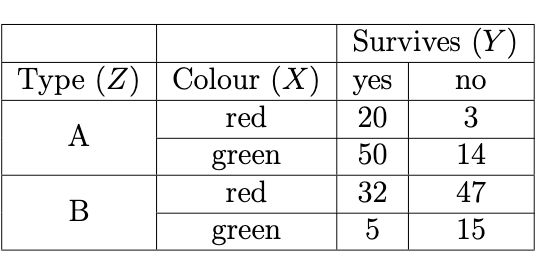
Figure 11.4: Contingency table of the data presented in Q3-6.

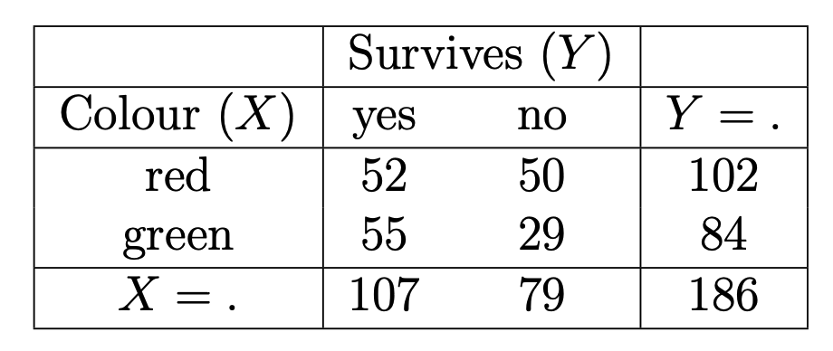
Figure 11.5: Marginal (over Z) XY contingency table.

Calculate an estimate of, along with a \(90\%\) confidence interval for, the marginal odds ratio of Colour and Survives.

Answer: The (local) sample odds ratio (required only when \(i=1, j=1\) in this case) is \[\begin{equation} \hat{r}_{ij} = \frac{n_{i,j,+}n_{i+1,j+1,+}}{n_{i,j+1,+}n_{i+1,j,+}} = \frac{52 \times 29}{50 \times 55} = 0.5484... \end{equation}\]

The corresponding \(90\%\) confidence interval for the log odds ratio is given by: \[\begin{eqnarray} && \log \hat{r}_{ij} \pm z_{1-\alpha/2} \sqrt{\frac{1}{n_{i,j}} + \frac{1}{n_{i+1,j}} + \frac{1}{n_{i,j+1}} + \frac{1}{n_{i+1,j+1}}} \\ & = & \log 0.5484... \pm 1.645 \sqrt{\frac{1}{52} + \frac{1}{55} + \frac{1}{50} + \frac{1}{29}} \\ & = & (-1.0994, -0.1021) \end{eqnarray}\] Therefore, the \(90\%\) confidence interval for the odds ratio is given by: \[\begin{equation} (\exp(-1.0994), \exp(-0.1021)) = (0.3331, 0.9029) \end{equation}\]

What does the estimated odds ratio tell us about the relation between Colour and Survives? Infer whether there is evidence that Colour and Survives are dependent or not.

Answer: The odds ratio suggests a negative association between Colour and Survives, that is, green spacejets typically survive the atmosphere better than red spacejets.

Based on the \(90\%\) confidence interval for the odds ratio, there is evidence to reject the null hypothesis that Colour and Survives are independent at the \(10\%\) level of significance.

Based on the results of Parts (a)-(c), the aliens are convinced that the dataset provides at least some evidence that, regardless of Type, green spacejets have a greater chance of surviving the intense atmospheric pressure than red spacejets. Perform reasonable analyses to:

illustrate to the aliens why they have jumped to the wrong conclusion, and
discuss alternative inferences.

Supposing this was an excerpt from an exam question (as it may have been in the past), credit would be awarded for the clarity of your answer.

Answer:

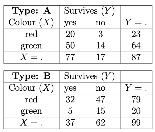
Figure 11.6: Conditional (given Z) XY contingency tables.

Conditional \(XY\)- contingency tables are presented in Figure 11.6, with corresponding conditional sample odds ratios given as follows: \[\begin{equation} \hat{r}_{ij}^{(A)} = \frac{20 \times 14}{50 \times 3} = 1.86... \end{equation}\] \[\begin{equation} \hat{r}_{ij}^{(B)} = \frac{32 \times 15}{47 \times 5} = 2.04... \end{equation}\]

from which we can see that, conditional on Type, there is evidence of a positive association between Colour and Survives, i.e. red Type A spacejets typically survive the atmosphere better than green Type A spacejets, and red Type B spacejets typically survive the atmosphere better than green Type B spacejets.

The alien’s incorrect conclusion arose as a result of marginalising over the confounding factor Type, because this dataset exhibits a phenomenon known as Simpson’s paradox. Simpson’s paradox refers to the case that marginal (over a particular factor) associations are in the opposite direction to every single one of the conditional associations (for each level of the same factor).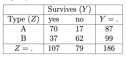

Figure 11.7: Marginal (over X) YZ contingency table.

The marginal \(YZ\) contingency table is presented in Figure 11.7, from which we see that \[\begin{equation} \hat{r}_{jk} = \frac{70 \times 62}{37 \times 17} = 6.90... \end{equation}\] providing evidence of a strong association between Type and Survives, i.e., Type A spacejets have a higher chance of surviving the atmosphere than Type B spacejets.

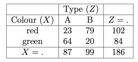
Figure 11.8: Marginal (over Y) XZ contingency table.

Looking at the Marginal \(XZ\) contingency table, presented in Figure 11.8, we see that the marginal sample odds ratio is \[\begin{equation} \hat{r}_{ik} = \frac{23 \times 20}{64 \times 79} = 0.0909... \end{equation}\] suggesting a strong negative association. That is, in this sample, there was a much larger proportion of green Type A spacejets than green Type B spacejets. As a result, when marginalising over Type, green spacejets appeared to have a better survival rate because a bigger proportion of them were Type A.

Q3-7 The Aliens in Durham

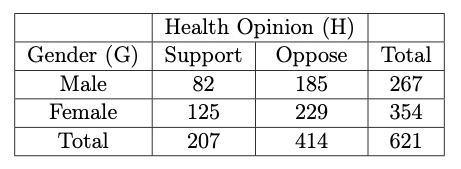
Suppose a horde of 216 aliens (beings from a far-off planet) arrive in Durham and are surveyed about the suitability of building structures were they to make Durham their home (they need to report back to the rest of their species). Suppose the rest of their kind is interested in knowing whether the opinion about suitability is associated with alien height (short, average-height, tall) and alien type (A,B). They therefore cross-classify these variables in the contingency table presented in Figure 10.5.

Calculate an estimate of, along with a \(95\%\) confidence interval for, the marginal odds ratio of Suitability and Type.

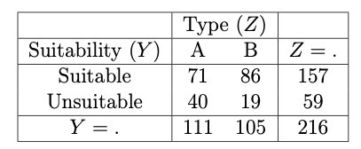
Answer: The Marginal \(YZ\) contingency table (with totals) is presented in Figure 11.9.

Figure 11.9: Marginal (over X) YZ contingency table.

The (local) sample odds ratio (required only when \(j=1, k=1\) in this case) is \[\begin{equation} \hat{r}_{jk} = \frac{n_{+,j,k}n_{+,j+1,k+1}}{n_{+,j+1,k}n_{+,j,k+1}} = \frac{71 \times 19}{40 \times 86} = 0.3922... \end{equation}\] which suggests a negative association between Suitability and Type, that is, Type B aliens typically find Durham more suitable than Type A aliens.

The corresponding \(95\%\) confidence interval for the log odds ratio is given by: \[\begin{eqnarray*} && \log \hat{r}_{jk} \pm z_{1-\alpha/2} \sqrt{\frac{1}{n_{j,k}} + \frac{1}{n_{j+1,k}} + \frac{1}{n_{j,k+1}} + \frac{1}{n_{j+1,k+1}}} \\ & = & \log 0.3922... \pm 1.96 \sqrt{\frac{1}{71} + \frac{1}{40} + \frac{1}{86} + \frac{1}{19}} \\ & = & (-1.566, -0.306) \end{eqnarray*}\] Therefore, the \(95\%\) confidence interval for the odds ratio is given by: \[\begin{equation} (\exp(-1.566), \exp(-0.306)) = (0.209, 0.736) \end{equation}\]

Calculate a minimal set of marginal (over Type) global odds ratios between Height and Suitability, along with a reasonable \(95\%\) confidence interval for each. What assumption about variable Height is being made in order to do this? Interpret and explain the results in terms of associations between Height and Suitability.

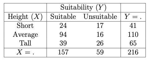
Answer: The Marginal \(XY\) contingency table (with totals) is presented in Figure 11.10.

Figure 11.10: Marginal (over Z) XY contingency table.

The formula for the global odds ratios are typically defined relative to cell \((i,j)\) as \[\begin{equation} r_{ij}^G = \frac{\bigl (\sum_{m \leq i} \sum_{l \leq j} \pi_{ml} \bigr) \bigl (\sum_{m > i} \sum_{l > j} \pi_{ml} \bigr)}{\bigl (\sum_{m \leq i} \sum_{l > j} \pi_{ml} \bigr) \bigl (\sum_{m > i} \sum_{l \leq j} \pi_{ml} \bigr)} \qquad i = 1,...,I-1 \quad j = 1,...,J-1 \end{equation}\] where it is implicitly assumed that any variables with more than two categories (i.e. \(I>2\) or \(J>2\)) are being treated as ordinal.

The sample global odds ratios corresponding to cells \((1,1)\) and \((2,1)\) are therefore given by \[\begin{equation} \hat{r}_{11}^G = \frac{24 \times (16+26)}{(94+39) \times 17} = 0.4458... \qquad \textrm{and} \qquad \hat{r}_{21}^G = \frac{(24 + 94) \times 26}{39 \times (17+16)} = 2.3838... \end{equation}\] respectively, where we are making the assumption that the variable Height can be treated as ordinal.

Each of these odds ratios corresponds to treating Height as a variable with two categories; either resulting from Average being grouped together with Tall (split at \((1,1)\)) or Short (split at \((2,1)\)). Therefore, following from our knowledge of confidence intervals for local odds ratios, the \(95\%\) confidence interval for the global odds ratios corresponding to cells \((1,1)\) and \((2,1)\) are given by \[\begin{equation} \log(0.4458) \pm 1.96 \sqrt{\frac{1}{24} + \frac{1}{16+26} + \frac{1}{94+39} + \frac{1}{17}} = (-1.519, -0.096) \end{equation}\] and \[\begin{equation} \log(2.3838) \pm 1.96 \sqrt{\frac{1}{24+94} + \frac{1}{26} + \frac{1}{39} + \frac{1}{17+16}} = (0.2400, 1.4974) \end{equation}\] respectively.

The fact that \(\hat{r}_{11}^G\) is less than 1 suggests a negative association, that is, group Short is less likely than group Average/Tall to be satisfied with Durham.
The fact that \(\hat{r}_{21}^G\) is greater than 1 suggests a positive association, that is, group Short/Average is more likely than group Tall to be satisfied with Durham.
It might be reasonable to treat Height as ordinal, but the association between Height and Suitability is not linear.
This can be verified by noticing that a greater proportion of the Average height aliens find Durham suitable relative to either Short or Tall aliens.

Chapter 4

Q4-1 Equations from the Notes

By rearranging Equation (4.3), show that Equations (4.6) - (4.9) hold for the 2-way saturated LLM using zero-sum constraints.

Answer:

\[\begin{eqnarray} \log E_{ij} & = & \lambda + \lambda_i^X + \lambda_j^Y + \lambda_{ij}^{XY} \nonumber \\ \implies \sum_{i,j} \log E_{ij} & = & \sum_{i,j} ( \lambda + \lambda_i^X + \lambda_j^Y + \lambda_{ij}^{XY} ) \nonumber \\ & = & IJ \lambda + J \sum_i \lambda_i^{X} + I \sum_j \lambda_j^{Y} + \sum_{i,j} \lambda_{ij}^{XY} \nonumber \\ & = & IJ \lambda \nonumber \\ \implies \lambda = \frac{1}{IJ} \sum_{i,j} \log E_{ij} \end{eqnarray}\] with the final line holding by the zero-sum constraints.

We then have that \[\begin{eqnarray} \sum_{i} \log E_{ij} & = & \sum_{i} ( \lambda + \lambda_i^X + \lambda_j^Y + \lambda_{ij}^{XY} ) \nonumber \\ & = & I \lambda + \sum_i \lambda_i^{X} + I \lambda_j^Y + \sum_i \lambda_{ij}^{XY} \nonumber \\ \implies \lambda_j^Y & = & \frac{1}{I} \sum_{i} \log E_{ij} - \lambda \end{eqnarray}\] and by symmetry also that \[\begin{equation} \lambda_i^X = \frac{1}{J} \sum_{j} \log E_{ij} - \lambda \end{equation}\]

The final equation is shown by a trivial rearrangement: \[\begin{equation} \lambda_{ij}^{XY} = \log E_{ij} - \lambda - \lambda_i^X - \lambda_j^Y \end{equation}\]

Assuming Equation (4.12) holds, for the 2-way independence LLM, show that the ML estimates for the \(\lambda\) parameters are as given by Equations (4.13) - (4.15).

Answer: For the independence model, we have that \[\begin{equation} \hat{E}_{ij} = \frac{\hat{E}_{i+}\hat{E}_{+j}}{n_{++}} = \frac{n_{i+}n_{+j}}{n_{++}} \end{equation}\] following Section 2.4.3.2.

Then, we can substitute these estimates into Equations (4.6) - (4.9) to obtain MLEs for the \(\lambda\) parameters. \[\begin{eqnarray} \hat{\lambda} & = & \frac{1}{IJ} \sum_{s,t} \log \hat{E}_{st} \nonumber \\ & = & \frac{1}{IJ} \sum_{s,t} \log \frac{n_{s+}n_{+t}}{n_{++}} \nonumber \\ & = & \frac{1}{I} \sum_s \log n_{s+} + \frac{1}{J} \sum_t \log n_{+t} - \log n_{++} \nonumber \\ \hat{\lambda}_{i+} & = & \frac{1}{J} \sum_t \log \hat{E}_{st} - \hat{\lambda} \nonumber \\ & = & \frac{1}{J} \sum_t \log \frac{n_{s+}n_{+t}}{n_{++}} - \hat{\lambda} \nonumber \\ & = & \frac{1}{J} (J \log n_{s+} + \sum_t \log n_{+t} - \log n_{++}) - \hat{\lambda} \nonumber \\ & = & \log n_{s+} + \frac{1}{J} \sum_t \log n_{+t} - \frac{1}{J} \log n_{++} - \bigl( \frac{1}{I} \sum_s \log n_{s+} + \frac{1}{J} \sum_t \log n_{+t} - \log n_{++} \bigr) \nonumber \\ & = & \log n_{s+} - \frac{1}{I} \sum_s \log n_{s+} \qquad i = 1,...,I \end{eqnarray}\] and by symmetry: \[\begin{equation} \hat{\lambda}_{+j} = \log n_{+t} - \frac{1}{J} \sum_s \log n_{+t} \qquad j = 1,...,J \end{equation}\]

Q4-2: Two-way Mutual Independence Model

Assume a LLM with dependency structure \([X,Y]\) under a Poisson sampling scheme with corner point constraints.

Write down the appropriate LLM expression corresponding to dependency structure \([X,Y]\).

Answer: We have that \[\begin{equation} \log(E_{ij}) = \lambda + \lambda^X_i + \lambda^Y_j \end{equation}\]

Rearrange the appropriate LLM expression for the corresponding \(\lambda\) parameters⁸⁴.

Answer: In this question we assume corner point constraints with reference categories \(I\) and \(J\), so that \[\begin{equation} \lambda^X_I = \lambda^Y_J = 0 \end{equation}\]

We therefore have that \[\begin{eqnarray} \log(E_{IJ}) & = & \lambda + \lambda^X_I + \lambda^Y_J = \lambda \nonumber \\ \log(E_{Ij}) & = & \lambda + \lambda^X_I + \lambda^Y_j = \lambda + \lambda^Y_j \nonumber \\ \log(E_{iJ}) & = & \lambda + \lambda^X_i + \lambda^Y_J = \lambda + \lambda^X_i \nonumber \end{eqnarray}\] so that \[\begin{eqnarray} \lambda & = & \log(E_{IJ}) \nonumber \\ \lambda^X_i & = & \log(E_{iJ}) - \lambda = \log(\frac{E_{iJ}}{E_{IJ}}) \nonumber \\ \lambda^Y_j & = & \log(E_{Ij}) - \lambda = \log(\frac{E_{Ij}}{E_{IJ}}) \nonumber \end{eqnarray}\]

Write down the log-likelihood equations, and hence use the method of Lagrange multipliers to show that \[\begin{eqnarray} \hat{E}_{++} = E_{++}(\hat{\boldsymbol{\lambda}}) & = & n_{++} \nonumber \\ \hat{E}_{i+} = E_{i+}(\hat{\boldsymbol{\lambda}}) & = & n_{i+} \qquad i = 1,...,I \nonumber \\ \hat{E}_{+j} = E_{+j}(\hat{\boldsymbol{\lambda}}) & = & n_{+j} \qquad j = 1,...,J \nonumber \end{eqnarray}\]

Answer:

The log-likelihood expression is given by⁸⁵ \[\begin{eqnarray} l(\boldsymbol{\lambda}) & \propto & \sum_{i,j} (n_{ij} \log E_{ij} - E_{ij}) \nonumber \\ & = & \sum_{i,j} (n_{ij} (\lambda + \lambda_i^X + \lambda_j^Y) - E_{ij}(\lambda)) \nonumber \\ & = & n_{++} \lambda + \sum_{i} n_{i+} \lambda_i^X + \sum_{j} n_{+j} \lambda_j^Y - \sum_{i,j} E_{ij}(\lambda) \nonumber \end{eqnarray}\] where I define \[\begin{equation} E_{ij}(\lambda) = \exp(\lambda + \lambda_i^X + \lambda_j^Y) \nonumber \end{equation}\]

The Lagrange function is then \[\begin{equation} \mathcal{L}(\boldsymbol{\lambda}, \boldsymbol{\theta}) = n_{++} \lambda + \sum_i n_{i+} \lambda_i^X + \sum_{j} n_{+j} \lambda_j^Y - \sum_{i,j} E_{ij}(\lambda) - \theta^X \lambda_I^X - \theta^Y \lambda_J^Y \end{equation}\]

We now need to calculate the derivative of \(\mathcal{L}(\boldsymbol{\lambda}, \boldsymbol{\theta})\) with respect to each parameter and set equal to \(0\). We have \[\begin{eqnarray} \frac{\partial \mathcal{L}(\hat{\boldsymbol{\lambda}}, \hat{\boldsymbol{\theta}})}{\partial \lambda} & = & n_{++} - \sum_{i,j} E_{ij}(\hat{\lambda}) = 0 \nonumber \\ \implies E_{++}(\hat{\boldsymbol{\lambda}}) & = & n_{++} \nonumber \\ \frac{\partial \mathcal{L}(\hat{\boldsymbol{\lambda}}, \hat{\boldsymbol{\theta}})}{\partial \lambda_i^X} & = & n_{i+} - \sum_{j} E_{ij}(\hat{\lambda}) = 0 \qquad i = 1,...,I-1 \nonumber \\ \implies E_{i+}(\hat{\boldsymbol{\lambda}}) & = & n_{i+} \qquad i = 1,...,I-1 \nonumber \\ \frac{\partial \mathcal{L}(\hat{\boldsymbol{\lambda}}, \hat{\boldsymbol{\theta}})}{\partial \lambda_I^X} & = & n_{I+} - \sum_{j} E_{Ij}(\hat{\lambda}) - \hat{\theta}^X = 0 \nonumber \\ \implies n_{I+} & = & E_{I+}(\hat{\boldsymbol{\lambda}}) + \hat{\theta}^X \nonumber \\ \frac{\partial \mathcal{L}(\hat{\boldsymbol{\lambda}}, \hat{\boldsymbol{\theta}})}{\partial \lambda_j^Y} & = & n_{+j} - \sum_{i} E_{ij}(\hat{\lambda}) = 0 \qquad j = 1,...,J-1 \nonumber \\ \implies E_{+j}(\hat{\boldsymbol{\lambda}}) & = & n_{+j} \qquad j = 1,...,J-1 \nonumber \\ \frac{\partial \mathcal{L}(\hat{\boldsymbol{\lambda}}, \hat{\boldsymbol{\theta}})}{\partial \lambda_J^Y} & = & n_{+J} - \sum_{i} E_{iJ}(\hat{\lambda}) - \hat{\theta}^Y = 0 \nonumber \\ \implies n_{+J} & = & E_{+J}(\hat{\boldsymbol{\lambda}}) + \hat{\theta}^Y \nonumber \\ \frac{\partial \mathcal{L}(\hat{\boldsymbol{\lambda}}, \hat{\boldsymbol{\theta}})}{\partial \theta^X} & = & - \lambda_I^X = 0 \nonumber \\ \frac{\partial \mathcal{L}(\hat{\boldsymbol{\lambda}}, \hat{\boldsymbol{\theta}})}{\partial \theta^Y} & = & - \lambda_J^Y = 0 \nonumber \end{eqnarray}\] From the above equations, we have that \[\begin{eqnarray} \sum_{i=1}^I E_{i+}(\hat{\boldsymbol{\lambda}}) + \hat{\theta}^X & = & \sum_{i=1}^I n_{i+} \nonumber \\ n_{++} & = & E_{++}(\hat{\boldsymbol{\lambda}}) + \hat{\theta}^X \nonumber \\ \implies \hat{\theta}^X & = & 0 \nonumber \\ \sum_{j=1}^J E_{+j}(\hat{\boldsymbol{\lambda}}) + \hat{\theta}^Y & = & \sum_{j=1}^J n_{+j} \nonumber \\ n_{++} & = & E_{++}(\hat{\boldsymbol{\lambda}}) + \hat{\theta}^Y \nonumber \\ \implies \hat{\theta}^Y & = & 0 \end{eqnarray}\] so that \[\begin{eqnarray} n_{I+} & = & E_{I+}(\hat{\boldsymbol{\lambda}}) \nonumber \\ n_{+J} & = & E_{I+}(\hat{\boldsymbol{\lambda}}) \end{eqnarray}\] as required.⁸⁶

Using the results of parts (b) and (c), or otherwise, find the MLEs of the LLM \(\lambda\) coefficients.

Answer: The numbering of steps below correspond to the outline algorithm of Section 4.4.

Step 1: Answer to part (b).

Step 2: Model \([X,Y]\) is defined by \[\begin{equation} \pi_{ij} = \pi_{i+} \pi_{+j} \implies E_{ij} = \frac{E_{i+}E_{+j}}{n_{++}} \end{equation}\]

Step 3: Answer to part (c).

Step 4: The MLEs are therefore \[\begin{equation} \hat{E}_{ij} = \frac{\hat{E}_{i+}\hat{E}_{+j}}{n_{++}} = \frac{n_{i+}n_{+j}}{n_{++}} \end{equation}\] by the results of parts (c).

Step 5: Finally, we can substitute these MLEs in to the expressions for \(\boldsymbol{\lambda}\) obtained in part (b), to obtain: \[\begin{eqnarray} \hat{\lambda} & = & \log(\hat{E}_{IJ}) = \log(\frac{n_{I+}n_{+J}}{n_{++}}) \nonumber \\ \hat{\lambda}_i^X & = & \log(\frac{\hat{E}_{iJ}}{\hat{E}_{IJ}}) = \log(\frac{n_{i+}}{n_{I+}}) \nonumber \\ \hat{\lambda}_j^Y & = & \log(\frac{\hat{E}_{Ij}}{\hat{E}_{IJ}}) = \log(\frac{n_{+j}}{n_{+J}}) \nonumber \end{eqnarray}\]

Q4-3: Hierarchical Log Linear Models

Identify if the following models are hierarchical, and for the ones that are, use the square bracket \([]\) notation (e.g. \([X,Y]\) for the two-way independence model) presented throughout Sections 3 and 4 to represent them, and discuss what assumptions about the associations between the variables they convey:

\[\begin{eqnarray} \textrm{i. } \log E_{ijk} & = & \lambda + \lambda_i^X + \lambda_j^Y + \lambda_k^Z + \lambda_{jk}^{YZ} \qquad \forall i,j,k \nonumber \\ \textrm{ii. } \log E_{ijkl} & = & \lambda + \lambda_i^X + \lambda_j^Y + \lambda_k^Z + \lambda_l^W + \lambda_{ij}^{XY} + \lambda_{il}^{XW} + \lambda_{kl}^{ZW} + \lambda_{ikl}^{XZW} \qquad \forall i,j,k,l \nonumber \\ \textrm{iii. }\log E_{ijkl} & = & \lambda + \lambda_i^X + \lambda_j^Y + \lambda_k^Z + \lambda_l^W + \lambda_{ik}^{XZ} + \lambda_{il}^{XW} + \lambda_{kl}^{ZW} + \lambda_{ikl}^{XZW} \qquad \forall i,j,k,l \nonumber \end{eqnarray}\]

Answer:

\([X, YZ]\) - \(X\) is jointly independent with both \(Y\) and \(Z\) (but \(Y\) and \(Z\) (could⁸⁷) interact with each other).
This is not a hierarchical log-linear model due to the presence of a \(\lambda_{ikl}^{XZW}\) term but the absence of a \(\lambda_{ik}^{XZ}\) term.
\([Z, XYW]\) - \(Z\) is jointly independent with \(X\), \(Y\) and \(W\), but these three variables (could) exhibit full (three-way) interaction with each other.

Write down the hierarchical log-linear models corresponding to

\([XY, XZ]\)
\([XY, XZ, XW]\)
\([X_1X_3, X_2X_3X_4, X_4X_5, X_5X_6]\)

and discuss what assumptions about the associations between the variables they convey.

Answer:

\[\begin{equation} \textrm{i. } \log E_{ijk} = \lambda + \lambda_i^X + \lambda_j^Y + \lambda_k^Z + \lambda_{ij}^{XY} + \lambda_{ik}^{XZ} \qquad \forall i,j,k \end{equation}\] which models \(Y\) and \(Z\) as being conditionally independent given \(X\).

\[\begin{equation} \textrm{ii. } \log E_{ijk} = \lambda + \lambda_i^X + \lambda_j^Y + \lambda_k^Z + \lambda_l^{W} + \lambda_{ij}^{XY} + \lambda_{ik}^{XZ} + \lambda_{il}^{XW} \qquad \forall i,j,k \end{equation}\] which models \(Y, Z\) and \(W\) as being conditionally (given \(X\)) mutually independent. Note that \(Y, Z\) and \(W\) may not be marginally mutually independent given \(X\).

\[\begin{eqnarray} \textrm{iii. } \log E_{i_1...i_6} & = & \lambda + \lambda_{i_1}^{X_1} + \lambda_{i_2}^{X_2} + \lambda_{i_3}^{X_3} + \lambda_{i_4}^{X_4} + \lambda_{i_5}^{X_5} + \lambda_{i_6}^{X_6} \nonumber \\ && + \lambda_{i_1i_3}^{X_1X_3} + \lambda_{i_2i_3}^{X_2X_3} + \lambda_{i_2i_4}^{X_2X_4} + \lambda_{i_3i_4}^{X_3X_4} + \lambda_{i_4i_5}^{X_4X_5} + \lambda_{i_5i_6}^{X_5X_6} \nonumber \\ && + \lambda_{i_2i_3i_4}^{X_2X_3X_4} \qquad \forall i_1,i_2,i_3,i_4,i_5,i_6,i_7 \tag{11.8} \end{eqnarray}\] which models a three-way interaction between variables \(X_2, X_3\) and \(X_4\), with additional two-way interactions between \(X_1\) and \(X_3\), \(X_4\) and \(X_5\), and \(X_5\) and \(X_6\).

For the model discussed in part b-iii above, are variables \(X_1\) and \(X_6\) necessarily independent? Explain your answer.

Answer: \(X_1\) and \(X_6\) are not in general (i.e. marginally over \(X_5\)) independent. \(X_1\) and \(X_6\) are conditionally independent given \(X_5\). In other words, \(X_1\) and \(X_6\) (may) interact with each other, but this interaction can be captured and explained through the value of \(X_5\).

Q4-4: 1988 General Social Survey

The 1988 General Social Survey compiled by the National Opinion Research Center asked:

“Do you support or oppose the following measures to deal with AIDS? (1) Have the government pay all of the health care costs of AIDS patients; (2) Develop a government information program to promote safe sex practices, such as the use of condoms.”

The table in Figure 10.3 summarizes opinions about health care costs (H) and the information program (I), classified also by the respondent’s gender (G).

Regarding the questions below, any inference based on hypothesis tests should be performed at the \(5\%\) level of significance.

By using appropriate statistical tools, compare the following associations of the classification variables.

mutual independence of \(X, Y\) and \(Z\), against
conditional independence of \(X\) and \(Y\) on \(Z\).

Justify the way you address the problem.

Answer: This is a comparison between nested models, so I’ll perform a LRT of the following hypotheses: \[\begin{align} \mathcal{H}_0: & \, \mathcal{M}_0: [X,Y,Z] \\ \mathcal{H}_1: & \, \mathcal{M}_1: [XZ, YZ] \end{align}\]

The likelihood ratio test statistic is \[\begin{equation} G^2(\mathcal{M}_0, \mathcal{M}_1) = 2 \sum_{i,j,k} n_{ijk} \log \bigl( \frac{\hat{E}^{(1)}_{ijk}}{\hat{E}^{(0)}_{ijk}} \bigr) \sim \chi^2_{df} \end{equation}\] where \[\begin{eqnarray} \hat{E}^{(0)}_{ijk} & = & \frac{n_{i++}n_{+j+}n_{++k}}{n_{+++}^2} \\ \hat{E}^{(1)}_{ijk} & = & \frac{n_{i+k}n_{+jk}}{n_{++k}} \\ df & = & (I-1)(K-1) + (I-1)(J-1) = 2 \end{eqnarray}\] since the two models differ only in terms of the parameters \(\lambda_{ik}^{XZ}\) and \(\lambda_{ij}^{XY}\).

Let \[\begin{equation} G_{ijk} = 2 n_{ijk} \log \bigl( \frac{\hat{E}^{(1)}_{ijk}}{\hat{E}^{(0)}_{ijk}} \bigr) \end{equation}\]

In order to calculate the \(G_{ijk}\), I calculate the quantities in the table given in Figure 11.11.

Figure 11.11: Quantities required for Question 4-3a.

Therefore \(G^2_{obs} = \sum_{i,j,k} G_{ijk} = 4.652218\).

The critical value is \(\chi_{2,0.95}^2 = 5.991\), therefore the test does not reject the null hypothesis model of mutual independence in favour of model \(\mathcal{M}_1\) at the \(5\%\) level of significance.

By using appropriate statistical tools, compare the following associations of the classification variables

joint independence of \(X\) and \(Z\) on \(Y\), against
joint independence of \(X\) and \(Y\) on \(Z\).

Justify the way you address the problem.

Answer: This is a comparison between non-nested models, so I will use information criteria for comparison purposes. For the purposes of this question, let’s compare using both AIC and BIC.

\[\begin{eqnarray} \textrm{AIC}(\mathcal{M}) & = & -2 l_{\mathcal{M}}(\hat{\lambda}) + 2 d_{\mathcal{M}} \\ \textrm{BIC}(\mathcal{M}) & = & - 2 l_{\mathcal{M}}(\hat{\lambda}) + \log(n_{+++}) d_{\mathcal{M}} \end{eqnarray}\]

Joint independence of \(X\) and \(Z\) on \(Y\) is given by model \(\mathcal{M}_A: [XZ, Y]\). Assuming Poisson sampling, we have that \[\begin{equation} l_{\mathcal{M}_A}(\hat{\lambda}) = \sum_{ijk} ( -\hat{E}^A_{ijk} + n_{ijk} \log \hat{E}^A_{ijk} - \log n_{ijk}! ) \propto - n_{+++} + \sum_{ijk} n_{ijk} \log \hat{E}^A_{ijk} \end{equation}\] where \[\begin{equation} \hat{E}^A_{ijk} = \frac{n_{i+k}n_{+j+}}{n_{+++}} \end{equation}\] and \(d_{\mathcal{M_A}} = 1 + (I-1) + (J-1) + (K-1) + (I-1)(K-1) = 5\).

Joint independence of \(X\) and \(Y\) on \(Z\) is given by model \(\mathcal{M}_B: [XY, Z]\). Assuming Poisson sampling, we have that \[\begin{equation} l_{\mathcal{M}_B}(\hat{\lambda}) = \sum_{ijk} ( -\hat{E}^B_{ijk} + n_{ijk} \log \hat{E}^B_{ijk} - \log n_{ijk}! ) \propto - n_{+++} + \sum_{ijk} n_{ijk} \log \hat{E}^B_{ijk} \end{equation}\] where \[\begin{equation} \hat{E}^B_{ijk} = \frac{n_{ij+}n_{++k}}{n_{+++}} \end{equation}\] and \(d_{\mathcal{M_B}} = 1 + (I-1) + (J-1) + (K-1) + (I-1)(J-1) = 5\).

Figure 11.12: Quantities required for Question 4-3b.

Figure 11.13: Quantities required for Question 4-3b.

Using the quantities calculated in the tables presented in Figures 11.12 and 11.13, we have that \[\begin{eqnarray} AIC(\mathcal{M}_A) & \propto & -4584.997 \\ AIC(\mathcal{M}_B) & \propto & -4592.519 \\ BIC(\mathcal{M}_A) & \propto & -4562.844 \\ BIC(\mathcal{M}_B) & \propto & -4570.365 \end{eqnarray}\]

Both AIC and BIC indicate that model \(\mathcal{M}_B:[XY,Z]\) is preferable.

Q4-5: \(2 \times 2 \times 2\) Contingency Table

Consider a \(2 \times 2 \times 2\) Contingency Table with classification variables \(X\), \(Y\) and \(Z\).

State the equation of the Log-linear model describing the dependency type \([XY,XZ]\).

Answer: This model describes the dependency type \(Z\) and \(Y\) being conditionally independent on \(X\). It is given by the following LLM: \[\begin{equation} \log E_{ijk} = \lambda + \lambda_i^X + \lambda_j^Y + \lambda_k^Z + \lambda_{ij}^{XY} + \lambda_{ik}^{XZ} \qquad \forall (i,j,k) \in \{1,2\} \end{equation}\]

Apply the two types of the non-identifiability constraints (corner points and sum-to-zero).

Answer: The corner point constraints, with reference levels \(i=2, j=2, k=2\), are \[\begin{eqnarray} \lambda_2^X = \lambda_2^Y = \lambda_2^Z & = & 0 \\ \lambda_{2j}^{XY} = \lambda_{i2}^{XY} & = & 0 \quad \forall i,j \\ \lambda_{2k}^{XZ} = \lambda_{i2}^{XZ} & = & 0 \quad \forall i,k \end{eqnarray}\]

The sum-to-zero constraints are given by \[\begin{eqnarray} \lambda_1^X & = & - \lambda_2^X \\ \lambda_1^Y & = & - \lambda_2^Y \\ \lambda_1^Z & = & - \lambda_2^Z \\ \lambda_{i1}^{XY} & = & - \lambda_{i2}^{XY} \quad \forall i \\ \lambda_{1j}^{XY} & = & - \lambda_{2j}^{XY} \quad \forall j \\ \lambda_{i1}^{XZ} & = & - \lambda_{i2}^{XZ} \quad \forall i \\ \lambda_{1k}^{XZ} & = & - \lambda_{2k}^{XZ} \quad \forall k \\ \end{eqnarray}\]

Write down the number of free parameters, and explain how you calculated them.

Answer: The number of free parameters is given by \[\begin{eqnarray} d & = & 1 + (I-1) + (J-1) + (K-1) + (I-1)(J-1) + (I-1)(K-1) \\ & = & 1 + (2-1) + (2-1) + (2-1) + (2-1)(2-1) + (2-1)(2-1) = 6 \end{eqnarray}\]

because

from \(\lambda\) I have 1 free parameters
from \(\lambda_i^X\) I have \(I=2\) parameters, but because of the constraints one of them is set to zero or can be specified from the others. Same goes for \(\lambda_j^Y\) and \(\lambda_k^Z\).
from \(\lambda_{ik}^{XZ}\) I have \(I \times K = 2 \times 2 = 4\) parameters, but because of the constraints \(I + K - 1 = 3\) of them are set to zero or can be specified from the others. Same goes for \(\lambda_{ij}^{XY}\).

For parts (d) and (e), consider the corner point constraints only.

Express \(\log(\pi_{1|jk} / \pi_{2|jk})\) as a function of the linear model \(\lambda\) coefficients.

Answer: We have that \[\begin{equation} \log(\pi_{1|jk} / \pi_{2|jk}) = \log(E_{1jk} / E_{2jk}) = \log(E_{1jk}) - \log(E_{2jk}) = \begin{cases} \lambda_1^X + \lambda_{11}^{XY} + \lambda_{11}^{XZ}, & j = 1, k = 1 \\ \lambda_1^X + \lambda_{11}^{XY}, & j = 1, k = 2 \\ \lambda_1^X + \lambda_{11}^{XZ} , & j = 2, k = 1 \\ \lambda_1^X , & j = 2, k = 2 \end{cases} \end{equation}\]

Express \(\log(r^{XY}_{ij(k)})\), that is, the log conditional (on \(Z\)) odds ratio, as a function of the linear model \(\lambda\) coefficients. Give a short interpretation of \(\lambda_{11}^{XY}\) based on this.

Answer: We have that \[\begin{equation} \log(r^{XY}_{ij(k)}) = \log(\frac{E_{11k}/E_{21k}}{E_{12k}/E_{22k}}) = \lambda_{11}^{XY} \quad \forall k \end{equation}\] hence \(\lambda_{11}^{XY}\) is equal to the log conditional (on \(Z\)) odds ratio of \(X\) to \(Y\), for any level of \(Z\).

Q4-6: Exam-Style Question

All possible hierarchical log-linear models were fitted to a contingency table, based on a sample of 312 individuals, for three factors: X (2 levels), Y (3 levels) and Z (5 levels). The sampling scheme that was implemented was the Poisson sampling scheme. The results are shown in the table in Figure 10.6.

Calculate the number of free parameters resulting after applying corner point non-identifiability constraints for each model in the table.

Answer: The number of the free parameters resulting after applying corner point non- identifiability constraints for each model is in the 3rd column of the table in Figure 11.14. These are for the Poisson sampling scheme.

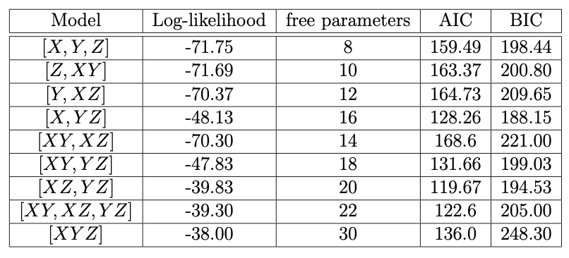
Figure 11.14: Table for Q4-5.

Define the Akaike Information Criterion (AIC) and Bayes Information Criterion (BIC), then compute both AIC and BIC for each model in the table.

For model \(\mathcal{M}\), the Akaike Information Criterion (AIC), is given by \[\begin{equation} AIC(\mathcal{M}) = -2 l_{\mathcal{M}}(\hat{\boldsymbol{\lambda}}) + 2 d_{\mathcal{M}} \end{equation}\] where \(l_{\mathcal{M}}(\hat{\boldsymbol{\lambda}})\) is the value of the log-likelihood function at the MLE for \(\boldsymbol{\lambda}\) for the appropriate set of \(\lambda\) parameters corresponding to model \(\mathcal{M}\), and \(d_{\mathcal{M}}\) is the number of free parameters in model \(\mathcal{M}\). The Bayesian Information Criterion (BIC), is given by \[\begin{equation} BIC(\mathcal{M}) = -2 l_{\mathcal{M}}(\hat{\boldsymbol{\lambda}}) + \log(n_{+...+}) d_{\mathcal{M}} \end{equation}\] where additionally here we define \(n_{+...+}\) to be the total number of observations.

The Akaike Information Criterion (AIC) and Bayes Information Criterion (BIC) are calculated and presented in the 4th and 5th columns respectively of the table in Figure 11.14.

Identify which model is selected by each criterion and give a short explanation of what each criterion is intended to achieve.

Using criterion AIC would lead to selecting model \([XZ,YZ]\), while using criterion BIC would lead to selecting model \([X,YZ]\).

Both AIC and BIC seek to maximise the likelihood subject to a penalty on the complexity of the model in terms of the number of parameters. If \(AIC(\mathcal{M}_1)>AIC(\mathcal{M}_2)\) then model \(\mathcal{M}_2\) is preferable to model \(\mathcal{M}_1\) according to criterion AIC. If \(BIC(\mathcal{M}_1) > BIC(\mathcal{M}_2)\) then model \(\mathcal{M}_2\) is preferable to model \(\mathcal{M}_1\) according to criterion BIC.

Explain precisely what model \([XY,YZ]\) says about the dependence of factor \(Y\) on the other two factors.

Model \([XY, YZ]\) means that \(X\) and \(Z\) are conditionally independent given \(Y\).

Chapter 5

Q5-1: Tokyo Rainfall

We consider rainfall data recorded in Tokyo in the first 11 days of the year 1983, as given by the table in Figure 10.7. For each day, we know whether it rained (\(z_i=1)\) or did not rain (\(z_i=0\)) on that day.

The goal is to find a model which predicts the probability of rain on day \(i+1\) based on the rainfall on day \(i\), which is given by \(z_i\). Therefore, we define the response \(y_i=z_{i+1}\), \(i=1, \ldots, 10\), so that we can write the data in the form given by the table in Figure 10.8

Formulate a logistic regression model for \(\pi(z)\) (consider the elements stated in Section 5.3.2), using the linear predictor \(\eta=\beta_{1}+\beta_{2} z\), that is, take the predictors to be \(x_{1} \equiv 1\) and \(x_{2} = z\).

Answer: The elements of the logistic regression model are as follows:

Linear predictor: \(\eta(z) = \beta_{1} + \beta_{2} z\), for \(z\in\{0, 1\}\).
Response function \(h(\eta) = \frac{\exp(\eta)}{1+\exp(\eta)}\).
Distributional assumption: \(y |\boldsymbol{\beta}, z \sim \text{Bern}(\pi(z))\), where \(\pi(z) = h(\eta(z))\). One could also add that, given \(z_{i}\) (and \(\beta\)), each \(y_{i}\) is independent of the other \(y_{j}\) and \(z_{j}\), \(j\neq i\).

Since \(z\) only takes on two values, \(0\) and \(1\), there are only two values of \(\pi(z)\), which we call \(\pi_{0} = \pi(0)\) and \(\pi_{1} = \pi(1)\).

Formulate the score function \(S(\boldsymbol{\beta})\).

Answer: The general formula for the score function for the logistic model is: \[\begin{equation} S(\boldsymbol{\beta}) = \sum_{i = 1}^{n} (y_{i} - \pi(\boldsymbol{x}_{i})) \boldsymbol{x}_{i} \end{equation}\]

Here, \(\boldsymbol{x}_{i} = (1, z_{i})\), where each of the \(z_{i}\in\{0, 1\}\). So we have \[\begin{align} S(\boldsymbol{\beta}) = \sum_{i:\,z_{i} = 0} (y_{i} - \pi_{0}) \begin{pmatrix} 1 \\ 0 \end{pmatrix} + \sum_{i:\,z_{i} = 1} (y_{i} - \pi_{1}) \begin{pmatrix} 1 \\ 1 \end{pmatrix} \end{align}\]

Solve the estimating equation \(S(\hat{\boldsymbol{\beta}})=0\).

Answer: Setting \(S(\hat{\boldsymbol{\beta}}) = 0\) gives two equations: \[\begin{align} 0 & = \sum_{i:\,z_{i} = 0} (y_{i} - \hat{\pi}_{0}) + \sum_{i:\,z_{i} = 1} (y_{i} - \hat{\pi}_{1}) \\ 0 & = \sum_{i:\,z_{i} = 1} (y_{i} - \hat{\pi}_{1}) \end{align}\]

Let \(n_{b} = \sum_{i:\,z_{i} = b} 1\), and \(\bar{y}_{b} = \tfrac{1}{n_{b}}\sum_{i:\,z_{i} = b} y_{i}\), for \(b\in\{0, 1\}\). Then the above equations give: \[\begin{align} 0 & = n_{0}(\bar{y}_{0} - \hat{\pi}_{0}) + n_{1}(\bar{y}_{1} - \hat{\pi}_{1}) \\ 0 & = n_{1}(\bar{y}_{1} - \hat{\pi}_{1}) \end{align}\]

This gives immediately that \[\begin{equation} \hat{\pi}_{b} = \bar{y}_{b} \end{equation}\] for \(b\in\{0, 1\}\). Note that this is just the proportion of rainy days following a non-rainy (\(b = 0\)) or a rainy (\(b = 1\)) day, as you might expect.

Now we have to solve for \(\hat{\boldsymbol{\beta}}\). We have: \[\begin{align} \hat{\pi}_{0} & = \frac{e^{\hat{\beta}_{1}}}{1 + e^{\hat{\beta}_{1}}} \\ \hat{\pi}_{1} & = \frac{e^{\hat{\beta}_{1} + \hat{\beta}_{2}}}{1 + e^{\hat{\beta}_{1} + \hat{\beta}_{2}}} \end{align}\]

This gives: \[\begin{align} \hat{\beta}_{1} & = \log \frac{\hat{\pi}_{0}}{1 - \hat{\pi}_{0}} \\ \hat{\beta}_{1} + \hat{\beta}_{2} & = \log \frac{\hat{\pi}_{1}}{1 - \hat{\pi}_{1}} \end{align}\] whence it is easy to find \(\hat{\beta}_{2}\).

In this particular case, we have \(\bar{y}_{0} = \tfrac{2}{6} = \tfrac{1}{3}\) and \(\bar{y}_{1} = \tfrac{2}{4} = \tfrac{1}{2}\), which then gives that \[\begin{align} \hat{\beta}_{1} & = -0.6931472 \\ \hat{\beta}_{2} & = 0.6931472 \end{align}\]

An important point must be made here. We can only solve the equations for the \(\hat{\pi}_{b}\) first because there are as many \(\hat{\pi}\) probabilities as there are \(\hat{\beta}\) parameters (two). In a more complex model, there will generally be an infinite set of \(\hat{\pi}_{i}\) (or more generally means \(\hat{\mu}_{i}\)) satisfying the equations \[\begin{equation} \sum_{i} (y_{i} - \hat{\pi}_{i})\boldsymbol{x}_{i} = 0 \end{equation}\] simply because there are \(p\) equations and \(n\) unknowns. However, only one of this infinite set can be written in the form \(h(\hat{\boldsymbol{\beta}}^{T}\boldsymbol{x}_{i})\), for which there are only \(p\) unknowns, corresponding to the \(\hat{\beta}\) parameters.

According to BBC Weather, it didn’t rain in Tokyo on Thursday November 17, 2022. Use your model to predict the rainfall probability in Tokyo on Friday November 18, 2022.

Answer: On 17/11/2022, we observed the covariate value \(z = 0\). Hence the predicted probability of rain on 18/11/2022 is \[\begin{equation} \hat{\pi}_{0} = \bar{y}_{0} = \frac{e^{\hat{\beta}_{1}}}{1 + e^{\hat{\beta}_{1}}} = \frac{1}{3} \end{equation}\]

Chapter 6

Q6-1: Properties of the Exponential Dispersion Family

Let the distribution for \(Y\) be an exponential dispersion family: \[\begin{equation} P_{}\left(y |\theta(\mu), \phi\right) = \exp \bigl[ \frac{y\theta(\mu) - b(\theta(\mu))}{ \phi} + c(y, \phi) \bigr] \end{equation}\]

where \(\mu(\theta) = {\mathrm E}[Y |\theta, \phi]\).

Use the fact that \(\mu(\theta)\) and \(\theta(\mu)\) are inverses to show that \(\theta'(\mu) = 1/\mathcal{V}(\mu)\), where \(\mathcal{V}(\mu)\) is the variance function.

Answer: The fact that \(\mu\) and \(\theta\) are inverses means that \[\begin{equation} \mu = \mu(\theta(\mu)) \end{equation}\]

Differentiating both sides with respect to \(\mu\) gives \[\begin{equation} 1 = \mu'(\theta(\mu)) \;\theta'(\mu) \end{equation}\] and hence that \[\begin{equation} \theta'(\mu) = \frac{1}{\mu'(\theta(\mu))} \end{equation}\]

Since \(\mu(\theta) = b'(\theta)\), this gives that \[\begin{equation} \theta'(\mu) = \frac{1}{b''((b')^{-1})(\mu)} = \frac{1}{\mathcal{V}(\mu)} \end{equation}\]

Show that with one data point \((\boldsymbol{x}, y)\), the maximum likelihood estimator for \(\mu\) is \(y\).

Answer: The log likelihood is \[\begin{equation} \ell(y |\mu) = \frac{1}{\phi} (y\;\theta(\mu) - b(\theta(\mu))) + c(y, \phi) \end{equation}\]

Differentiating with respect to \(\mu\), setting the result equal to zero, and multiplying by \(\phi\), then gives \[\begin{equation} y\;\theta'(\hat{\mu}) - b'(\theta(\hat{\mu}))\;\theta'(\hat{\mu}) = 0 \end{equation}\] and hence, if \(\theta'(\hat{\mu})\neq 0\), that \[\begin{equation} y = b'(\theta(\hat{\mu})) = \hat{\mu} \end{equation}\]

Chapter 7

Q7-1: The Gamma Distribution

We consider the exponential dispersion family (EDF)

\[\begin{equation} P(y | \theta, \phi) = \exp\{\frac{y \theta- b(\theta)}{\phi} + c(y, \phi) \} \qquad y>0 \end{equation}\]

Show that the expectation of a distribution belonging to a EDF is given by \(b^{\prime}(\theta)\).

Answer: We showed this in Sections 6.2 and 6.2.1 of the lecture notes. Refer to these sections for the solution.

Show that the Gamma distribution with density \[\begin{equation} P(y | \nu, \alpha ) = \frac{\alpha^{\nu}}{\Gamma(\nu)}y^{\nu -1} e^{-\alpha y} \end{equation}\] (with shape parameter \(\nu\) and rate parameter \(\alpha\)) is a member of the EDF.

Note: The Gamma-function is defined by \(\Gamma(\nu)=\int_0^{\infty}e^{-t}t^{\nu-1}\, dt\quad (\nu >0)\).

Answer: Taking the logarithm of the gamma density gives: \[\begin{align} \log P(y | \nu, \alpha) & = -\alpha y + \nu\log\alpha - \log\Gamma(\nu) + (\nu - 1)\log y \\ & = \frac{-\frac{\alpha}{\nu}y + \log(\alpha)}{\frac{1}{\nu}} - \log\Gamma(\nu) + (\nu - 1)\log y \\ & = \frac{-\frac{\alpha}{\nu}y + \log(\frac{\alpha}{\nu})}{\frac{1}{\nu}} + \nu\log\nu - \log\Gamma(\nu) + (\nu - 1)\log y \end{align}\]

So we identify: \[\begin{align} \theta & = -\frac{\alpha}{\nu} \\ \phi & = \frac{1}{\nu} \\ b(\theta) & = -\log(-\theta) \\ c(y, \phi) & = -\frac{1}{\phi}\log\phi - \log\Gamma \bigl( \frac{1}{\phi} \bigr) + \bigl( \frac{1}{\phi} - 1 \bigr) \log y \end{align}\]

Exploiting properties of the EDF, find the mean \(\mu\) and the variance of the Gamma distribution.

Answer: Since \(b(\theta) = -\log(-\theta)\), we have that \[\begin{equation} \mu \equiv E[y | \nu, \alpha] = b'(\theta) = -\frac{1}{\theta} = \frac{\nu}{\alpha} \end{equation}\]

and \[\begin{align} \text{Var}[y | \nu, \alpha] = \phi \;b''(\theta) = \frac{1}{\nu}\frac{1}{\theta^{2}} = \frac{\nu}{\alpha^{2}} \end{align}\]

Reparametrize the density function so that it depends on the parameters \(\nu\) and \(\mu\).

Answer: We have that \(\alpha = \frac{\nu}{\mu}\). The density becomes: \[\begin{equation} \rho(y | \nu, \mu) = \frac{ \bigl( \frac{\nu}{\mu} \bigr)^{\nu} }{\Gamma(\nu)}\; y^{\nu - 1} \; e^{-\frac{\nu}{\mu}y} \end{equation}\]

For gamma-distributed response, identify the natural link for use in a generalized linear model. Why is this link function often unsuitable in practice? Suggest an alternative link function.

Answer: The natural response function is \(h = b'\), so here: \[\begin{equation} \mu = h(\eta) = -\frac{1}{\eta} \end{equation}\]

This means that the natural link function is \[\begin{equation} \eta = g(\mu) = -\frac{1}{\mu} \end{equation}\]

This will be unsuitable in practice because the mean of a non-negative variable can never be negative, whereas \(\mu = -\frac{1}{\boldsymbol{\beta}^{T}\boldsymbol{x}}\) will certainly be negative for some \(\boldsymbol{x}\) unless the range of \(\boldsymbol{x}\) is restricted. A possible alternative link is the logarithmic link, or in other words the exponential response function: \(\mu = e^{\boldsymbol{\beta}^{T}\boldsymbol{x}}\), which is positive.

Q7-2: Coronary Heart Disease

We are given data collected in the framework of a study of coronary heart disease in the table presented in Figure 10.9. It shows 1329 patients cross-classified by the level of their serum cholesterol (below or above 260) and the presence or absence of heart disease.

We can consider this as a data set which is grouped with respect to a binary covariate, with values (say) \(z_1 = 0\) (if \(<260\)) and \(z_2 = 1\) (if \(\geq 260\)), and response defined through group-wise heart disease presence rates, that is \(y_1 = 51/1043\) and \(y_2 = 41/286\). We model this data through a Binomial logit model, that is \[\begin{equation} \pi(z_i) = \frac{\exp(\beta_1 + \beta_2 z_i)}{1 + \exp(\beta_1 + \beta_2 z_i)} \end{equation}\] where \(y_i|z_i \sim B(n_i, \pi(z_i)) / n_i\) (rescaled Binomial distribution).

Verify through differentiation of the log-likelihood that the score-function is given by \[\begin{equation} S(\beta_1, \beta_2) = \sum_{i=1}^2 n_i \Bigl( \begin{array}{c}1 \\ z_i \end{array} \Bigr) \bigl( y_i-\frac{\exp(\beta_1+ \beta_2z_i)}{1+ \exp(\beta_1+\beta_2 z_i)} \bigr) \end{equation}\]

Answer: In the stated model, we have \(y_i | z_i \sim \text{Bin}(n_i, \pi_{i})/n_i\), with \(\pi_i \equiv \pi(z_i) = \frac{e^{\beta_1+\beta_2z_i}}{1+e^{\beta_1+\beta_2z_i}}\).

Likelihood: \[\begin{equation} L(\beta_1, \beta_2) = \prod_{i=1}^2 \Bigl( \begin{array}{c} n_i \\ n_iy_i \end{array} \Bigr)\pi_i^{n_iy_i}(1-\pi_i)^{n_i-n_iy_i} \end{equation}\]

Log-likelihood: \[\begin{eqnarray} \ell(\beta_1, \beta_2) & = & \log L(\beta_1, \beta_2) \\ &=& \sum_{i=1}^2 n_iy_i \log \pi_i+(n_i-n_iy_i) \log (1-\pi_i)+\log \Bigl(\begin{array}{c}n_i \\ n_iy_i\end{array}\Bigr) \\ &=& \sum_{i=1}^{2} n_i y_i \log \frac{\pi_i}{1-\pi_i}+ n_i\log(1-\pi_i)+\log \Bigl(\begin{array}{c}n_i \\ n_iy_i\end{array}\Bigr) \\ &=&\sum_{i=1}^{2} n_i y_i (\beta_1 + \beta_2 z_i) - n_i\log(1+e^{\beta_1+\beta_2z_i })+\textrm{const}(n_i,y_i) \end{eqnarray}\]

Score-function: \[\begin{eqnarray} S(\beta_1, \beta_2) & = & \Bigl( \begin{array}{c} \partial / \partial \beta_1 \\ \partial / \partial \beta_2 \end{array} \Bigr) \ell(\beta_1, \beta_2) \\ &=& \sum_{i=1}^{2} n_iy_i \Bigl(\begin{array}{c} 1 \\ z_i \end{array} \Bigr) - n_i\frac{1}{1+e^{\beta_1+\beta_2z_i}}e^{\beta_1+\beta_2z_i} \Bigl( \begin{array}{c} 1 \\ z_i \end{array} \Bigr) \\ &=&\sum_{i=1}^{2} n_i \Bigl(\begin{array}{c} 1 \\ z_i\end{array}\Bigr) (y_i-\pi_i) \end{eqnarray}\]

Solve the score equation by hand (i.e. without R).

Answer: We have an expanded version of the table given in Figure 10.9 presented in Figure 11.15.

Figure 11.15: Table of data cross-classifying cholesterol (treated as a binary covariate) and presence or absence of heart disease.

We then have that: \[\begin{equation} S(\beta_1, \beta_2) = \Bigl( \begin{array}{lcr} 1043\bigl( \frac{51}{1043} -\frac{e^{\beta_1}}{1+e^{\beta_1}}\bigr) &+& 286 \bigl(\frac{41}{286} - \frac{e^{\beta_1+\beta_2}}{1+e^{\beta_1+\beta_2}}\bigr)\\ && 286 \bigl(\frac{41}{286} - \frac{e^{\beta_1+\beta_2}}{1+e^{\beta_1+\beta_2}}\bigr) \end{array} \Bigr) \end{equation}\]

Equating this to zero and subtracting the second row from the first, one has \[\begin{eqnarray} 51-1043 \frac{e^{\hat{\beta}_1}}{1+e^{\hat{\beta}_1}} &=& 0 \\ \hat{\beta}_1 & = & \textrm{logit} \frac{51}{1043} = -2.9679 \end{eqnarray}\]

Plugging this into the second row, one has \[\begin{eqnarray} 41 - 286\frac{e^{\hat{\beta}_1+ \hat{\beta}_2}} {1+e^{\hat{\beta}_1+ \hat{\beta}_2}} & = & 0 \\ \hat{\beta}_1 + \hat{\beta}_2 & = & \textrm{logit} \frac{41}{286} \\ \hat{\beta}_2 & = & \textrm{logit} \frac{41}{286} -\textrm{logit}\frac{51}{1043} = 1.1802 \end{eqnarray}\]

So, summarising, we have: \[\begin{align} \hat{\beta}_{1} & = -2.9679 \nonumber \\ \hat{\beta}_{2} & = 1.1802 \nonumber \end{align}\]

Comment on the relationship between this and the solution to Q5-1.

The score function in this case is the same as the score function in the case of Q5-1, but is arrived at in a different way. In the context of Q5-1, we could have treated \(z\) as taking on only two different values (it rained today or did not), and instead of using the explicit binary values of \(y\), we could have used the proportion of `tomorrows’ on which there was rain for each of the two values of \(z\). This shows the equivalence of the binary or grouped approaches to modelling such data.

Q7-3: Exam-Style Question

Consider the following one-parameter family of probability densities: \[\begin{equation} P(y|a) = \frac{\cos(a)}{e^{-(a-\frac{\pi}{2})y} + e^{-(a+\frac{\pi}{2})y}} \end{equation}\] where \(y \in {\mathbb R}\) and \(a \in (- \frac{\pi}{2}, \frac{\pi}{2})\).

Show that the above family of distributions forms an exponential dispersion family of distributions. Be careful to define all the elements of an exponential dispersion family.

Answer:

\[\begin{eqnarray} \log(P(y|a)) & = & \log \cos a - \log \bigl( e^{-(a-\frac{\pi}{2})y} + e^{-(a+\frac{\pi}{2})y} \bigr) \\ & = & \log \cos a - \log(e^{-ay}) - \log \bigl( e^{\frac{\pi}{2}y} + e^{- \frac{\pi}{2}y} \bigr) \\ & = & ay - ( - \log \cos a ) - \log \bigl( 2 \cosh \bigl( \frac{\pi}{2} y \bigr) \bigr) \end{eqnarray}\]

so that

natural parameter \(\theta = a\)
log-normaliser \(b(\theta) = - \log \cos \theta\)
dispersion parameter \(\phi = 1\)
\(c(y,\phi) = \log \bigl( 2 \cosh \bigl( \frac{\pi}{2} y \bigr) \bigr)\)

Derive the mean and the variance as a function of the natural parameter, and express the variance in terms of the mean. What happens as \(a\) reaches the limits of its range?

Answer: We have that \[\begin{equation} {\mathrm E}[Y] = b'(\theta) = - \frac{1}{\cos \theta} (- \sin \theta) = \tan \theta \end{equation}\] \[\begin{equation} {\mathrm{Var}}[Y] = b''(\theta) = \sec^2(\theta) \end{equation}\] and thus \[\begin{equation} {\mathrm{Var}}[Y] = 1 + {\mathrm E}[Y]^2 \end{equation}\]

As \(a\) reaches the limits of its range, \({\mathrm E}[Y] \rightarrow \pm \infty\), while \({\mathrm{Var}}[Y] \rightarrow \infty\).

If you were building a GLM using this distribution, what would be the natural link function?

Answer: The natural response function would be \[\begin{equation} \mu = h(\theta) = b'(\theta) = \tan \theta \end{equation}\] and hence the natural link function would thus be \[\begin{equation} g(\mu) = \tan^{-1}(\mu) \end{equation}\]

Agresti, A. 2019. An Introduction to Categorical Data Analysis. 3rd ed. New York: Wiley.

Bilder, C. R., and T. M. Loughin. 2015. Analysis of Categorical Data with r. Boca Raton: CRC press.

Covey, L. S., A. H. Glassman, and F. Stetner. 1990. “Depression and Depressive Symptoms in Smoking Cessation.” Comprehensive Psychiatry 31 (4): 350–54.

Dawson, R. J. M. 1995. “The Unusual Episode Data Revisited.” Journal of Statistical Education 3 (3).

Doll, R., and R. Peto. 1976. “Mortality in Relation to Smoking - 20 Years’ Observations on Male British Doctos.” British Medical Journal 2 (6051): 1525–36.

Faraway, J. J. 2016. Extending the Linear Model with r. 2nd ed. London: CRC press.

Fisher, R. A. 1937. The Design of Experiments. Oliver; Boyd.

Haberman, S. J. 1973. “The Analysis of Residuals in Cross-Classified Tables.” Biometrics 29: 205–20.

Kateri. 2014. Contingency Table Analysis - Methods and Implementation Using r. New York: Birkhauser.

Mantel, N. 1963. “Chi-Square Tests with One Degree of Freedom- Extensions of the Mantel-Haenszel Procedure.” Journal of the American Statistical Association 58: 690–700.

Tutz, G. 2012. Regression for Categorical Data. Cambridge: Cambridge University Press.

Wilks, S. S. 1938. “The Large-Sample Distribution of the Likelihood Ratio for Testing Composite Hypotheses.” Annals of Mathematical Statistics 9 (1): 60–62.

Yates, F. 1934. “Contingency Tables Involving Small Numbers and the Chi Square Test.” Journal of the Royal Statistical Society Supplement 1: 217–35.

References

Dawson, R. J. M. 1995. “The Unusual Episode Data Revisited.” Journal of Statistical Education 3 (3).

Doll, R., and R. Peto. 1976. “Mortality in Relation to Smoking - 20 Years’ Observations on Male British Doctos.” British Medical Journal 2 (6051): 1525–36.

Fisher, R. A. 1937. The Design of Experiments. Oliver; Boyd.

Crucially, using the data, we estimate…↩︎
Relative risk was introduced in Section 2.1.3.2.↩︎
In brackets here as in this case we are also talking about the population of interest.↩︎
Exact in the sense that the probabilities of any possible outcome can be calculated exactly.↩︎
Note that this distribution follows in the context of this scenario since we view the lady as randomly guessing which \(q=n_{+1}=4\) cups had milk added first from the total of \(N=n_{++}=8\) cups and seeing how many are the type of interest, namely those for which milk really was added first \(M=n_{+1}=4\). Having explained it this way, we could also view it as \(\mathcal{H} g (N = n_{++}, M = n_{+1}, q = n_{1+})\).↩︎
You should repeat this analysis for some of the other global odds ratios.↩︎
This is needed for Step 5 of the algorithm outlined in Section 4.4.↩︎
This is Step 1 of the algorithm outlined in Section 4.4.↩︎
These expressions are required for Step 3 of the algorithm outlined in Section 4.4.↩︎
in the sense that the model permits the modelling of interaction of these two variables with each other, but if the \(\lambda_{jk}^{YZ}\) term was very small, it may indicate a lack of interaction between these variables as well. In contrast, the model directly assumes the joint independence of \(X\) with both \(Y\) and \(Z\) through its structure.↩︎