Review
This chapter provides a review of the tools needed for regression analysis.
Concepts in matrix theory (Stat 135) are first presented then followed by important results in theory of parametric statistical inference (Stat 131).
R codes are also included for some results for visualization.
This is an optional chapter that will not be included in the exam.
0.1 Review of Matrix Theory
WHY DO WE NEED MATRIX THEORY?
We are dealing with multiple variables. Matrices give us compact representation of equations for simplification of calculations, instead of the summation and other basic operations.
Basic Concepts
A matrix is an array of numbers (constants or variables) containing \(r\) rows and \(c\) columns \[ \underset{3\times4} {\textbf A }= \begin{bmatrix} 0 & 9 & 2 &3 \\ 7 & 6 & 4 &5 \\ 11 & 2 & 1 & 8 \\ \end{bmatrix} \]
The dimension or order is the size of the matrix, i.e. the number of rows and columns
A vector is an array of numbers (constants or variables) arranged in rows or columns \[ \underset{3\times1} {\textbf a }= \begin{bmatrix} 2 \\ 7 \\ 8 \end{bmatrix} \quad \underset{1\times3} {\textbf a' }= \begin{bmatrix} 2 & 7 & 8 \end{bmatrix} \]
A square matrix is a matrix that has equal number of rows and columns \[ \underset{n\times n}{\textbf{A}} = \begin{bmatrix} a_{11} & a_{12} & \cdots & a_{1n} \\ a_{21} & a_{22} & \cdots & a_{2n} \\ \vdots & \vdots & \ddots & \vdots \\ a_{n1} & a_{n2} & \cdots & a_{nn} \end{bmatrix} \]
The diagonal elements are the elements found in the diagonal of a square matrix while those elements other than the diagonal elements are the off-diagonal or nondiagonal elements.
A diagonal matrix is a square matrix that has zero for all of its off-diagonal elements. \[ \begin{bmatrix} a_{11} & 0 & \cdots & 0 \\ 0 & a_{22} & \cdots & 0 \\ \vdots & \vdots & \ddots & \vdots \\ 0 & 0 & \cdots & a_{nn} \end{bmatrix} \]
A triangular matrix is a square matrix with all elements above (or below) the diagonal being zero. \[ \begin{bmatrix} a_{11} & 0 & \cdots & 0 \\ a_{21} & a_{22} & \cdots & 0 \\ \vdots & \vdots & \ddots & \vdots \\ a_{n1} & a_{n2} & \cdots & a_{nn} \end{bmatrix} \quad or \quad \begin{bmatrix} a_{11} & a_{12} & \cdots & a_{1n} \\ 0 & a_{22} & \cdots & a_{2n} \\ \vdots & \vdots & \ddots & \vdots \\ 0 & 0 & \cdots & a_{nn} \end{bmatrix} \]
Matrix Operations
- Transpose of a matrix: \(\textbf{A}'\)
- Trace of a matrix: \(tr(\textbf{A})=\sum_{i=1}^n a_{ii}\)
- Addition of conformable matrices: \(\underset{p \times q}{\textbf{A}}+\underset{p \times q}{\textbf{B}}\)
- Scalar Multiplication: \(c\textbf{A}=\{ca_{ij}\}\)
- Multiplication of conformable matrices: \(\underset{p \times q}{\textbf{A}}\times \underset{q \times r}{\textbf{C}}=\underset{p \times r}{\textbf{D}}\)
- Determinant of a matrix \(det(\textbf{A})=|\textbf{A}|\)
Special Matrices
Symmetric Matrix: \(\textbf{A}=\textbf{A}'\)
Idempotent Matrix: \(\textbf{A}^2=\textbf{A}\)
Null Matrix: \(\textbf{0}=\begin{bmatrix} 0 & 0 & \cdots & 0 \\0 & 0 & \cdots & 0 \\ \vdots & \vdots & \ddots & \vdots \\ 0 & 0 & \cdots & 0 \end{bmatrix}\)
Identity matrix: \(\textbf{I}=\begin{bmatrix} 1 & 0 & \cdots & 0 \\0 & 1 & \cdots & 0 \\ \vdots & \vdots & \ddots & \vdots \\ 0 & 0 & \cdots & 1 \end{bmatrix}\)
Summing vector: \(\textbf{1}=\begin{bmatrix}1&1&\cdots1\end{bmatrix}'\)
Matrix of ones (J Matrix): \[ \textbf{J}_2=\begin{bmatrix} 1 & 1 \\ 1 & 1 \end{bmatrix},\quad \textbf{J}_{2.5}=\begin{bmatrix} 1 & 1 &1 &1 &1 \\ 1 & 1 & 1 & 1 & 1\end{bmatrix}, \quad \textbf{J}=\textbf1\textbf{1}' \]
Let \(\textbf{J}\) be a square matrix of ones of order \(n\). Then \[ \bar{\textbf{J}}=\frac{1}{n}\textbf{J}= \begin{bmatrix} 1/n & 1/n & \cdots & 1/n \\ 1/n & 1/n & \cdots & 1/n \\ \vdots & \vdots & \ddots & \vdots \\ 1/n & 1/n & \cdots & 1/n \end{bmatrix} \]
Centering matrix: \(\textbf{C} = \textbf{I}-\bar{\textbf{J}}\)
Positive semi-definite: A matrix \(\textbf{M}\) such that \(\textbf{x}^T\textbf{M}\textbf{x}\geq0 \quad \forall\textbf{x}\in\mathbb{R}^n\)
Invertibility and Singularity
An \(n \times n\) square matrix \(\textbf{A}\) is invertible if and only if \(|\textbf{A}|\neq 0\)
An \(n \times n\) square matrix \(\textbf{A}\) is singular if \(|\textbf{A}|= 0\) and nonsingular if \(|\textbf{A}|\neq 0\)
Results on Inverses
If a matrix has an inverse, then the inverse is unique
\((\textbf{A}^{-1})^{-1}=\textbf{A}\)
\(\textbf{A}^{-1}\textbf{A}=\textbf{I}\)
If \(\textbf{A}\) and \(\textbf{B}\) are nonsingular matrices and \(\textbf{AB}\) is defined, then \((\textbf{AB})^{-1}=\textbf{B}^{-1}\textbf{A}^{-1}\)
The transpose of an invertible matrix is also invertible.
A square matrix \(\textbf{A}\) is orthogonal if \(\textbf{A}'=\textbf{A}^{-1}\rightarrow \textbf{A}\textbf{A}'=\textbf{I}\)
Linear Dependence and Ranks
If \(\textbf{M}=[\textbf{m}_1, \textbf{m}_2, …,\textbf{m}_n]\) , \(\textbf{m}\)s are vectors of dimension \(n\times 1\), \(\textbf{m}\)s are linearly dependent if there exists constants \(c_1, c_2,…,c_n\), not all zero such that \(c_1\textbf{m}_1 + c_2\textbf{m}_2 +\cdots +c_n\textbf{m}_n = \textbf{0}\).
The rank of matrix \(\textbf{M}\) is defined to be the largest number of linearly independent rows (columns) of \(\textbf{M}\).
Some results on ranks
\(rk(\textbf{A})=rk(\textbf{A}')\)
If \(\textbf{A}\) is idempotent, \(rk(\textbf{I}-\textbf{A})=rk(\textbf{I})-rk(\textbf{A})=tr(\textbf{I}-\textbf{A})\)
If two square matrices \(\textbf{A}\) and \(\textbf{B}\) , each of order \(n\), are nonsingular, then for any matrix \(\textbf{C}\) where multiplication with \(\textbf{A}\) and \(\textbf{B}\) are defined, the matrices \(\textbf{C}\), \(\textbf{AC}\), \(\textbf{CB}\) , and \(\textbf{ACB}\) all have the same rank.
The rank of the product of two matrices \(\textbf{A}\) and \(\textbf{B}\) is at most equal to the smaller of the ranks of \(\textbf{A}\) and \(\textbf{B}\). \[ rk(\textbf{AB})\leq \min\{rk(\textbf{A}),rk(\textbf{B})\} \]
Let \(\textbf{A}\) be a square matrix of order \(n\) . \(|\textbf{A}| = 0\) if and only if \(rk(\textbf{A}) < n\).
A square matrix \(\underset{n\times n}{\textbf{A}}\) is invertible or nonsingular (\(|\textbf{A}|\neq0\)) if it is full rank (\(rk(\textbf{A})=n\)).
Let \(\textbf{A}\) and \(\textbf{B}\) be both \(m \times n\) matrices with ranks \(r_1\) and \(r_2\) respectively. Then \(rk(\textbf{A} + \textbf{B}) ≤ r_1 + r_2\).
Eigenvalues and Eigenvectors
Let \(\textbf{A}\) be an \(n \times n\) matrix.
- A scalar \(\lambda\) is an eigenvalue of \(\textbf{A}\) if there \(\exists\) a nonzero vector \(\textbf{x}\in \mathbb{R}^n\) such that \(\textbf{Ax}=\lambda\textbf{x}\).
- Any \(\textbf{x}\neq\textbf{0}\) satisfying the above equation is called an eigenvector of \(\textbf{A}\) corresponding to eigenvalue \(\lambda\)
Remarks on Eigenvalues and Eigenvectors
The eigenvalues \(\lambda_1, \lambda_2, …, \lambda_n\) of \(\textbf{A}\) are the real roots of the characteristic polynomial (of degree n) \(|\textbf{A}-\lambda \textbf{I}|=0\) . The roots are sometimes called latent, proper, or characteristic roots.
The characteristic polynomials of \(\textbf{A}\) and \(\textbf{A}'\) are identical, so \(\textbf{A}\) and \(\textbf{A}'\) have the same eigenvalues. However, their eigenvectors are not identical.
If \(\textbf{A}\) has eigenvalues \(\lambda_1, \lambda_2,...,\lambda_n\), then
The trace of \(\textbf{A}\) is the sum of its eigenvalues: \(tr(\textbf{A})=\sum_{i=1}^n\lambda_i\)
The determinant of \(\textbf{A}\) is the product of its eigenvalues: \(|\textbf{A}| = \prod_{i=1}^n\lambda_i\)
The rank of \(\textbf{A}\) is the number of non-zero eigenvalues: \(rk(\textbf{A})=\sum_{i=1}^h I(\lambda_i\neq0)\)
If \(\textbf{A}\) is idempotent, then all eigenvalues of \(\textbf{A}\) are either 0 or 1.
\(\textbf{A}\) is singular if and only if 0 is an eigenvalue of \(\textbf{A}\)
If \(\textbf{A}\) is idempotent, then \(rk(\textbf{A})=tr(\textbf{A})\)
Decomposition of Matrices
Spectral Decomposition
Let \(\textbf{A}\) be an \(n \times n\) symmetric matrix. The matrix \(\textbf{A}\) can be decomposed as \(\textbf{P}\textbf{D}\textbf{P}'\), where \(\textbf{D}\) is a diagonal matrix with eigenvalues of \(\textbf{A}\) as its diagonal elements and \(\textbf{P}\) is an n-dimensional square matrix whose \(i^{th}\) column is the \(i^{th}\) eigenvector of \(\textbf{A}\). That is, \[ \textbf{A}=\sum_{i=1}^n\lambda_i\textbf{p}_i\textbf{p}_i'=\textbf{P}\textbf{D}\textbf{P}' \]
Singular Value Decomposition
For any \(n \times p\) matrix \(\textbf{X}\), it can be decomposed as \[ \textbf{X} = \textbf{U}\textbf{D}\textbf{V}' \]
where
\(\textbf{U}\) is a (column) orthogonal \(n \times p\) matrix.
\(\textbf{D}\) is a diagonal matrix containing the singular values \(D_{ii}\) on the diagonal in decreasing order.
\(\textbf{V}\) is an orthogonal \(p \times p\) matrix.
\(\textbf{U}'\textbf{U}=\textbf{V}'\textbf{V}=\textbf{I}_p\)
Matrix Calculus
Let \(f(\textbf{x})\) be a continuous function of the elements of the vector \(\textbf{x}′ = \begin{bmatrix} x_1 & x_2 & \cdots & x_n \end{bmatrix}\) whose first and second partial derivatives \(\frac{\partial f(\textbf{x})}{\partial x_i}\), \(\frac{\partial^2 f(\textbf{x})}{\partial x_i \partial x_j}\) exists for all point \(\textbf{x}\) in some region of p-dimensional Euclidian Space.
Derivative of \(f(\textbf{x})\) with respect to \(\textbf{x}\): \[\nabla f(\textbf{x})=\frac{\partial f(\textbf{x})}{\partial{\textbf{x}}} = \left[\frac{\partial f(\textbf{x})}{\partial{x_i}} \right], \quad i=1,2,...,p\]
Hessian matrix of \(f(\textbf{x})\): \[ H_f = \frac{\partial^2 f(\textbf{x})}{\partial{\textbf{x}}\partial{\textbf{x}'}} = \left[\frac{\partial f(\textbf{x})}{\partial{x_i}\partial{x_j}} \right], \quad i=1,2,...,p \]
Some Results in Matrix Calculus
If \(f(\textbf{x})=c\), then \(\frac{\partial f(\textbf{x})}{\partial \textbf{x}}=\textbf{0}\)
If \(f(\textbf{x}) = \textbf{a}′\textbf{x}\), where a is a \(p \times 1\) vector of constants, then \(\frac{\partial f(\textbf{x})}{\partial \textbf{x}} = \textbf{a}\).
If \(f(\textbf{x}) = \textbf{x}′\textbf{Ax}\), where \(\textbf{A}\) is symmetric, then \(\frac{\partial f (\textbf{x})}{\partial \textbf{x}} = 2\textbf{Ax}\).
For general quadratic form \(f (\textbf{x}) = (\textbf{a} ± \textbf{Bx})'\textbf{A}(\textbf{a} ± \textbf{Bx})\), where a \(m \times 1\) vector of constants, \(\textbf{B}_{m \times p}\) is a matrix of constants, \(\textbf{x}_{p \times 1}\) is a vector of variables, and \(\textbf{A}_{m \times m}\) is a symmetric matrix of constants \[ \frac{\partial f (\textbf{x})}{\partial \textbf{x}} = ±2\textbf{B}'\textbf{A}(\textbf{a} ± \textbf{Bx}). \]
R outputs
Defining Matrices \(\textbf{A}\) and \(\textbf{B}\)
##      [,1] [,2] [,3]
## [1,]    1    3    1
## [2,]    2    5    3
## [3,]    2    8    6
## [,1] [,2] [,3]
## [1,] 1 5 8
## [2,] 3 7 0
## [3,] 9 4 2Sum of two conformable matrices
##      [,1] [,2] [,3]
## [1,]    2    8    9
## [2,]    5   12    3
## [3,]   11   12    8
Difference of two conformable matrices
##      [,1] [,2] [,3]
## [1,]    0   -2   -7
## [2,]   -1   -2    3
## [3,]   -7    4    4
Matrix multiplication
##      [,1] [,2] [,3]
## [1,]   19   30   10
## [2,]   44   57   22
## [3,]   80   90   28
Transpose of a matrix: \(\textbf{A}'\)
##      [,1] [,2] [,3]
## [1,]    1    2    2
## [2,]    3    5    8
## [3,]    1    3    6
Inner product of two matrices with same dimensions: \(\textbf{A}'\textbf{B}\)
##      [,1] [,2] [,3]
## [1,]   25   27   12
## [2,]   90   82   40
## [3,]   64   50   20
Inverse of a matrix: \(A^{-1}\)
##      [,1]       [,2]       [,3]
## [1,]   -1  1.6666667 -0.6666667
## [2,]    1 -0.6666667  0.1666667
## [3,]   -1  0.3333333  0.1666667
Determinant of a matrix
## [1] -60.2 Review of Statistical Inference
WHAT IS STATISTICAL INFERENCE?
Statistical Inference is an area in statistics that deals with the methods used to make generalizations or inference about some characteristics of the population based on information contained in the sample.
Approaches to inference
- Estimation: estimate the value of the parameter of interest.
- Point Estimation: calculate a single number as our guess to the unknown parameter.
- Confidence Interval Estimation: create an interval which we hope contains the unknown parameter with a specific level of confidence.
- Hypothesis Testing: make decisions on whether or not the sample agrees with the researcher’s assertion regarding some characteristic of the population
- Parametric test: test hypotheses concerning the specific distributional characteristics (parameter) of the population.
- Non-parametric test: make inferences about population without assuming a specific distribution
Example:
Objective: “How effective is Minoxidil in treating male pattern baldness?”
Specific Objectives:
- (point estimation) to estimate the population proportion of patients who will show new hair growth after being treated with Minoxidil
- (hypothesis testing) to determine whether treatment using Minoxidil is better than the existing treatment that is known to stimulate hair growth among 40% of patients with male pattern baldness
Basic Definitions
- Let the random variable \(Y\) have a probability density function \(f(y)\) (or probability mass function \(p(y)\) for discrete). The expected value or mean of Y, denoted by \(\mu_Y\) or \(E(Y)\) is defined as
\[ E(Y)=\int_{-\infty} ^\infty y f(y)dy \quad E(Y) = \sum_{\forall y} y p(x) \]
The variance of a random variable \(Y\), denoted by \(\sigma^2_Y\) or \(Var(Y)\), is defined as \[ Var(Y) = E[(Y-\mu_Y)^2]=E(Y^2)-\mu_Y^2 \]
The covariance of Y and Z, denoted by \(Cov(Y,Z)\), or \(\sigma_{Y,Z}\), is defined by \[ Cov(Y,Z) = E[(Y-\mu_Y)(Z-\mu_Z)]=E(YZ)-\mu_Y\mu_Z \]
Independence of two random variables. Let \(Y\sim f_Y\) and \(Z \sim f_Z\). The random variables \(Y\) and \(Z\) are said to be independent if and only if \[ f_{Y,Z}(y,z) = f_Y(y) f_Z(z) \] where \(f_{Y,Z}(y,z)\) is the joint probability function of \(Y\) and \(Z\)
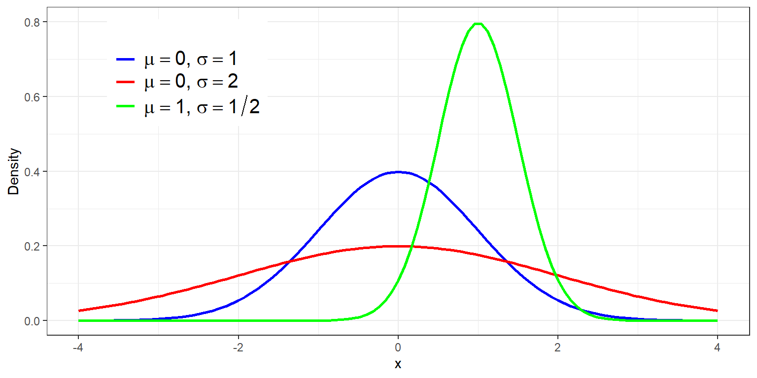
The Normal Distribution
We say that a random variable \(Y\) follows the normal distribution denoted by \(Y\sim Normal(\mu,\sigma^2)\) if and only if the pdf of \(Y\) is given by:
\[ f_Y(y)=\frac{1}{\sqrt{2\pi\sigma^2}}\exp\left\{-\frac{1}{2}\frac{(x-\mu)^2}{\sigma^2}\right\} \]
Remarks:
- If \(Y\sim Normal(\mu,\sigma^2)\) then, \(E(Y)=\mu\), \(Var(Y)=\sigma^2\), \(m_Y(t)=\exp\{\mu t+\frac{1}{2}\sigma^2 t^2\}\)
- The Normal Distribution provides a reasonably good description of the graph of the relative frequency distribution of several random variables.
- A lot of procedures in inferential statistics assume that the population is normally distributed.
- In Stat 136, one of the the most common assumptions is that errors are normally distributed, and expected to be 0.
Results in Sampling from the Normal Distribution
(Sample Mean) Let \(X_1,X_2,...,X_n \overset{iid}{\sim} Normal(\mu,\sigma^2)\) \[ \bar{X}=\frac{1}{n}\sum_{i=1}^n X_i\sim Normal\left(\mu,\frac{\sigma^2}{n}\right) \]
(Sum of Squares of Standard Normal) Let \(Y_1,...,Y_n \overset{iid}{\sim} N(0,1)\). Then \[ \sum_{i=1}^n Y_i^2 \sim \chi^2_{(\nu=n)} \]
(Sample Variance). Let \(S^2\) be the sample variance of \(X_1,X_2,...,X_n\overset{iid}{\sim}N(\mu,\sigma^2)\). Then \[ \frac{(n-1)S^2}{\sigma^2} \sim \chi^2_{(\nu = n-1)} \]
(T Statistic). Let \(Y\sim N(0,1), Z\sim \chi^2_\nu\), \(Y\) and \(Z\) are independent. Then \[ T = \frac{Y}{\sqrt{Z/\nu}} \sim t_{(\nu)} \] Remark: This will be useful in showing that \(\frac{\bar{X}-\mu}{S/\sqrt{n}}\sim t_{(n-1)}\) and \(\frac{\hat{\beta}_j-\beta_j}{\widehat{s.e.(\hat{\beta}_j)}} \sim t_{(n-p)}\)
(F-Statistic). Let \(U\sim\chi^2_{(\nu_1)}, V\sim\chi^2_{(\nu_2)}\), \(U\) and \(V\) are independent. Then \[ F = \frac{U/\nu_1}{V/\nu_2}\sim F(\nu_1,\nu_2) \] Remark: This will be useful in ANOVA outputs in regression.
Point Estimation
Point Estimation uses information in a sample to arrive at a single number that will serve as an estimate of the value of the target parameter.
Important concepts in estimation. Suppose \(T\) is a statistic computed from a sample \(\{X_i\}\)
A statistic \(T\) is a sufficient statistic if the conditional probability function of the sample observations, given \(T\) , does not depend on the parameter \(\theta\). (Also check: Factorization Criterion for Sufficiency)
A statistic \(T\) is said to be complete if and only if \(E(g(T)) = 0\) implies \(g(T)\) is almost surely equal to 0.
It is easy to find complete sufficient statistics when the distribution is a member of exponential family of distributions.
Evaluating estimators. Now, suppose \(\hat{\theta}\) is an estimator for a parameter \(\theta\).
The bias of \(\hat{\theta}\) in estimating \(\theta\) is
\[ Bias_\theta(\hat\theta)=E(\hat{\theta}-\theta) \]
A point estimator \(\hat{\theta}\) is unbiased if \(E (\hat{\theta}) = \theta\).
The variance of the point estimator \(\hat{\theta}\) is given by
\[ Var_\theta(\hat{\theta})=\mathbb{E}\left[\left(\hat{\theta}-\mathbb{E}(\hat{\theta})\right)^2\right] \]
The mean squared error (MSE) of an estimator \(\hat\theta\) in estimating parameter \(\theta\) is given by
\[ MSE_\theta(\hat{\theta})=\mathbb{E}_\theta\left[(\hat{\theta} - \theta)^2\right]=Bias_\theta(\hat{\theta})^2+Var_\theta(\hat{\theta}) \]
If \(\hat{\theta}\) is unbiased, then the MSE is equal to the variance.
Let \(\hat\theta_n=\hat{\theta}(X_1,...,X_n)\) be a sequence of estimators of a parameter \(\theta\) based on a random sample of size \(n\).
The sequence \(\{\hat\theta_n\}\) is said to be
MSE-consistent if and only if
\[ \lim_{n\rightarrow \infty} MSE_\theta(\hat{\theta}_n) = 0\quad \forall \quad \theta \in \Omega \]
That is, bias and variance approach to 0 for large samples.
weakly consistent if and only if
\[ \lim_{n\rightarrow \infty}P(|\hat{\theta}_n-\theta| \geq \varepsilon) = 0 \quad \forall \quad \theta \in \Omega \]
That is, \(\hat{\theta}_n\) converges in probability to \(\theta\).
An estimator \(\hat{θ}\) is said to be uniformly minimum variance unbiased estimator (UMVUE) for \(\theta\) if it has the lowest variance among all unbiased estimators of \(\theta\).
For any other unbiased estimator \(\hat{\theta}'\),
\[ Var(\hat{\theta}) ≤ Var(\hat{\theta}') \]
One of the most popular way of finding the UMVUE is the Lehmann Scheffe Theorem. It states that any unbiased estimator of \(\theta\) which is a function of a complete sufficient statistic is said to be the UMVUE for \(\theta\).
Maximum Likelihood Estimation. The likelihood function generally gives (more or less) the ”likelihood” that the parameter is equal to some value.
- Suppose \(\{X_1,X_2,...,X_n\}\) is a random sample from \(f_X(x|\theta)\). The likelihood function \(L(\theta|x_1,x_2,...,x_n)\) is given by:
\[ L(\theta|x_1,x_2,...,x_n)=\prod_{i=1}^nf_{X_i}(x_i|\theta) \]
an estimator \(\hat{\theta}\) is said to be the maximum likelihood estimator of \(\theta\) if and only if the likelihood function is maximum when \(\theta=\hat{\theta}\).
\[ \hat{\theta}_{MLE} = \underset{\theta}{\arg\max} \{L(\theta|x_1,x_2,...,x_n)\} \]
One of the most popular way of finding the MLE for \(\theta\) is by maximizing the log-likelihood function. This is done by finding the solution to the following equation:
\[ \frac{\partial\ln L(\theta|x_1,...,x_n)}{\partial \theta}=0 \]
Interval Estimation
Interval Estimation uses sample data to calculate the lower and upper bound of an interval such that the researcher can be highly confident that this interval contains the value of the target parameter.
We usually construct a (1 − α)100% confidence interval for the unknown parameter.
The confidence coefficient gives the coverage probability, i.e., the probability that the CI, before sampling, will enclose the true parameter value. Note, however, that once a sample has been observed, a CI ceases to be random and has probability of either 0 or 1 of trapping the true parameter value.
\((1-\alpha)\) is the probability that you will obtain a sample such that if you compute a \((1-\alpha)\) CI, it will capture the parameter, NOT the probability that the parameter is within a specified interval.
The interval is random, the parameter is not.
The most popular way in constructing CIs is the pivotal quantity method. In PQM, you manipulate a pivot, which is a random entity that contains the unknown parameter we are estimating whose distribution is independent of any unknown parameter.
Hypothesis Testing
Hypothesis testing uses sample data to evaluate the validity of a conjecture regarding unknown parameters.
The null hypothesis is the statement being testing; the conjecture the experimenter doubts to be true.
The alternative hypothesis is the operational statement of the theory that the experimenter believes to be true and wished to prove.
Note: The null hypothesis and alternative hypothesis must be non-overlapping statements about the population.
The test statistic is a statistic computed from the sample data that is especially sensitive to the differences between the null and alternative hypotheses.
Note: The test statistic should tend to take on certain values when Ho is true and tend to different values when Ha is true. The decision to reject Ho depends on the value of the test statistic
The region of rejection can be thought of as the set of values of the test of statistic that will lead to the rejection of the null hypothesis.
Errors in Hypothesis Testing:
Type I error: incorrectly rejecting the null when it is true.
Type II error: incorrectly accepting the null when it is false.
Since the Type I error is usually the more drastic of the two errors in hypothesis testing, it is a common approach to set an upper bound to the probability of committing a Type I error (\(\alpha\)), then find the test with the lowest probability of committing a Type II error (\(\beta\)).
Both probability of errors in hypothesis testing can be diminished by increasing the sample size.
The level of significance (\(\alpha\)) is the is the maximum probability of committing a Type I error the researcher is willing to commit.
The power of the test (\(1-\beta\)) is the probability of correctly rejecting the null hypothesis
The power function \(K_\phi(\theta)\) gives the probability of rejecting the null hypothesis based on a value of the parameter.
Likelihood Ratio Test
- One of the most popular way in creating a test is the likelihood ratio test which depends on the test statistic \(\lambda\) given by \[ \lambda = \frac{\underset{\Omega_0}{\sup}\mathcal{L}(\theta,\textbf{X})}{\underset{\Omega}{\sup}\mathcal{L}(\theta,\textbf{X})} \]
- The asymptotic distribution under \(Ho\) of the test statistic \(-2\ln(\lambda)\) is given by \(\chi^2_{(\nu)}\), where \(\nu\) is the number of unknown parameters on the parameter space minus the number of unknown parameters under the null hypothesis.
0.3 Measures of Correlation
What is a Correlation Coefficient?
Measures the degree of association of 2.
The value is usually between -1 and +1.
Any value close to +1 implies strong direct relationship while a value close to -1 implies strong inverse relationship. A value close to 0 implies weak or no relationship.
The coefficient does not imply structural relationship and does not indicate causality between the variables.
Although different, correlational analysis is oftentimes done as a preliminary step to explore data before doing regression analysis. There are many types of correlation coefficient. Few are summarized here.
Pearson’s \(r\)
The Pearson product-moment correlation coefficient measures the correlation between two continuous variables. This coefficient may underestimate the degree of association if relationship is nonlinear.
\[ r = \frac{\sum_{i=1}^n(x_i-\bar{x})(y_i-\bar{y})}{\sqrt{(\sum_{i=1}^n(x_i-\bar{x})^2)(\sum_{i=1}^n(y_i-\bar{y})^2)}} \]
Example
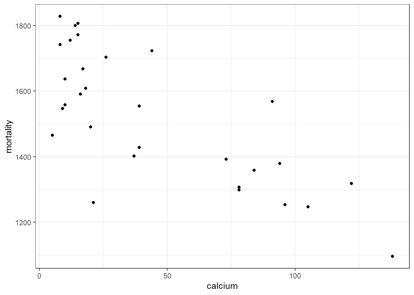
A sample of 30 towns were drawn and mortality rate and calcium concentrating in drinking water were determined.
- \(Y\) = 7-year mortality rate (per 100,000)
- \(X\) = average calcium ion concentration in drinking water (ppm)
| mortality | calcium |
|---|---|
| 1247 | 105 |
| 1800 | 14 |
| 1807 | 15 |
| 1359 | 84 |
| 1307 | 78 |
| 1555 | 39 |
| 1260 | 21 |
| 1742 | 8 |
| 1569 | 91 |
| 1772 | 15 |
| 1668 | 17 |
| 1609 | 18 |
| 1299 | 78 |
| 1392 | 73 |
| 1254 | 96 |
| 1428 | 39 |
| 1723 | 44 |
| 1547 | 9 |
| 1591 | 16 |
| 1828 | 8 |
| 1466 | 5 |
| 1558 | 10 |
| 1637 | 10 |
| 1755 | 12 |
| 1491 | 20 |
| 1318 | 122 |
| 1379 | 94 |
| 1096 | 138 |
| 1402 | 37 |
| 1704 | 26 |
##
##  Pearson's product-moment correlation
##
## data:  calcium$mortality and calcium$calcium
## t = -6.0649, df = 28, p-value = 1.537e-06
## alternative hypothesis: true correlation is not equal to 0
## 95 percent confidence interval:
##  -0.8759845 -0.5397840
## sample estimates:
##        cor
## -0.7535183
Conclusion: Reject the hypothesis that there is no correlation.
The data indicates that there is a strong inverse relationship between mortality and calcium level in drinking water.
Spearman’s \(\rho\)
The Spearman Rank Correlation is a measure of correlation of rankings. The variables were both measured at least in an ordinal scale.
\[
\rho = \frac{6 \sum d_i^2}{n (n^2-1)}
\]
where \(d_i\) is the difference between ranks of two variables of observation \(i\)
Example
Ten materials for artificial reef were evaluated.
- \(Y\) = ranking according to number of invertebrates attracted after 1 month.
- \(X\) = ranking according to cost and availability of materials.
| Material | X | Y |
|---|---|---|
| 1 | 1 | 3 |
| 2 | 4 | 2 |
| 3 | 2 | 4 |
| 4 | 3 | 5 |
| 5 | 5 | 1 |
| 6 | 6 | 7 |
| 7 | 7 | 8 |
| 8 | 8 | 6 |
| 9 | 9 | 9 |
| 10 | 10 | 10 |
##
##  Spearman's rank correlation rho
##
## data:  reef$X and reef$Y
## S = 38, p-value = 0.01367
## alternative hypothesis: true rho is not equal to 0
## sample estimates:
##      rho
## 0.769697
Kendall’s \(\tau\)
The Kendall Rank correlation coefficient coefficient is also used to measure the ordinal association between two measured quantities.
\[\begin{align} \tau &= \frac{(\text{number of concordant pairs}-\text{number of discordant pairs})}{\text{number of pairs}} \\ &= 1-\frac{2(\text{number of discordant pairs})}{n\choose 2} \end{align}\]
Example
We use the sample example in the Spearman Correlation:
- \(Y\) = ranking according to number of invertebrates attracted after 1 month.
- \(X\) = ranking according to cost and availability of materials.
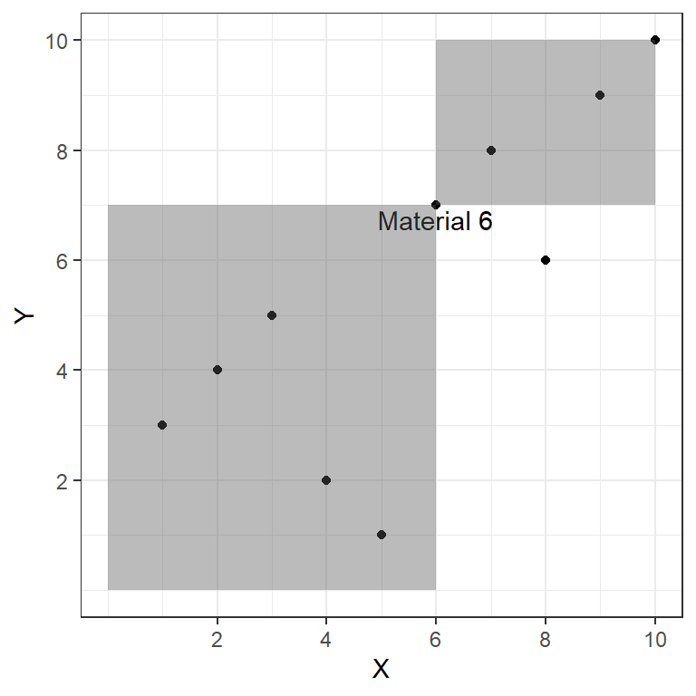
With respect to Material 6, there is only one material that is discordant to it, while the other eight are concordant to it.
##
##  Kendall's rank correlation tau
##
## data:  reef$X and reef$Y
## T = 36, p-value = 0.01667
## alternative hypothesis: true tau is not equal to 0
## sample estimates:
## tau
## 0.6
The 3 correlation coefficients above are the most common coefficients, especially the Pearson’s r for numeric and continuous variables. The Kendall’s Tau and Spearman’s Rho cannot be used directly for continuous variables, unless they are converted to ranks.
The following coefficients measure association of categorical variables.\(\phi\) Coefficient
The Phi Coefficient is used if both variables are dichotomous.
| X | 0 | 1 |
| 0 | a | b |
| 1 | c | d |
\[ \phi=\frac{|ad-bc|}{\sqrt{(a+b)(c+d)(a+c)(b+d)}} \]
Contingency Coefficient
Used if variables are both categorical.
| X | category 1 | category 2 | category 3 |
| category 1 | a | d | g |
| category 2 | b | e | h |
| category 3 | c | f | i |
\[ C = \sqrt{\frac{\chi^2}{n+\chi^2}} \] where \(\chi^2\) is the chi-squared test statistic which can be computed using the contingency table.
Other measures of association if at least one is categorical
- Biserial - one variable is continuous vs. another continuous variable which has been artificially dichotomized.
- Point-biserial - one continuous vs. another which is a true dichotomy; conservative, and more applicable and safe to use when in doubt.
- Tetrachoric - both variables are quantitative and both have been artificially dichotomized.
- Eta-coefficient - one variable is interval and one is nominal.
0.4 Review Questions
Show Questions
True or False
The unbiased estimator that is a function of a sufficient statistic is the UMVUE.
A square \(\textbf{J}\) matrix is always full rank.
If the bias of an estimator approaches 0 for large samples, then it is MSE consistent.
The ratio of two Chi-square random variables is an \(F\) random variable.
If \(X_1,...,X_n\) are independent Normal random variables, then the linear combination of these variables \(\sum_{i=1}^n(a_iX_i+b_i)\) is also Normally distributed, where \(\{a_n\}\) and \(\{b_n\}\) are sequences of constants.
Suppose \(X_1,X_2,...,X_n\overset{iid}{\sim}N(\mu,\sigma^2)\). The MLE for \(\mu\) is \(\bar{X}\)
If two random variables are independent, then they are uncorrelated.
If two random variables are uncorrelated, then they are independent.
The covariance matrix is always symmetric.
As the sample size increases, the standard error of the sample mean decreases.
The centering matrix \(\textbf{C}\) is symmetric and idempotent.
Suppose \(\textbf{X}\) is an orthogonal matrix of dimension 5. Then the rank of \(\textbf{XX}'\) is 5.
Suppose \(\textbf{X}\) is an \(n\times p\) matrix. The rank of \(\textbf{X}'\textbf{X}\) is \(p\).
If \(f(\textbf{x})=\textbf{x}'\textbf{Ax}\), where \(\textbf{x}\) is an \(n\times1\) vector and \(\textbf{A}\) is an \(n\times n\) symmetric matrix, then \(\frac{\partial f(\textbf{x})}{\partial \textbf{x}}=2\textbf{A}\textbf{x}\)
When \(Var(T)\rightarrow0\) as \(n\rightarrow \infty\), then \(T\) is a consistent estimator.
Show Answers
False. The unbiased estimator must be a function of the complete sufficient statistic.
False.
False. Variance must also approach 0.
False. Must be independent.
True.
True.
True
False. Only if normally distributed.
True.
True.
True.
True. \(\textbf{XX}'=\textbf{I}_5\)
False. Only true of \(\textbf{X}\) is full rank.
True.
False. Consistent around its own mean, but not in estimating a specific parameter. Bias should also approach 0.