CHAPTER 9 Assessing General Diagnostic Plots and Testing for Linearity

When doing regression analysis, the possible model pitfalls are:

The regression function is not linear. (Nonlinearity, Chapter 9)
Error terms are not normally distributed. (Nonnormality, Chapter 10 )
Error terms do not have constant variance. (Heteroskecasticity, Chapter 10)
Error terms are not independent. (Autocorrelation, Chapter 11)
There is linear dependency among the set of regressors. (Multicollinearity, Chapter 12)
Model fits all but one or few observations (Existence of Outliers and Influential Observations, Chapter 13).

Note: having no outliers or influential observations in the dataset is not a model assumption, however, it may affect the model fit in general.

Chapters 9 to 13 will focus on diagnostic checking of regression assumptions.

In this chapter, we explore how to assess general diagnostic plots such as Residual Plots, Partial Regression Plots, and Residual Plots. However, graphs can also be used for several other purposes:

Explore relationships among variables.
Confirm or negate assumptions.
Assess the adequacy of a fitted model.
Detect outlying observations in the data.
Suggest remedial actions (e.g., transform the data, redesign the experiment, collect more data, etc.).

The assumption of linearity is also checked. If the linearity assumption is not met, some remedial measures are also suggested here.

Most of the diagnostics will be performed using the olsrr package in R.

Full manual of the regression diagnostics using this package can be found here: https://cran.r-project.org/web/packages/olsrr/vignettes/regression_diagnostics.html

9.1 Residual Plots

Recall: The residuals of the fitted model is \[\begin{align} \textbf{e} & = \textbf{Y} − \hat{\textbf{Y}}=\textbf{Y} − \textbf{X}\hat{\boldsymbol{\beta}} \\ &= (\textbf{I}-\textbf{X}(\textbf{X}'\textbf{X} )^{−1}\textbf{X}')\textbf{Y}\\ &= (\textbf{I} − \textbf{H})\textbf{Y} \end{align}\] Review definition and remarks about the residuals in Definition 4.3

Remarks:

The residuals is not exactly the error term, but departures from the assumptions of the error terms will likely reflect on the residuals.
To validate assumptions on the error terms, we will validate the assumptions on the residuals instead.
After we have examined the residuals, we shall be able to conclude either
1. the assumptions appear to be violated, or
2. the assumptions do not appear to be violated.
Concluding (2) does not mean that we are concluding that the assumptions are correct; it means merely that, on the basis of the data we have seen, we have no reason to say that they are incorrect.

Theorem 9.1 (Variance and Covariances of the Residuals)

\(Var(\textbf{e})=\sigma^2(\textbf{I}-\textbf{H})\)
\(Var(e_i)=\sigma^2(1-h_{ii})\) where \(h_{ii}\) is the \(i^{th}\) diagonal element of \(\textbf{H}\) (usually called the leverage)
\(Cov(e_i,e_j)=-\sigma^2h_{ij}\)
\(\rho(e_i,e_j)=-\frac{h_{ij}}{\sqrt{(1-h_{ii})(1-h_{jj})}}\)

Remarks:

Unlike the error terms \(\varepsilon_i\) residuals are not independent to each other and correlation exists among them.
When the sample size is large in comparison to \(p\), this dependence of the residuals has little effect on their use for checking model adequacy.
The effect is usually negligible. The residuals will be used in validating the assumptions. A simple method of doing this is by looking at the residual plots.

Definition 9.1 (Residual Plot) A residual plot is a scatter plot of the residuals (plotted on the vertical axis of the Cartesian plane) and other elements of regression modelling such as fitted values of Y and values of the regressors \(X_j\) (plotted on the horizontal axis).

Why do we plot the residuals against the fitted values and the values of the regressors and NOT against the observed response values for the usual linear model?

If the model follows all the assumptions, the residuals and the response values are usually correlated.
But the residuals and regressors and fitted values are not.
- Theorem 4.9: \(Cov(e_i,X_{ji})=0\)
- Theorem 4.10: \(Cov(e_i,\hat{Y})=0\)
One of our goals in looking at residual plots is to check whether there are patterns in the plot itself.
- Since the response values and residuals are usually correlated, this relationship will affect the interpretation of the plot, and expected to have some pattern.
- On the other hand, if there is a recognizable pattern in the residuals vs fitted plot or the residuals vs regressors plot, then there might be something wrong in the model.

Exercise 9.1 Show the following:

correlation of the residuals \(e_i\) and the dependent variables \(Y_i\) is equal to \(\sqrt{1-R^2}\)
correlation of the residuals \(e_i\) and the fitted values \(\hat{Y}_i\) is equal to 0

Interpretation of Residual Plots

The following are prototypes of residual plots:

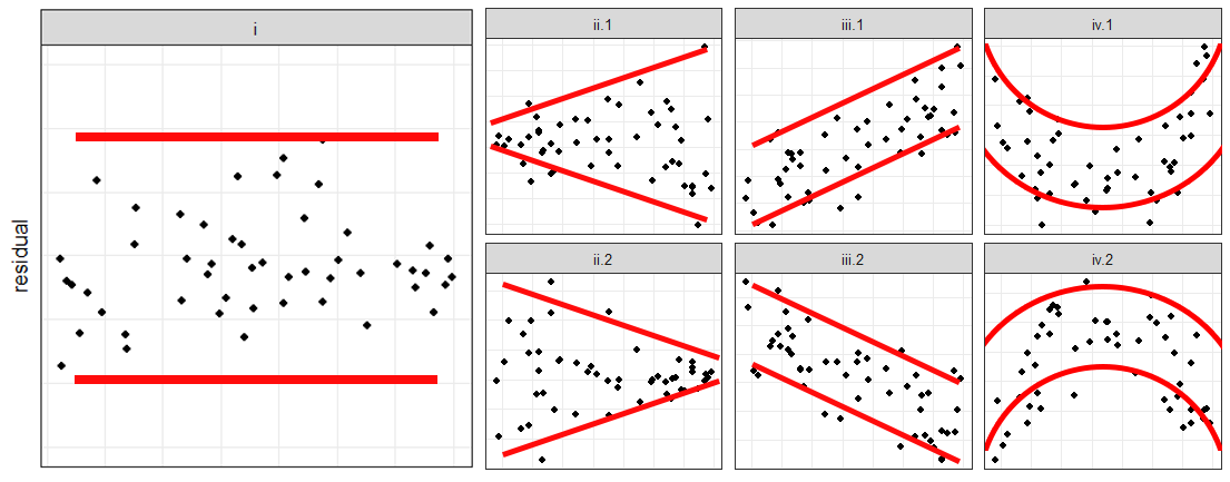
If \(\hat{Y}\) is in the horizontal axis
1. No irregularity indicated since the residuals are contained in a horizontal band
2. Variance is not constant - there is a need to do weighted least squares or a transformation on the \(Y_i\)s.
3. Error in analysis - there is a systematic departure from fitted equation. This may be due to wrongly omitting \(\beta_0\) from the model.
4. The model is inadequate or the model is nonlinear - need extra terms or other regressor/independent variables or cross-product terms, or need for a transformation on the \(Y_i\)s before analysis.
One of the \(X\)s is on the horizontal axis
1. No irregularity
2. Variance is not constant - there is a need to do weighted least squares or a preliminary transformation on the \(Y_i\)s.
3. Error in calculation - linear effect of \(X_j\) not removed. This could probably occur if the problem of multicollinearity is present.
4. Need for extra terms - e.g. a quadratic term in \(X\) or a transformation on the \(Y_i\)s.

Illustration in R:

The resid() function extracts the residuals, and the fitted() function extracts the fitted values from an lm object in R

mod_anscombe <- lm(income~young+urban+education, data = Anscombe)
plot(fitted(mod_anscombe),resid(mod_anscombe))

For customization, you can use ggplot.

data.frame(resid = resid(mod_anscombe), 
           fitted.income = fitted(mod_anscombe),
           young = Anscombe$young,
           urban = Anscombe$urban,
           education = Anscombe$education) |> 
    pivot_longer(cols = c(fitted.income,young,urban,education)) |>
    mutate(name = factor(name, levels = c("fitted.income","education", "urban", "young"))) |> 
    ggplot(aes(y = resid, x = value))+
    geom_point()+
    facet_grid(.~name, scales = 'free_x') + theme_bw() + xlab("") + ylab("residual")

olsrr package also have tools for plotting residual plots.

Residual vs Fitted
```
olsrr::ols_plot_resid_fit(mod_anscombe)
```

Residual vs Regressors

olsrr::ols_plot_resid_regressor(mod_anscombe, 'young', print_plot = F)

olsrr::ols_plot_resid_regressor(mod_anscombe, 'urban', print_plot = F)

olsrr::ols_plot_resid_regressor(mod_anscombe, 'education', print_plot = F)

Partial Regression Plot

Definition 9.2 Consider a linear regression model with k independent variables \(X_1, X_2, ..., X_k\). The plot of the residuals obtained after regressing \(Y\) on all the \(Xs\) except \(X_j\) and the residuals obtained after regressing \(X_j\) on the other \(Xs\) is called the partial regression plot of \(Y\) against \(X_j\).

Plots of this kind are also called added variable plots, partial regression leverage plots, or simply partial plots.
The partial regression plot presents the marginal relationship between the response and the predictor after the effect of the other predictors has been removed.
The partial regression plot allows us to focus on the relationship between one predictor and the response, much as in simple regression.
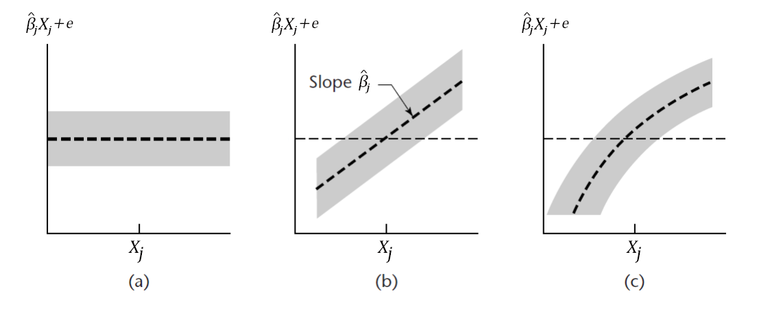
The following are the prototypes for the added-variable plot.

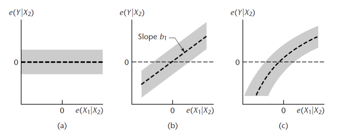
Interpretation:
1. There is no more unique information from \(X_1\) when \(X_2\) is already in the model.
2. There is still a unique linear information from \(X_1\) when \(X_2\) is already in the model.
3. There is still a unique nonlinear information from \(X_1\) when \(X_2\) is already in the model.
Limitations: A common remedial measure for nonlinearity is transformation of variables. The partial regression plot may give misleading information of the proper way to transform variables as the plot adjusts \(X_j\) for the other \(X\)s, but it is the unadjusted \(X_j\) that is transformed in re-specifying the model.

Illustration in R:

ols_plot_added_variable() from olsrr package.

olsrr::ols_plot_added_variable(mod_anscombe)

avPlots() function from the car package
```
car::avPlots(mod_anscombe)
```

Partial Residual Plot

Definition 9.3 Consider the estimated regression function given by \(\hat{Y}=\hat{\beta_0}+\hat{\beta_1}X_1+\hat{\beta}_2X_2+\cdots+\hat{\beta}_kX_k\) and the residual \(e_i = Y_i-\widehat{Y}_i\)

Then \(Y_i^{(j)} = e_i + \hat{\beta}_j X_{ij}\) is the “partial residuals” or the “residual plus component”, which is \(Y_i\) with the linear effects of the other variables removed.

The plot of \(Y^{(j)}\) against \(X_j\) is called a partial residual plot.

This is also called a component plus residual plot.
The interpretation of partial residual plot is also like that of partial regression plots.
The partial residual plot is often an effective alternative to partial regression plot. This is because we plot ”untranslated \(X\)s” it is easier to verify appropriate transformations for \(X\)s.

Limitation: For finding outliers and influential observations, however, the partial residual plot is not as suitable as the partial regression plot.

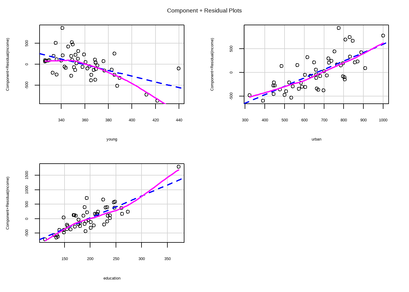
Illustration in R:

ols_plot_comp_plus_resid() from the olsrr package
```
olsrr::ols_plot_comp_plus_resid(mod_anscombe)
```
crPlot() from the car package, but the Y axis is centered around 0. Suggested transformations can also be seen.
```
car::crPlots(mod_anscombe)
```

More of these will be discussed later in detecting nonlinearity.

Exercise 9.2 Load the mtcars dataset using data("mtcars"). Create a linear model with mpg as the dependent variable, and the disp, ht, wt, and qsec as independent variables.

Create the following plots:

Regular Scatter plot of the Independent Variables vs Dependent Variable (4 scatterplots)
Regressor vs Residual Plots
Fitted vs Residual Plot
Partial Regression Plots
Partial Residual Plots

Give short comments about the plots.

9.2 On Nonlinearity

Definition 9.4 Nonlinearity is the case wherein the mean of \(Y\) is not linearly related with at least one of the regressors. That is, \[ E (Y) \neq \beta_0 + \beta_1X_1 + \cdots + \beta_kX_k \]

The usual reasons for nonlinearity are:

The relationship between the response and the regressors are inherently nonlinear. For instance, a partial relationship specified to be linear may be quadratic, logarithmic, exponential, etc…, or two independent variables do not have additive partial effects in \(Y\).
Exclusion of very important predictor variables

Implications of Nonlinearity

The assumption that the regression equation is \(E(Y) = \beta_0 + \beta_1X_1 + \cdots + \beta_k X_k\) implies that the specified linear regression model captures the dependency of \(Y\) on the \(X\)’s. Violating the assumption of linearity therefore implies that the model fails to capture the linear systematic pattern of relationship between the dependent and independent variables.
The fitted model is frequently a useful approximation even if \(E(Y)\) is not precisely captured. In other cases, however, the model can be extremely misleading.
The problem of nonlinearity, if not resolved, can oftentimes affect the adequacy of the model in fitting the data at hand, giving bad fit as evidenced by low R-squared or nonsignificant regressors.
The problem of nonlinearity can also cause gross violations in the model assumptions such as nonnormality and heteroskedasticity.
Because of this, it is oftentimes suggested by many statisticians to resolve the problem of nonlinearity first before solving other possible model pitfalls.

Graphical Tools for Detecting Nonlinearity

Here are some of the graphical tools we can use to check whether the model satisfies the linearity assumption:

Regular Scatter Plot

Creating a scatter plot of each of the X ’s and the Y is a usual preliminary step to check whether individual X ’s are linearly related with Y .

Limitations:

It doesn’t take into account the marginal relationship of Y with the X ’s when all other variables are already in the model. We are much more interested with this as in regression, we hope that all the regressors are helping in explaining Y .
It doesn’t take into account the relationship of regressors with one another.

Regressor vs Residual Plot

Another plot that we can use is the usual regressor vs residual plot. We can say that the model is nonlinear if the residuals depart from 0 in a systematic fashion.

Limitations:

The residual plots cannot distinguish between monotone and non-monotone nonlinearity. The distinction is lost in the residual plots because the least squares fit ensures that the residuals are linearly uncorrelated with each X .
This distinction is important because monotone nonlinearity frequently can be corrected by simple transformations.

Partial Regression Plot

Added variable plot provides information about the marginal importance of a predictor variable \((X_{j})\), given the other predictor variables already in the model. It shows the marginal importance of the variable in reducing the residual variability.

A strong linear relationship in the added variable plot indicates the increased importance of the contribution of X to the model already containing the other predictors. In other words, we can say that the variable gives a unique linear information to the model if the plot looks like a straight (diagonal) line.

Partial Residual Plot

The residual plus component plot indicates whether any non-linearity is present in the relationship between Y and X and can suggest possible transformations for linearizing the data.

Testing for Nonlinearity

We can do a formal test for determining whether or not a specified linear regression model adequately fits the data.

We will quickly introduce the following hypotheses tests that are related to linearity.

The Classic Lack of Fit Test

The classic lack-of-fit test require repeat observations at one or more X levels.

Definition 9.5 (Replication and Replicates) Repeated trials for the same levels of the independent variables are called replications and the resulting observations are called replicates.

In the Lack of Fit Test, we further decompose the SSE into two components: Sum of Squares due to Pure Error (SSPE) and Sum of Squares due to Lack of Fit (SSLF).

Pure Error - deviations attributed due to replications at some levels of X , deviations attributed to random variation of the data
Lack-of-Fit - deviation of fitted value from mean of Y at a given X level

Let \(Y_{im}\) denote the \(i^{th}\) observation for the \(m^{th}\) level of \(\textbf{x}\) (whether there is replication or none) where \(i = 1, 2, . . . , n_m\) and \(m = 1, 2, . . . , c\).

Source of Variation	Sum of Squares	df	Mean Square	F
Regression	SSR	p-1	MSR	\(F_2=\frac{MSR}{MSE}\)
Error	SSE	n-p	MSE
Lack of Fit	SSLF	c-p	MSLF	\(F_1=\frac{MSLF}{MSPE}\)
Pure Error	SSPE	n-c	MSPE
Total	SST	n-1

where

\(SSE = SSLF+SSPF\)
\(SSPE=\sum_{m=1}^c\sum_{i=1}^{n_m}(Y_{im}-\bar{Y}_m)^2\)
\(MSLF=\frac{SSLF}{c-p}\)
\(MSPE=\frac{SSPE}{n-c}\)
Critical Region: Reject Ho if \(F_1>F_{\alpha, (c-p) , (n-c) }\)

Simple Illustration:

Limitations:

The test needs replication in X . This is hard to establish when the values of the X ’s are not predetermined. This is not a problem in experimental designs.
Certain modifications of the test has been proposed for this limitation. Daniel and Woods (1980) has proposed the concept of ”near replicates” to establish replications. More solutions has been proposed by Joglekar et. al. (1989).
The test requires that the model follows the normality and homoskedasticity assumption.

The Ramsay’s RESET

Definition 9.6 The Ramsey’s Regression Specification Error Test (RESET) tests whether non-linear combinations of the explanatory variables help to explain the response variable.

Idea: If a regression is specified appropriately you should not be able to find additional independent variables. To test this, the RESET regresses the dependent variable against the polynomial of the fitted values and the original variables, fitting the following model:

\[ Y=a_0+b_1X_1+\cdots+b_kX_k+c_1\hat{Y}^2+\cdots+c_{k-1}\hat{Y}^k+\varepsilon \]
The F-test is conducted comparing the model above with the original model (same philosophy as the General Linear Test).
Limitation: Low power in detecting nonlinearity
Advantage: The test does not require replication

The Harvey-Collier Test

This test makes use of the recursive residuals which are linear transformations of the ordinary residuals.

Prior to testing, you need to order the sample from lowest to highest in terms of the regressor variable.
The recursive residuals are given by:

\[ u_j=\frac{e_j}{\sqrt{1+\textbf{x}_j'(\textbf{X}_j'\textbf{X}_j)^{-1}\textbf{x}_j}} \]

where \(e_j\) is the \(j^{th}\) residual from the first \(j\) observations, \(\textbf{x}_j\) is the \(j^{th}\) observation vector, and \(\textbf{X}_j\) is the design matrix involving the first \(j\) observations.
If the model is correctly specified, recursive residuals have mean zero. If mean differs from zero, ordering variable has an influence on the regression relationship.
Simple t-test is used for the recursive residuals.

Limitations:

This test is only powerful when only one regressor is misspecified.
This test is also only powerful for nonlinearity wherein the relationship forms a concave or a convex.

Advantages:

This test is robust to nonnormality and autocorrelation problem
This test does not need replications.

The Rainbow Test

Idea: Even a misspecified model might fit (reasonably) well in the “center” of the sample but might lack fit in the tails.
Fit model to a subsample (typically, the middle 50%) and compare with full sample fit using an F test (same philosophy as the General Linear Test).
With this, you also need to order the observations by the response or the regressor.
Limitation: This test is only powerful for nonlinearity wherein the relationship forms a concave or a convex.
Advantage: This test does not need replications.

Remedial Measures: Transformations

Simple transformations of either the response variable Y or the predictor variables X , or of both, are often sufficient to make the linear regression model appropriate for the data with problem of nonlinearity.

Note: A model is linear if parameters \(\beta\) appear as linear components, regardless of the complexity (nonlinearity) of the predictor variables.

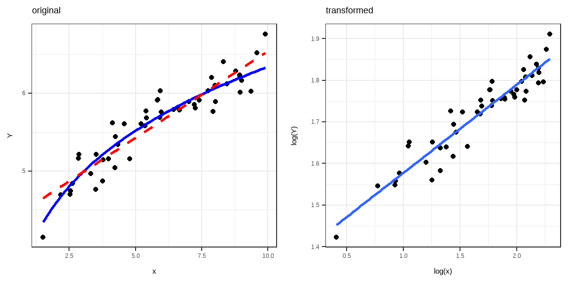
The following are examples of nonlinear relationships between the X and Y variables. The red dashed line is the fitted line if we assume that X and Y are linearly related.

Function: \(Y=aX^\beta\) Transformations: \(Y^*=\log(Y), X^*=\log(X)\)

Linear form: \(Y^*=\log(a)+\beta X^*\)
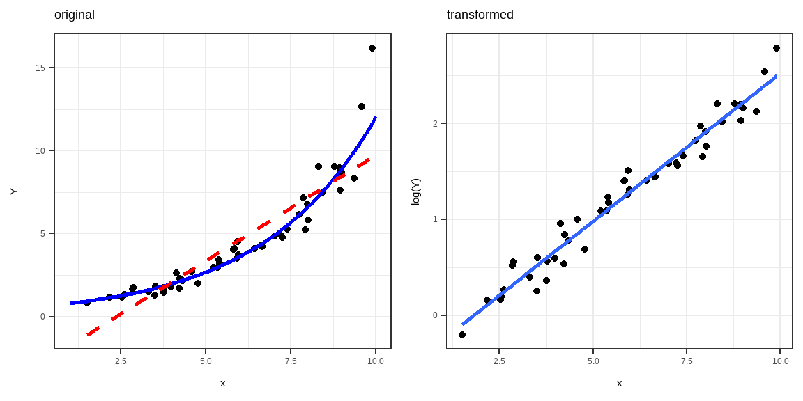
Function: \(Y=ae^{\beta x}\) , Transformation: \(Y^*=\log(Y)\) , Linear Form: \(Y^*=\log(a)+\beta X\)
Function: \(Y=a+\beta\log (X)\) Transformation: \(X^*=\log(X)\) Linear Form: \(Y=a+\beta X^*\)
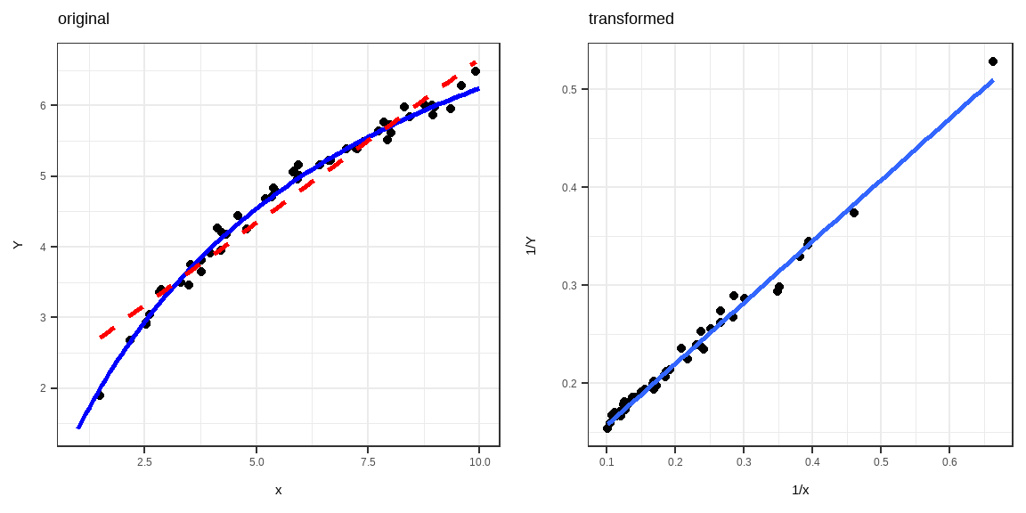
Function: \(Y=\frac{X}{aX-\beta}\), Transformation: \(Y^*=\frac{1}{Y},\quad X^*=\frac{1}{X}\), Linear Form: \(Y^*=a-\beta X^*\)
Function: \(Y=\frac{\exp(a+\beta X)}{1+\exp(a+\beta x)}\) Transformation: \(Y^*=\log(\frac{Y}{1-Y})\)

Linear Form: \(Y^*=a+\beta X\)

Remarks on transformations:

If non-linearity is an issue, use a scatter plot to find helpful transformations.
- This only works for simple linear regression (one predictor).
- For multiple linear regression, analyze residual plots instead.
Transformations should be based on sound theory, reason, and logic.
- Use related literature in justifying the transformation you are going to use.
- Do not hastily use a transformation just because the results improved.
Take note of the range of your data and the support of the function that you are going to use.
- For example, applying the \(\log(\cdot)\) function on a variable with 0 or negative values may pose some errors.
It is recommended to transform the \(Xs\) first before you decide to transform \(Y\).
- Interpretation of the expectation may be different if you transform \(Y\).
- Note that for a function \(g(\cdot)\), \(E(g(X))\neq g(E(X))\).
- That is, the expected value of a transformation of \(Y\) is not the same as the transformation of the expected value of \(Y\).
Some transformations may cause heteroskedasticity or violation of other assumptions. Do not forget to check residual variance and diagnostic plots again every after transformation.

References

- Hebbali, A. (2017). olsrr: Tools for Building OLS Regression Models [Dataset]. https://doi.org/10.32614/cran.package.olsrr