Chapter 1 Preliminaries
This chapter provides new important concepts and a little overview that will be useful in linear regression and model building.
1.1 Overview of Regression
Definition 1.1 Regression analysis is a statistical tool which utilizes the relation between two or more quantitative variables so that one variable can be predicted from the other(s).
The main objective of the analysis is to extract structural relationships among variables within a system. It is of interest to examine the effects that some variables exert (or appear to exert) on other variable(s).
Linear regression is used for a special class of relationships, namely, those that can be described by straight lines. The term simple linear regression refers to the case wherein only two variables are involved; otherwise, it is known as multiple linear regression.
Visualization
A good way to start regression analysis is by plotting one variable against another in a scatter plot.
This helps reveal their relationship and highlights any potential issues. The graph indicates the general tendency by which one variable varies with changes in another variable.
The scatter plot only is useful in the simple linear regression case.
| PRICE | TAX |
|---|---|
| 53 | 652 |
| 55 | 1000 |
| 56 | 897 |
| 58 | 964 |
| 64 | 1099 |
| 44 | 960 |
| 49 | 678 |
| 72 | 800 |
| 82 | 1038 |
| 85 | 1200 |
| 45 | 860 |
| 47 | 600 |
| 49 | 676 |
| 56 | 1287 |
| 60 | 834 |
| 62 | 734 |
| 64 | 551 |
| 66 | 1355 |
| 35 | 561 |
| 38 | 489 |
| 43 | 752 |
| 46 | 774 |
| 46 | 440 |
| 50 | 549 |
| 65 | 900 |
## [1] 0.5774705##
## Call:
## lm(formula = PRICE ~ TAX, data = house)
##
## Coefficients:
## (Intercept) TAX
## 31.39144 0.02931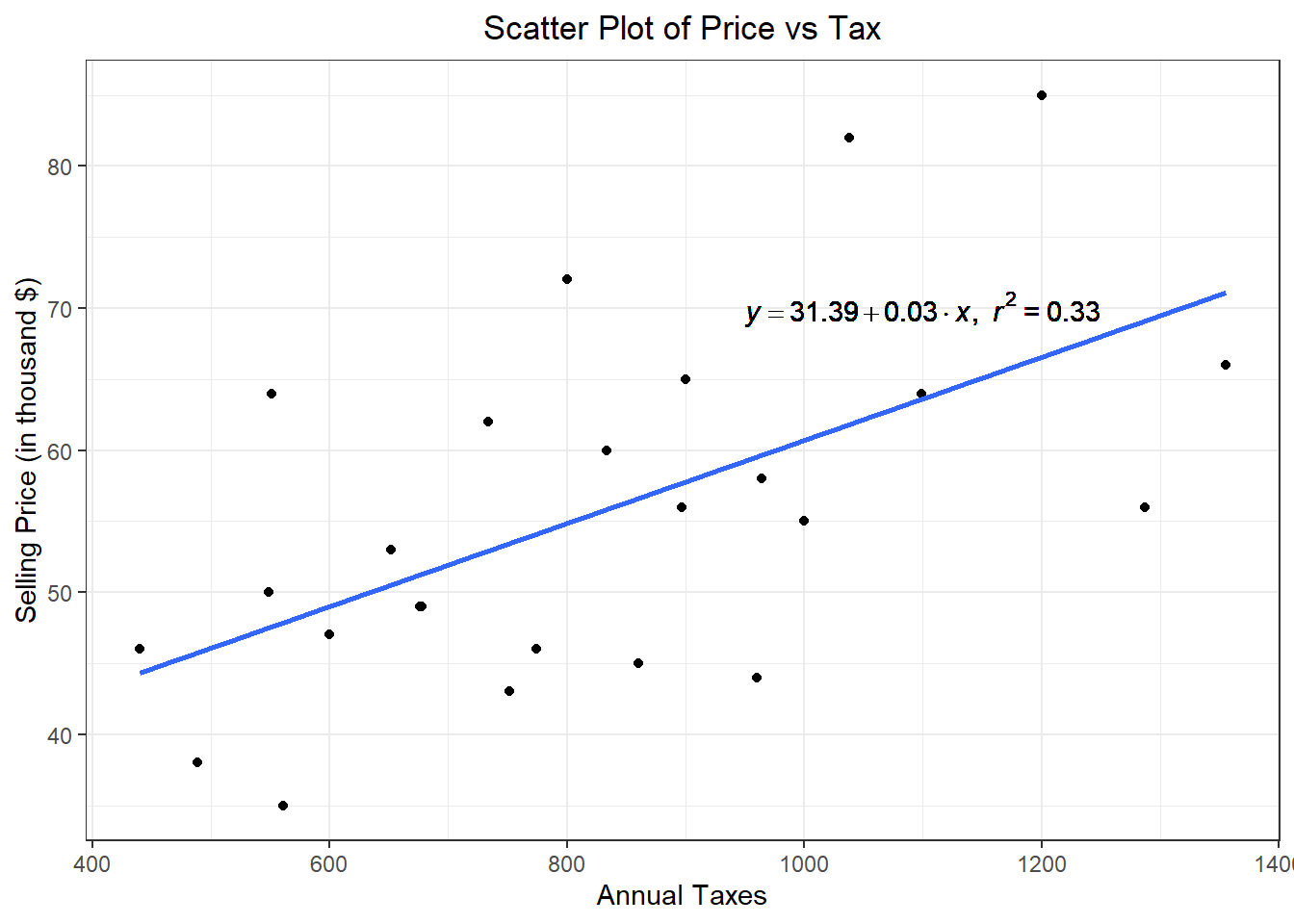
1.2 The Model Building Process
WHAT ARE MODELS?
Model is a set of assumptions that summarizes the structure of a system.
Types of Models
Deterministic Models: models that produce the same exact result for a particular set of input.
Example: income for a day as a function of items sold.
Stochastic Models: models that describe the unpredictable variation of the outcomes of a random experiment.
Example: Grade of Stat 136 students using their Stat 131 grades. Take note that Stat 136 grades may still vary due to other random factors.
In Statistics, we are focused on Stochastic Models.
Types of Variables in a Regression Problem
dependent (regressand, endogenous, target, output, response variable) - whose variability is being studied or explained within the system.
independent (regressor, exogenous, feature, input, explanatory variable) - used to explain the behavior of the dependent variable. The variability of this variable is explained outside of the system.
Examples
Can we predict a selling price of a house from certain characteristics of the house? (Sen and Srivastava, Regression Analysis)
dependent variable - price of the house
independent variables - number of bedrooms, floor space, garage size, etc.Is a person’s brain size and body size predictive of his or her intelligence? (Willerman et al., 1991)
dependent variable - IQ level
independent variables - brain size based on MRI scans, height, and weight of a person.What are the variables that affect the total expenditure of Filipino households based on the Family Income and Expenditure Survey (PSA, 2012)?
dependent variable - total annual expenditure of the households
independent variables - total household income, whether the household is agricultural, total number of household membersWhat are the determinants of a movie’s box-office performance? (Scott, 2019)
dependent variable - box office figure
independent variables - production budget, marketing budget, critical reception, genre of the movie
Types of Data
Time-series data - a set of observations on the values that a variable takes at different times (example: daily, weekly, monthly, quarterly, annually, etc.)
Date Passengers 1949-01-01 112 1949-01-31 118 1949-03-02 132 1949-04-02 129 1949-05-02 121 1949-06-02 135 1949-07-02 148 1949-08-01 148 1949-09-01 136 1949-10-01 119 1949-11-01 104 1949-12-01 118 1950-01-01 115 1950-01-31 126 1950-03-02 141 1950-04-02 135 1950-05-02 125 1950-06-02 149 1950-07-02 170 1950-08-01 170 1950-09-01 158 1950-10-01 133 1950-11-01 114 1950-12-01 140 1951-01-01 145 1951-01-31 150 1951-03-02 178 1951-04-02 163 1951-05-02 172 1951-06-02 178 1951-07-02 199 1951-08-01 199 1951-09-01 184 1951-10-01 162 1951-11-01 146 1951-12-01 166 1952-01-01 171 1952-01-31 180 1952-03-02 193 1952-04-01 181 1952-05-02 183 1952-06-01 218 1952-07-02 230 1952-08-01 242 1952-09-01 209 1952-10-01 191 1952-11-01 172 1952-12-01 194 1953-01-01 196 1953-01-31 196 1953-03-02 236 1953-04-02 235 1953-05-02 229 1953-06-02 243 1953-07-02 264 1953-08-01 272 1953-09-01 237 1953-10-01 211 1953-11-01 180 1953-12-01 201 1954-01-01 204 1954-01-31 188 1954-03-02 235 1954-04-02 227 1954-05-02 234 1954-06-02 264 1954-07-02 302 1954-08-01 293 1954-09-01 259 1954-10-01 229 1954-11-01 203 1954-12-01 229 1955-01-01 242 1955-01-31 233 1955-03-02 267 1955-04-02 269 1955-05-02 270 1955-06-02 315 1955-07-02 364 1955-08-01 347 1955-09-01 312 1955-10-01 274 1955-11-01 237 1955-12-01 278 1956-01-01 284 1956-01-31 277 1956-03-02 317 1956-04-01 313 1956-05-02 318 1956-06-01 374 1956-07-02 413 1956-08-01 405 1956-09-01 355 1956-10-01 306 1956-11-01 271 1956-12-01 306 1957-01-01 315 1957-01-31 301 1957-03-02 356 1957-04-02 348 1957-05-02 355 1957-06-02 422 1957-07-02 465 1957-08-01 467 1957-09-01 404 1957-10-01 347 1957-11-01 305 1957-12-01 336 1958-01-01 340 1958-01-31 318 1958-03-02 362 1958-04-02 348 1958-05-02 363 1958-06-02 435 1958-07-02 491 1958-08-01 505 1958-09-01 404 1958-10-01 359 1958-11-01 310 1958-12-01 337 1959-01-01 360 1959-01-31 342 1959-03-02 406 1959-04-02 396 1959-05-02 420 1959-06-02 472 1959-07-02 548 1959-08-01 559 1959-09-01 463 1959-10-01 407 1959-11-01 362 1959-12-01 405 1960-01-01 417 1960-01-31 391 1960-03-02 419 1960-04-01 461 1960-05-02 472 1960-06-01 535 1960-07-02 622 1960-08-01 606 1960-09-01 508 1960-10-01 461 1960-11-01 390 1960-12-01 432 Cross-section data - data on one or more variables collected at the same period in time
mpg cyl disp hp drat wt qsec vs am gear carb Mazda RX4 21.0 6 160.0 110 3.90 2.620 16.46 0 1 4 4 Mazda RX4 Wag 21.0 6 160.0 110 3.90 2.875 17.02 0 1 4 4 Datsun 710 22.8 4 108.0 93 3.85 2.320 18.61 1 1 4 1 Hornet 4 Drive 21.4 6 258.0 110 3.08 3.215 19.44 1 0 3 1 Hornet Sportabout 18.7 8 360.0 175 3.15 3.440 17.02 0 0 3 2 Valiant 18.1 6 225.0 105 2.76 3.460 20.22 1 0 3 1 Duster 360 14.3 8 360.0 245 3.21 3.570 15.84 0 0 3 4 Merc 240D 24.4 4 146.7 62 3.69 3.190 20.00 1 0 4 2 Merc 230 22.8 4 140.8 95 3.92 3.150 22.90 1 0 4 2 Merc 280 19.2 6 167.6 123 3.92 3.440 18.30 1 0 4 4 Merc 280C 17.8 6 167.6 123 3.92 3.440 18.90 1 0 4 4 Merc 450SE 16.4 8 275.8 180 3.07 4.070 17.40 0 0 3 3 Merc 450SL 17.3 8 275.8 180 3.07 3.730 17.60 0 0 3 3 Merc 450SLC 15.2 8 275.8 180 3.07 3.780 18.00 0 0 3 3 Cadillac Fleetwood 10.4 8 472.0 205 2.93 5.250 17.98 0 0 3 4 Lincoln Continental 10.4 8 460.0 215 3.00 5.424 17.82 0 0 3 4 Chrysler Imperial 14.7 8 440.0 230 3.23 5.345 17.42 0 0 3 4 Fiat 128 32.4 4 78.7 66 4.08 2.200 19.47 1 1 4 1 Honda Civic 30.4 4 75.7 52 4.93 1.615 18.52 1 1 4 2 Toyota Corolla 33.9 4 71.1 65 4.22 1.835 19.90 1 1 4 1 Toyota Corona 21.5 4 120.1 97 3.70 2.465 20.01 1 0 3 1 Dodge Challenger 15.5 8 318.0 150 2.76 3.520 16.87 0 0 3 2 AMC Javelin 15.2 8 304.0 150 3.15 3.435 17.30 0 0 3 2 Camaro Z28 13.3 8 350.0 245 3.73 3.840 15.41 0 0 3 4 Pontiac Firebird 19.2 8 400.0 175 3.08 3.845 17.05 0 0 3 2 Fiat X1-9 27.3 4 79.0 66 4.08 1.935 18.90 1 1 4 1 Porsche 914-2 26.0 4 120.3 91 4.43 2.140 16.70 0 1 5 2 Lotus Europa 30.4 4 95.1 113 3.77 1.513 16.90 1 1 5 2 Ford Pantera L 15.8 8 351.0 264 4.22 3.170 14.50 0 1 5 4 Ferrari Dino 19.7 6 145.0 175 3.62 2.770 15.50 0 1 5 6 Maserati Bora 15.0 8 301.0 335 3.54 3.570 14.60 0 1 5 8 Volvo 142E 21.4 4 121.0 109 4.11 2.780 18.60 1 1 4 2
Panel data - data on one or more variables collected at several time points and from several observations (or panel member)
Remark: Time series and cross-sectional data can be thought of as special cases of panel data that are in one dimension only (one panel member or individual for the former, one time point for the latter).
In this course, we will focus on cross-sectional data. As early as now, try to find a cross-sectional dataset for your research project.
That is, find (or gather) a dataset with \(n\) observations, \(k\) predictors, and a response variable.
Steps in the Model-Building Process
Planning
- define the problem
- identify the dependent/independent variables
- establish goalsDevelopment of the model
- collect data
- preliminary description/exploration of the data
- specify the model
- fit the model
- validate assumptions
- remedy to regression problems
- obtain the best modelVerification and Maintenance
- check model adequacy
- check sign of coefficient
- check stability of parameters
- check forecasting ability
- update parameters
Here in Stat 136, we are focused on the theory behind step (2) of the Model-Building Process. You will just learn the other steps naturally as you go along the way in your BS Stat journey.
1.3 Random Vectors
In this section, we combine some basic concepts in matrix theory and statistical inference.
Definition 1.2 (Random Vector)
Suppose \(\underset{n \times 1}{\boldsymbol{Y}}\) is a vector of \(n\) random variables, \(\boldsymbol{Y}=\begin{bmatrix} Y_1&Y_2 & \cdots & Y_n \end{bmatrix}'\).
Then \(\underset{n \times 1}{\boldsymbol{Y}}\) is a random vector.
Mean Vector and Covariance Matrix
Definition 1.3 The expectation of \(\boldsymbol{Y}\) is \[ E(\boldsymbol{Y})=E \begin{bmatrix} Y_1\\Y_2 \\ \vdots \\Y_n \end{bmatrix} = \begin{bmatrix} E(Y_1)\\ E(Y_2) \\ \vdots \\ E(Y_n) \end{bmatrix} \]
This is also referred as the mean vector of \(\boldsymbol{Y}\), and can be denoted as:
\[ \boldsymbol{\mu} = \begin{bmatrix} \mu_1\\ \mu_2 \\ \vdots \\ \mu_n \end{bmatrix} \tag{1.1} \]
Definition 1.4 The Variance of \(\boldsymbol{Y}\) (also known as variance-covariance matrix or dispersion matrix of \(\boldsymbol{Y}\)) is
\[ \begin{align} \text{Var}(\boldsymbol{Y})&=E\left[\left(\boldsymbol{Y}-\boldsymbol{\mu}\right)\left(\boldsymbol{Y}-\boldsymbol{\mu}\right)'\right] \\ &= E(\boldsymbol{Y}\boldsymbol{Y}') - \boldsymbol{\mu}\boldsymbol{\mu}' \end{align} \]
The variance-covariance matrix is often denoted by
\[ \boldsymbol{\Sigma} = \begin{bmatrix} \sigma_{11} & \sigma_{12} & \cdots & \sigma_{1n} \\ \sigma_{21} & \sigma_{22} & \cdots & \sigma_{2n} \\ \vdots & \vdots & \ddots & \vdots \\ \sigma_{n1} & \sigma_{n2} & \cdots & \sigma_{nn} \\ \end{bmatrix} \tag{1.2} \]
where
the diagonal elements are the variances of \(Y_i\): \(\sigma_{ii}=\sigma^2_i=Var(Y_i)\)
the off-diagonal elements are the covariances of \(Y_i\) and \(Y_j\): \(\sigma_{ij}=cov(Y_i,Y_j)\)
The variance-covariance matrix is sometimes also written as \(V(\textbf{Y})\) or \(Cov(\boldsymbol{Y})\)
Theorem 1.1 For \(n \times 1\) constant vectors \(\textbf{a}=\begin{bmatrix} a_1 & a_2& \cdots & a_n\end{bmatrix}'\) and \(\textbf{b}=\begin{bmatrix} b_1 & b_2& \cdots & b_n\end{bmatrix}'\), and random vector \(\textbf{Y}=\begin{bmatrix} Y_1 & Y_2& \cdots & Y_n\end{bmatrix}'\) with mean vector \(\boldsymbol{\mu}\) and covariance matrix \(\boldsymbol{\Sigma}\),
\(E(\textbf{Y}+\textbf{a})=\boldsymbol{\mu}+\textbf{a}\)
\(E(\textbf{a}'\textbf{Y})=\textbf{a}'\boldsymbol{\mu}\)
\(Var(\textbf{Y}+\textbf{a})=\boldsymbol{\Sigma}\)
\(Var(\textbf{a}'\textbf{Y})=\textbf{a}'\boldsymbol{\Sigma}\textbf{a}\)
\(Cov(\textbf{a}'\textbf{Y},\textbf{b}'\textbf{Y})=\textbf{a}'\boldsymbol{\Sigma}\textbf{b}\)
Theorem 1.2 Let \(\textbf{A}\) be a \(k \times n\) matrix of constants, \(\textbf{B}\) be a \(m \times n\) matrix of constants, \(\textbf{c}\) is a \(k\times 1\) vector of constants, and \(\textbf{Y}\) is a \(n \times 1\) random vector with covariance matrix \(\boldsymbol{\Sigma}\). Then:
\(Var(\textbf{A}\textbf{Y})=\textbf{A}\boldsymbol{\Sigma}\textbf{A}'\)
\(Var(\textbf{AY}+\textbf{c})=\textbf{A}\boldsymbol{\Sigma}\textbf{A}'\)
\(Cov(\textbf{AY},\textbf{BY})=\textbf{A}\boldsymbol{\Sigma}\textbf{B}'\)
The Correlation Matrix
Definition 1.5 The correlation matrix of \(\boldsymbol{Y}\) is defined as
\[ \textbf{P}_\rho=\rho_{ij} = \begin{bmatrix} 1 & \rho_{12} & \cdots & \rho_{1n} \\ \rho_{21} & 1 & \cdots & \rho_{2n} \\ \vdots & \vdots & \ddots & \vdots \\ \rho_{n1} & \rho_{n2} & \cdots & 1 \\ \end{bmatrix} \]
where \(\rho_{ij}=\sigma_{ij}/\sqrt{\sigma_{ii}\sigma_{jj}}\) is the correlation of \(Y_i\) and \(Y_j\).
Theorem 1.3 If we define a diagonal matrix which only contains the standard deviations \(\sigma_i=\sqrt{\sigma_{ii}}\)
\[ \textbf{D}_\sigma=[\text{diag}(\boldsymbol{\Sigma}))]^{1/2} = diag(\sqrt{\sigma_{11}}, \sqrt{\sigma_{22}},\cdots,\sqrt{\sigma_{nn}}) \]
then we can obtain the correlation matrix \(\textbf{P}_\rho\) from the covariance matrix \(\boldsymbol{\Sigma}\):
\[ \begin{align} \textbf{P}_\rho &=\textbf{D}_\sigma^{-1}\boldsymbol{\Sigma}\textbf{D}_\sigma^{-1} \\ &= \begin{bmatrix} \frac{\sigma_{11}}{\sqrt{\sigma_{11}\sigma_{11}}} & \frac{\sigma_{12}}{\sqrt{\sigma_{11}\sigma_{22}}} & \cdots & \frac{\sigma_{1n}}{\sqrt{\sigma_{11}\sigma_{nn}}} \\ \frac{\sigma_{21}}{\sqrt{\sigma_{22}\sigma_{11}}} & \frac{\sigma_{22}}{\sqrt{\sigma_{22}\sigma_{22}}} & \cdots & \frac{\sigma_{2n}}{\sqrt{\sigma_{22}\sigma_{nn}}} \\ \vdots & \vdots & \ddots & \vdots \\ \frac{\sigma_{n1}}{\sqrt{\sigma_{nn}\sigma_{11}}} & \frac{\sigma_{n2}}{\sqrt{\sigma_{nn}\sigma_{22}}} & \cdots & \frac{\sigma_{nn}}{\sqrt{\sigma_{nn}\sigma_{nn}}} \\ \end{bmatrix} \end{align} \]
and vice versa:
\[ \boldsymbol{\Sigma} = \textbf{D}_\sigma \textbf{P}_\rho \textbf{D}_\sigma \]
Remarks on variance and correlation:
The Variance-Covariance matrix and the Correlation Matrix are always symmetric.
The diagonal elements of the correlation matrix are always equal to 1.
The Multivariate Normal
This is just a quick introduction. Theory and more properties will be discussed in Stat 147.
Definition 1.6 (Multivariate Normal)
Let \(\boldsymbol{\mu}\in \mathbb{R}^n\) and let \(\boldsymbol{\Sigma}\) be a \(n\times n\) positive semidefinite matrix as defined in Equations (1.1) and (1.2) respectively.
The \(n\times 1\) vector \(\boldsymbol{Y}\) is said to have a multivariate distribution with parameters \(\boldsymbol{\mu}\) and \(\boldsymbol{\Sigma}\), written as \(\boldsymbol{Y}\sim N_n(\boldsymbol{\mu}, \boldsymbol{\Sigma})\), if and only if \(\boldsymbol{l}'\boldsymbol{Y}\sim N(\boldsymbol{l}'\boldsymbol{\mu}, \boldsymbol{l}'\boldsymbol{\Sigma}\boldsymbol{l})\) for every \(n\times 1\) vector \(\boldsymbol{l}\).
The definition simply states that for \(\boldsymbol{Y}\) to be multivariate normal, every linear combination of its components must be univariate normal with parameters \(\boldsymbol{l}'\boldsymbol{\mu}\) and \(\boldsymbol{l}'\boldsymbol{\Sigma}\boldsymbol{l}\).
\[ l_1Y_1+l_2Y_2+\cdots+l_nY_n\sim N(\boldsymbol{l}'\boldsymbol{\mu}, \boldsymbol{l}'\boldsymbol{\Sigma}\boldsymbol{l}) \]
Properties of the Multivariate Normal
If \(\boldsymbol{Y}\sim N_n(\boldsymbol{\mu},\boldsymbol{\Sigma})\), then the following properties hold:
The mean and variance of \(\boldsymbol{Y}\) are \(E(\boldsymbol{Y})=\boldsymbol{\mu}\) and \(V(\boldsymbol{Y})=\boldsymbol{\Sigma}\).
For any vector of constants \(\boldsymbol{a}\), \(\boldsymbol{Y}+\boldsymbol{a} \sim N(\boldsymbol{\mu}+\boldsymbol{a}, \boldsymbol{\Sigma})\)
The marginal distributions of the components are univariate normal, i.e. \(Y_i \sim N(\mu_i, \sigma_{ii})\), \(i=1,...,n\), where \(\mu_i\) and \(\sigma_{ii}\) are the mean and variance respectively of component \(Y_i\).
For two components \(Y_i\) and \(Y_j\), \(i\neq j\), their covariance can be found on the off-diagonal elements of \(\boldsymbol{\Sigma}\), i.e. \(cov(Y_i,Y_j)=\sigma_{ij}\)
If \(\textbf{L}\) is a \((p \times n)\) matrix of rank \(p\), then \(\textbf{L}\boldsymbol{Y}\sim N_p(\textbf{L}\boldsymbol{\mu}, \textbf{L}\boldsymbol{\Sigma}\textbf{L}')\)
The joint PDF of \(\boldsymbol{Y}\) is given by \[ f_\boldsymbol{Y}(\boldsymbol{y})=\frac{1}{(2\pi)^{n/2}|\boldsymbol{\Sigma}|^{1/2}} \exp\left\{-\frac{1}{2} (\boldsymbol{y}-\boldsymbol{\mu})'\boldsymbol{\Sigma}^{-1}(\boldsymbol{y}-\boldsymbol{\mu})\right\},\quad \boldsymbol{y} \in \mathbb{R}^n \]
Questions:
If two random variables are independent, are they uncorrelated?
Answer
Yes.
If two random variables are uncorrelated, are they independent?
Answer
Generally, No. But if they are normally distributed, then Yes.
This implies that if \(\boldsymbol{Y}\sim N(\boldsymbol{\mu},\boldsymbol{\Sigma})\) where \(\boldsymbol{\Sigma}=\text{diag}(\sigma^2_1, \sigma^2_2,\cdots,\sigma^2_n)\), then the marginals are mutually independent to each other, i.e. \(Y_1,Y_2,\cdots Y_n \overset{Ind}{\sim} N(\mu_i,\sigma^2_i)\).
For a multivariate random vector \(\boldsymbol{Y}=\begin{bmatrix} Y_1 & Y_2& \cdots & Y_n \end{bmatrix}'\), if the marginal components are all univariate normal, i.e. \(Y_i\sim N(\mu_i, \sigma_{ii})\) for all \(i\), then does this imply that \(\boldsymbol{Y}\) follows a multivariate normal distribution?
Answer
No. Not necessarily.
Again, all possible linear combinations of the components must be univariate normal.
As a counter example, suppose \(\boldsymbol{Y}=\begin{bmatrix} Y_1 & Y_2 \end{bmatrix}'\) has a joint PDF
\[ f_\boldsymbol{Y}(\boldsymbol{y}) = \frac{1}{2\pi}e^{-\frac{1}{2}(y_1^2+y_2^2)}\times\left[1+ y_1y_2 e^{-\frac{1}{2}(y_1^2+y_2^2)} \right],\quad \boldsymbol{y} \in \mathbb{R}^2 \] This is NOT the pdf of a bivariate normal. Therefore, \(\boldsymbol{Y}\) does not follow a multivariate normal distribution.
However, if we derive the marginal distributions of \(Y_1\) and \(Y_2\), we will obtain univariate normal PDFs.
Proof:
\[\begin{align} f_{Y_1}(y_1) &= \int_{-\infty}^\infty f(\boldsymbol{y})dy_2 \\ &=\int_{-\infty}^\infty \frac{1}{2\pi}e^{-\frac{1}{2}(y_1^2+y_2^2)}\times\left[1+ y_1y_2 e^{-\frac{1}{2}(y_1^2+y_2^2)} \right] dy_2\\ &= \underbrace{\int_{-\infty}^\infty \frac{1}{2\pi}e^{-\frac{1}{2}(y_1^2+y_2^2)} dy_2}_{(a)} + \underbrace{\int_{-\infty}^\infty \frac{1}{2\pi}e^{-\frac{1}{2}(y_1^2+y_2^2)}y_1y_2 e^{-\frac{1}{2}(y_1^2+y_2^2)}dy_2}_{(b)} \end{align}\]
Aside (a):
\[ \begin{align} (a) &= \frac{1}{\sqrt{2\pi}}e^{-\frac{1}{2}y_1^2}\int_{-\infty}^\infty \underbrace{\frac{1}{\sqrt{2\pi}}e^{-\frac{1}{2}y_2^2}}_{\text{pdf of } N(0,1)} dy_2\\ &= \frac{1}{\sqrt{2\pi}}e^{-\frac{1}{2}y_1^2} \end{align} \] Aside (b):
\[ \begin{align} (b) &= \int_{-\infty}^\infty \frac{1}{2\pi}y_1y_2 e^{-(y_1^2+y_2^2)}dy_2\\ &=\int_{-\infty}^\infty \frac{1}{2\pi}y_1 e^{-y_1^2} y_2 e^{-y_2^2}dy_2\\ &=\frac{1}{2\pi}y_1 e^{-y_1^2}\int_{-\infty}^\infty y_2 e^{-y_2^2}dy_2 \\ &= \frac{1}{2\pi}y_1 e^{-y_1^2}\left(-\frac{e^{-y_2^2}}{2} \Biggm|_{x_2=-\infty}^{x_2=+\infty}\right) \\ &= \frac{1}{2\pi}y_1 e^{-y_1^2}(0-0) \\ &=0 \end{align} \] Therefore, the marginal pdf of \(Y_1\) is
\[ f_{Y_1}(y_1)=\frac{1}{\sqrt{2\pi}}e^{-\frac{1}{2}y_1^2} \] which is a univariate \(Normal(0,1)\).
Using the same process, we can also see that \(Y_2\sim N(0,1)\)
Therefore, we showed a multivariate random vector that DOES NOT follow the multivariate normal distribution, but has marginal components that each has univariate normal PDFs.
Having univariate normal as marginal distributions does not imply that the joint distribution is multivariate normal. \(\blacksquare\)
Point Estimation
Definition 1.7 (Vector Point Estimation) Let \(\boldsymbol{\theta}=\begin{bmatrix}\theta_1&\theta_2 & \cdots \theta_n\end{bmatrix}^T\) be an \(n\times 1\) vector of unknown parameters.
Let \(\hat{\boldsymbol{\theta}}=\begin{bmatrix}\hat\theta_1&\hat\theta_2 & \cdots \hat\theta_n\end{bmatrix}^T\) be an \(n\times 1\) vector of statistics where each \(\hat{\theta}_i\) serves as an estimator of \(\theta_i\).
We refer to \(\hat{\boldsymbol{\theta}}\) as a (vector) point estimator of \(\boldsymbol{\theta}\)
To assess the accuracy of the vector point estimator \(\hat{\boldsymbol\theta}\), we consider its bias, variance, and mean squared error (MSE) under squared-error loss. These quantities generalize their scalar counterparts to the multivariate setting and summarize different aspects of estimator performance.
\(Bias_{\boldsymbol\theta}(\hat{\boldsymbol\theta})=\mathbb{E}(\hat{\boldsymbol\theta}-\boldsymbol\theta)\), an \(n \times 1\) vector
\(Var(\hat{\boldsymbol\theta})=\mathbb{E}\left[\left(\hat{\boldsymbol\theta}-\mathbb{E}(\hat{\boldsymbol\theta})\right)\left(\hat{\boldsymbol\theta}-\mathbb{E}(\hat{\boldsymbol\theta})\right)'\right]\), an \(n \times n\) matrix
\(MSE_{\boldsymbol{\theta}}(\hat{\boldsymbol\theta})=||Bias_{\boldsymbol{\theta}}(\hat{\boldsymbol{\theta})}||^2+tr\left[Var(\hat{\boldsymbol{\theta}})\right]\), a scalar value
The bias measures systematic error, the variance measures sampling variability, and the MSE combines both into a single scalar summary of estimator accuracy.