Chapter 12 Multicollinearity
Recall:
the OLS estimator for the coefficients is \(\hat{\boldsymbol{\beta}}=(\textbf{X}'\textbf{X})^{-1}\textbf{X}'\textbf{Y}\)
the variance of the OLS estimator is \(Var(\hat{\boldsymbol{\beta}})=\sigma^2(\textbf{X}'\textbf{X})^{-1}\)
The design matrix \(\textbf{X}\) must be full rank or linearly independent for the \((\textbf{X}'\textbf{X})^{-1}\) to exist.
Definition 12.1 Multicollinearity occurs when two or more predictors in a regression model are moderately or highly correlated.
12.1 Types and Causes of Multicollinearity
Based on strength of linear dependence
1. Perfect Multicollinearity
This exists if we can find a set of values \(c_1, c_2,...,c_p\) not all zero such that \[ c_1 \textbf{x}_1+c_2 \textbf{x}_2 + \cdots+c_p \textbf{x}_p=\textbf{0} \]That is, an independent variable \(X_j\) is a perfect linear function of another regressor variable/s.
This occurs when:
using two indicators to measure the same variable, but different units
e.g. Celsius and Farenheit
including a variable that can be computed (linearly) using other variables.
For example, in modelling interest rates, domestic liquidity, money supply, deposit substitute, and quasi money are important factors. But domestic liquidity is sometimes computed as the sum of the other 3.
In practice, perfect multicollinearity is not common. If this case occurs, it is very easy to detect using basic reasoning and common sense.
Example of perfect multicollinearity
ice_cream_sales temp_celsius temp_fahrenheit advertising_budget 2838 22.2 71.96 510 2778 23.8 74.84 500 2780 32.8 91.04 500 3151 25.4 77.72 570 2721 25.6 78.08 490 3216 33.6 92.48 580 2427 27.3 81.14 420 2934 18.7 65.66 530 2697 21.6 70.88 510 2811 22.8 73.04 510 2962 31.1 87.98 520 2648 26.8 80.24 470 2753 27.0 80.60 480 2572 25.6 78.08 450 2502 22.2 71.96 450 2842 33.9 93.02 520 3066 27.5 81.50 520 2705 15.2 59.36 500 3098 28.5 83.30 550 3302 22.6 72.68 600 2675 19.7 67.46 480 2253 23.9 75.02 380 2990 19.9 67.82 550 2606 21.4 70.52 460 2550 21.9 71.42 470 3015 16.6 61.88 550 2748 29.2 84.56 490 2624 25.8 78.44 440 2706 19.3 66.74 510 2805 31.3 88.34 490 2864 27.1 80.78 500 2907 23.5 74.30 520 2723 29.5 85.10 480 2955 29.4 84.92 530 2793 29.1 84.38 490 2916 28.4 83.12 520 3013 27.8 82.04 550 2908 24.7 76.46 520 2713 23.5 74.30 480 3077 23.1 73.58 560 2961 21.5 70.70 550 2951 24.0 75.20 530 2866 18.7 65.66 510 2774 35.8 96.44 470 3143 31.0 87.80 570 2572 19.4 66.92 470 3344 23.0 73.40 610 3128 22.7 72.86 580 2672 28.9 84.02 490 2584 24.6 76.28 450 In this example, the
temp_celsiusis perfectly linearly related withtemp_fahrenheit, because they are just direct linear transformation of each other.
Now, we try to create a linear model where both
temp_celsiusandtemp_fahrenheitare included.icecream_model <- lm(ice_cream_sales ~ temp_celsius + temp_fahrenheit + advertising_budget, data = icecream) summary(icecream_model)## ## Call: ## lm(formula = ice_cream_sales ~ temp_celsius + temp_fahrenheit + ## advertising_budget, data = icecream) ## ## Residuals: ## Min 1Q Median 3Q Max ## -123.821 -27.459 8.836 30.855 159.393 ## ## Coefficients: (1 not defined because of singularities) ## Estimate Std. Error t value Pr(>|t|) ## (Intercept) 266.0505 95.6013 2.783 0.007734 ** ## temp_celsius 6.5174 1.6536 3.941 0.000268 *** ## temp_fahrenheit NA NA NA NA ## advertising_budget 4.7333 0.1668 28.372 < 2e-16 *** ## --- ## Signif. codes: 0 '***' 0.001 '**' 0.01 '*' 0.05 '.' 0.1 ' ' 1 ## ## Residual standard error: 53.45 on 47 degrees of freedom ## Multiple R-squared: 0.9455, Adjusted R-squared: 0.9432 ## F-statistic: 407.7 on 2 and 47 DF, p-value: < 2.2e-16What is the coefficient estimate for
temp_fahrenheit?
2. Near or imperfect Multicollinearity
Even if the inverse of \(\textbf{X}'\textbf{X}\) exists, near dependencies can still be found in the data matrix. Cases like this happen if it is possible to find one or more non-zero values \(c_1,c_2,\cdots,c_p\) such that
\[ c_1 \textbf{x}_1+c_2 \textbf{x}_2 + \cdots+c_p \textbf{x}_p \approx \textbf{0} \quad \textit{(near 0)} \]
This case is more common than perfect dependencies but sometimes harder to detect and difficult to remedy, which makes it more troublesome.
Example of imperfect multicollinearity
bp(blood pressure in mm Hg)age(in years)weight(in kg)bsa(body surface area in sqm)dur(duration of hypertension in years)pulse(basal pulse in beats per minute)stress(stress index)
patient bp age weight bsa dur pulse stress 1 105 47 85.4 1.75 5.1 63 33 2 115 49 94.2 2.10 3.8 70 14 3 116 49 95.3 1.98 8.2 72 10 4 117 50 94.7 2.01 5.8 73 99 5 112 51 89.4 1.89 7.0 72 95 6 121 48 99.5 2.25 9.3 71 10 7 121 49 99.8 2.25 2.5 69 42 8 110 47 90.9 1.90 6.2 66 8 9 110 49 89.2 1.83 7.1 69 62 10 114 48 92.7 2.07 5.6 64 35 11 114 47 94.4 2.07 5.3 74 90 12 115 49 94.1 1.98 5.6 71 21 13 114 50 91.6 2.05 10.2 68 47 14 106 45 87.1 1.92 5.6 67 80 15 125 52 101.3 2.19 10.0 76 98 16 114 46 94.5 1.98 7.4 69 95 17 106 46 87.0 1.87 3.6 62 18 18 113 46 94.5 1.90 4.3 70 12 19 110 48 90.5 1.88 9.0 71 99 20 122 56 95.7 2.09 7.0 75 99
From this correlation matrix, we can see that
weightis highly correlated withbsa. Also,pulsehas moderate positive correlation with several variables. To visualize, the following are sample scatter plots.
Let’s create a model with all available variables will be included in the linear model that predicts
bp(blood pressure).## ## Call: ## lm(formula = bp ~ age + weight + bsa + dur + pulse + stress, ## data = bloodpressure) ## ## Residuals: ## Min 1Q Median 3Q Max ## -0.93213 -0.11314 0.03064 0.21834 0.48454 ## ## Coefficients: ## Estimate Std. Error t value Pr(>|t|) ## (Intercept) -12.870476 2.556650 -5.034 0.000229 *** ## age 0.703259 0.049606 14.177 2.76e-09 *** ## weight 0.969920 0.063108 15.369 1.02e-09 *** ## bsa 3.776491 1.580151 2.390 0.032694 * ## dur 0.068383 0.048441 1.412 0.181534 ## pulse -0.084485 0.051609 -1.637 0.125594 ## stress 0.005572 0.003412 1.633 0.126491 ## --- ## Signif. codes: 0 '***' 0.001 '**' 0.01 '*' 0.05 '.' 0.1 ' ' 1 ## ## Residual standard error: 0.4072 on 13 degrees of freedom ## Multiple R-squared: 0.9962, Adjusted R-squared: 0.9944 ## F-statistic: 560.6 on 6 and 13 DF, p-value: 6.395e-15In this multiple linear regression model, what is the coefficient of
pulse?Now, let’s try a simple linear regression model containing
pulseas the only predictor.## ## Call: ## lm(formula = bp ~ pulse, data = bloodpressure) ## ## Residuals: ## Min 1Q Median 3Q Max ## -5.4418 -2.4978 -0.3672 1.8455 7.6179 ## ## Coefficients: ## Estimate Std. Error t value Pr(>|t|) ## (Intercept) 42.323 16.240 2.606 0.017871 * ## pulse 1.030 0.233 4.420 0.000331 *** ## --- ## Signif. codes: 0 '***' 0.001 '**' 0.01 '*' 0.05 '.' 0.1 ' ' 1 ## ## Residual standard error: 3.863 on 18 degrees of freedom ## Multiple R-squared: 0.5204, Adjusted R-squared: 0.4938 ## F-statistic: 19.53 on 1 and 18 DF, p-value: 0.0003307The sign of the coefficient of
pulseis positive, and it becomes significant.

Based on cause of multicollinearity
Structural Multicollinearity
is a mathematical artifact caused by creating new predictors from other predictors — such as creating the predictor \(x^2\) from the predictor \(x\).
Data-based Multicollinearity
a result of a poorly designed experiment, reliance on purely observational data, or the inability to manipulate the system on which the data are collected.
Remarks: Multicollinearity is a non-statistical problem
- The primary source of the problem is how the model is specified and inclusion of several regressors that are linearly related with one another.
- Multicollinearity has to do with specific characteristics of the data matrix and not the statistical aspects of the linear regression model.
- This means that multicollinearity is a data problem, NOT a statistical problem.
- It is a non-statistical problem that is of great importance to the efficiency of least squares estimation.
Multicollinear data frequently arise and cause problems in many applications of linear regression, such as in econometrics, oceanography, geophysics, and other fields that rely on non-experimental data.
12.2 Implications of Multicollinearity
Why should multicollinearity be avoided?
Perfect Multicollinearity: Mathematical Standpoint
Recall the definition of linear dependence
If \(\textbf{X}=[\textbf{x}_1, \textbf{x}_2, …,\textbf{x}_p]\) , \(\textbf{x}\)s are vectors of dimension \(n\times 1\), \(\textbf{x}\)s are linearly dependent if there exists constants \(c_1, c_2,…,c_p\), not all zero such that \(\sum_{j=1}^pc_i\textbf{x}_j = \textbf{0}\).
Otherwise, if the constants than only can satisfy \(\sum_{j=1}^kc_j\textbf{x}_j = \textbf{0}\) is \(c_1=c_2=\cdots=c_p=0\), then \(\textbf{x}s\) are linearly independent.
The rank of the matrix \(\textbf{X}\) is defined to be the number of linearly independent rows (or columns) of \(\textbf{X}\)
Recall the OLS estimator of \(\boldsymbol{\beta}\) is derived as \(\hat{\boldsymbol{\beta}}=(\textbf{X}'\textbf{X})^{-1}\textbf{X}\textbf{Y}\)
- For the case of perfect multicollinearity, the \(\textbf{x}_j\)s are not independent \(\rightarrow\) \(\textbf{X}\) is not full column rank \(\rightarrow\) \((\textbf{X}'\textbf{X})^{-1}\) does not exist
- If the \(\textbf{x}_j\)s are linearly dependent, \(rk(\textbf{X}'\textbf{X})\) is barely \(p\) and \((\textbf{X}'\textbf{X})^{-1}\) becomes unstable. This problem is oftentimes called iII-conditioned problem
Exercise 12.1 What is Ill-Conditioned Problem?
Imperfect Multicollinearity: Logical Standpoint
Under imperfect multicollinearity, \(\hat{\boldsymbol{\beta}}\) can still be computed. So why do we still need to care about multicollinearity?
Suppose you have two variables \(X_1\) and \(X_2\) that you want to use a predictor of \(Y\). What if these two independent variables are linearly related to each other? For example, \(X_1=\alpha+\alpha_1X_2+\epsilon\)
Redundancy in Information: Highly correlated predictor variables provide redundant information, which does not add unique insights to the model.
Interpretation Difficulty: It becomes challenging to determine the individual effect of each predictor on the outcome, making the model’s results harder to interpret.
By avoiding multicollinearity, we ensure that each predictor variable contributes unique and valuable information to the model.
Major Implications: If multicollinearity exists, then it is likely that the model will have
- Wrong signs for regression coefficients
- Larger variance and standard errors of the OLS estimators.
- Wider confidence and prediction intervals
- Insignificant t-test stat values for significance
- A high \(R^2\) but few significant t-test stat values.
- Difficulty in assessing the individual contributions of explanatory variables to the explained sum of squares or \(R^2\)
12.3 Detection and Analysis of Multicollinearity Structure
There are many ways in detecting multicollinearity.
Early Indicators
signs of the coefficients are reversed compared to the expected effect of the predictors
High \(R^2\) but low t-Statistic values \(\rightarrow\) high p-values \(\rightarrow\) many insignificant variables.
High correlation of the independent variables with the dependent variable, but insignificant when included in the model.
the independent variables are pairwise correlated. However, take note that using correlations is pretty limited.
The problem of multicollinearity exists when the joint association of the independent variables affects the model process.
Also, absence of pairwise correlation will not necessarily indicate absence of multicollinearity.
Joint correlation of the independent variables will not be a problem if it is weak to affect modeling.
Other methods are discussed in the following sections.
Example of Early Detection
Suppose you are interested in identifying predictors of exam score and you obtained a dataset with the following variables:
\(exam\): Final exam score
\(study\): Hours of study per week
\(attend\): Number of classes attended
\(extra\): Participation in extra-curricular activities (hours per week)
\(sleep\): hours of sleep before the final exam.
| exam | study | attend | extra | sleep |
|---|---|---|---|---|
| 64 | 3 | 25 | 6 | 6 |
| 41 | 1 | 17 | 9 | 9 |
| 81 | 4 | 29 | 4 | 2 |
| 45 | 4 | 13 | 7 | 6 |
| 67 | 4 | 22 | 5 | 6 |
| 90 | 5 | 24 | 4 | 10 |
| 96 | 9 | 24 | 0 | 8 |
| 77 | 5 | 28 | 3 | 4 |
| 44 | 3 | 18 | 7 | 3 |
| 87 | 7 | 24 | 2 | 5 |
| 59 | 3 | 20 | 7 | 9 |
| 56 | 6 | 19 | 4 | 5 |
| 66 | 6 | 21 | 3 | 5 |
| 66 | 4 | 21 | 5 | 5 |
| 48 | 2 | 19 | 8 | 3 |
| 72 | 5 | 23 | 4 | 8 |
| 80 | 6 | 21 | 3 | 8 |
| 54 | 5 | 18 | 5 | 4 |
| 25 | 1 | 13 | 10 | 4 |
| 83 | 4 | 27 | 5 | 8 |
| 80 | 7 | 20 | 3 | 12 |
| 51 | 4 | 19 | 6 | 2 |
| 82 | 5 | 28 | 3 | 4 |
| 100 | 2 | 33 | 6 | 6 |
| 58 | 3 | 19 | 7 | 8 |
| 49 | 5 | 17 | 5 | 4 |
| 27 | 4 | 13 | 7 | 2 |
| 55 | 4 | 19 | 6 | 4 |
| 58 | 4 | 20 | 6 | 7 |
| 38 | 2 | 12 | 9 | 6 |
| 73 | 8 | 23 | 1 | 4 |
| 61 | 4 | 23 | 5 | 3 |
| 85 | 6 | 24 | 3 | 8 |
| 57 | 5 | 18 | 5 | 8 |
| 79 | 5 | 24 | 4 | 4 |
| 65 | 2 | 19 | 8 | 10 |
| 80 | 7 | 20 | 3 | 5 |
| 61 | 4 | 25 | 5 | 5 |
| 58 | 5 | 23 | 4 | 1 |
| 63 | 6 | 20 | 4 | 6 |
| 73 | 6 | 25 | 3 | 3 |
| 40 | 0 | 18 | 10 | 5 |
| 38 | 0 | 16 | 10 | 8 |
| 65 | 3 | 19 | 7 | 10 |
| 44 | 3 | 17 | 7 | 4 |
| 55 | 4 | 18 | 6 | 3 |
| 55 | 6 | 16 | 4 | 5 |
| 49 | 4 | 14 | 7 | 10 |
| 94 | 8 | 25 | 1 | 8 |
| 47 | 4 | 15 | 6 | 7 |
| 59 | 5 | 15 | 5 | 11 |
| 69 | 2 | 22 | 7 | 6 |
| 49 | 5 | 17 | 5 | 4 |
| 68 | 3 | 25 | 6 | 6 |
| 88 | 5 | 25 | 4 | 13 |
| 88 | 4 | 30 | 4 | 4 |
| 48 | 5 | 14 | 6 | 8 |
| 56 | 3 | 20 | 7 | 5 |
| 46 | 3 | 17 | 7 | 4 |
| 68 | 6 | 19 | 4 | 8 |
| 39 | 1 | 16 | 9 | 6 |
| 85 | 5 | 26 | 4 | 8 |
| 77 | 1 | 29 | 7 | 7 |
| 35 | 7 | 11 | 4 | 6 |
| 0 | 1 | 11 | 10 | 2 |
| 53 | 3 | 19 | 7 | 5 |
| 67 | 5 | 21 | 4 | 6 |
| 71 | 5 | 25 | 4 | 2 |
| 84 | 7 | 24 | 2 | 6 |
| 44 | 4 | 17 | 6 | 4 |
| 66 | 3 | 21 | 6 | 4 |
| 69 | 5 | 24 | 4 | 4 |
| 61 | 4 | 17 | 6 | 11 |
| 62 | 1 | 23 | 8 | 9 |
| 82 | 5 | 24 | 4 | 6 |
| 57 | 1 | 20 | 9 | 7 |
| 57 | 4 | 19 | 6 | 6 |
| 52 | 3 | 18 | 7 | 9 |
| 74 | 8 | 22 | 1 | 6 |
| 33 | 3 | 13 | 8 | 4 |
| 34 | 7 | 9 | 4 | 5 |
| 46 | 7 | 15 | 3 | 6 |
| 81 | 7 | 20 | 3 | 14 |
| 39 | 2 | 17 | 8 | 4 |
| 42 | 7 | 13 | 4 | 2 |
| 44 | 5 | 18 | 5 | 4 |
| 58 | 4 | 19 | 6 | 4 |
| 43 | 3 | 16 | 7 | 6 |
| 54 | 4 | 21 | 5 | 3 |
| 62 | 1 | 24 | 8 | 4 |
| 78 | 1 | 27 | 8 | 7 |
| 79 | 6 | 23 | 3 | 6 |
| 64 | 5 | 21 | 4 | 6 |
| 85 | 6 | 23 | 3 | 5 |
| 78 | 1 | 31 | 7 | 4 |
| 70 | 6 | 21 | 3 | 8 |
| 37 | 1 | 15 | 9 | 6 |
| 84 | 6 | 25 | 3 | 2 |
| 75 | 2 | 29 | 6 | 3 |
| 80 | 5 | 26 | 4 | 7 |
The following are the correlation matrix and regression results.
##              exam       study      attend      extra       sleep
## exam    1.0000000  0.41330955  0.84680836 -0.6596197  0.27698480
## study   0.4133095  1.00000000  0.05186751 -0.9323953  0.07210492
## attend  0.8468084  0.05186751  1.00000000 -0.3878477 -0.02248051
## extra  -0.6596197 -0.93239533 -0.38784772  1.0000000 -0.03928950
## sleep 0.2769848 0.07210492 -0.02248051 -0.0392895 1.00000000##
## Call:
## lm(formula = exam ~ study + attend + extra + sleep, data = exam_data)
##
## Residuals:
## Min 1Q Median 3Q Max
## -14.7073 -3.4580 0.1226 2.5641 11.9292
##
## Coefficients:
## Estimate Std. Error t value Pr(>|t|)
## (Intercept) -37.8627 23.9975 -1.578 0.1179
## study 4.0574 1.9162 2.117 0.0368 *
## attend 3.2736 0.3105 10.542 < 2e-16 ***
## extra 0.8726 1.8795 0.464 0.6435
## sleep 1.8885 0.1983 9.525 1.71e-15 ***
## ---
## Signif. codes: 0 '***' 0.001 '**' 0.01 '*' 0.05 '.' 0.1 ' ' 1
##
## Residual standard error: 4.979 on 95 degrees of freedom
## Multiple R-squared: 0.9268, Adjusted R-squared: 0.9237
## F-statistic: 300.7 on 4 and 95 DF, p-value: < 2.2e-16Identify what are possibly wrong or counterintuitive in the regression and correlation results.
Answers
High \(R^2\), but with insignificant parameter.
The correlations of final exam score with extra-curricular activities is very strong, but when this variable are included in the model, it is not significant in predicting final exam score.
Negative correlation of extra curricular and exam score, but positive coefficient estimate in the regression result.
What are the possible indicators of multicollinearity?
Answers
The counterintuitive results from question 1.
studyandextra, which are both considered as predictors, have high correlation with each other.
Variance Inflation Factors (VIF)
Recall: \(Var(\hat{\boldsymbol{\beta}})=\sigma^2(\textbf{X}'\textbf{X})^{-1}\), hence \(Var(\hat{\beta_j})\) is the \((j+1)^{th}\) diagonal element of \(\sigma^2(\textbf{X}'\textbf{X})^{-1}\), \(j=0,1,...,k\)
Q: What does it mean when the variance of an estimator is large?
Definition 12.2 The variance inflation factor estimates how much the variance of a regression coefficient estimate is inflated due to multicollinearity. It looks at the extent to which an explanatory variable can be explained by all the other explanatory variables in the equation.
\(\text{VIF}\geq1\)
A high \(\text{VIF}_j\) for an independent variable \(X_j\) indicates a strong collinearity with other variables, suggesting the need for adjustments in the model’s structure and the selection of independent variables.
\(\text{VIF}_j>>10\) indicates severe variance inflation for the parameter estimator associated with \(X_j\).
For our class, we will use 5 as the limit of the VIF
Remark 1: VIF as function of the correlation matrix of the independent variables
Let \(\textbf{R}_{xx}\) be the correlation matrix of the independent variables. Recall Theorem 4.18 for the form.
The \(\text{VIF}_j\) of the \(j^{th}\) variable (or the \(j^{th}\) coefficient estimate \(\hat{\beta}_j\)) is the \(j^{th}\) diagonal element of \((\textbf{R}_{xx})^{-1}\)
Illustration
##                age      weight         bsa         dur      pulse      stress
## age     1.76280672  0.70881848 -0.74146035 -0.19153608 -1.1197911 -0.03312947
## weight  0.70881848  8.41703503 -5.72973187 -0.03656198 -4.1565746  1.67143351
## bsa    -0.74146035 -5.72973187  5.32875147  0.09487404  2.0822594 -0.71226463
## dur    -0.19153608 -0.03656198  0.09487404  1.23730942 -0.3207191 -0.15317745
## pulse  -1.11979107 -4.15657462  2.08225936 -0.32071910  4.4135752 -1.61796715
## stress -0.03312947  1.67143351 -0.71226463 -0.15317745 -1.6179671  1.83484532
Remark 2: VIF as function of of \(R^2_j\)
Let \(R^2_j\) be the coefficient of determination obtained when \(X_j\) is regressed on the other \(k-1\) independent variables.
\(\text{VIF}_j=\frac{1}{1-R^2_j}\)
Thus, as \(R^2_j\rightarrow 0\) then \(\text{VIF}_j \rightarrow 1\)
Conversely, as \(R^2_j\rightarrow 1\) then \(\text{VIF}_j \rightarrow \infty\)
Remark 3: How does VIF “inflate” the variance?
The variance of the estimator \(\hat{\beta}_j\) can be expressed as \[ Var(\hat{\beta}_j)=\frac{\sigma^2}{(n-1)\widehat{Var}(X_j)}\text{VIF}_j \] which separates the influences of several distinct factors on the variance of the coefficient estimate:
- \(\sigma^2\) : greater error variance leads to proportionately more variance in \(\hat{\beta}_j\)
- \(n\) : greater sample size yields to low variance of \(\hat{\beta}_j\)
- \(\widehat{Var}(X_j)\) : greater variability of the particular covariate \(X_j\) will result to lower variance of \(\hat{\beta}_j\)
This gives us an intuitive interpretation for the \(\text{VIF}\) as the factor that inflates the variance of \(\hat{\beta}\) that is not due to error, not due to sample size \(n\), not due to the variation of \(X_j\).
This explains that \(\text{VIF}\) is the inflation of variance of the the estimated coefficient due to effects of other variables or due to multicollinearity.
Definition 12.3 Some software use \(\frac{1}{VIF}\), called the tolerance value, instead of the VIF. The tolerance limits frequently used are 0.01, 0.001, 0.0001.
Limitation: \(\text{VIF}\) only measures the combined effect of the dependences among the regressors on the variance of the \(j^{th}\) slope. Therefore, \(\text{VIF}\)s cannot distinguish between several simultaneous multicollinearities, nor the structure of dependencies.
Example of VIF in R:
You can use the vif() function of the car package to obtain the VIF of the estimated coefficients of an lm object.
bp_model <- lm(bp ~ age + weight + bsa + dur + pulse + stress, data = bloodpressure)
car::vif(bp_model)
## age weight bsa dur pulse stress
## 1.762807 8.417035 5.328751 1.237309 4.413575 1.834845In this output, the \(\text{VIF}(weight)=8.42>5\) which may imply that weight is highly collinear with the other variables, hence can be explained by the rest of the variables.
Condition Number
Recall of Eigenvalues
A square \(n\times n\) matrix \(\textbf{A}\) has an eigenvalue \(\lambda\) if \(\textbf{A}\textbf{x}=\lambda\textbf{x}\), \(\textbf{x}\neq \textbf{0}\)
Any \(\textbf{x}\neq \textbf{0}\) that satisfies the above equation is an eigenvector corresponding to \(\lambda\).
The eigenvalues are the \(n\) (real) solutions for \(\lambda\) in the equation \(|\textbf{A}-\lambda\textbf{I}|=0\)
\(\textbf{A}\) is singular if and only if 0 is an eigenvalue of \(\textbf{A}\).
If \(\textbf{A}\) has eigenvalues \(\lambda_1, \lambda_2,..., \lambda_n\), then \[ tr(\textbf{A}) = \sum_{i=1}^n\lambda_i\quad \text{and} \quad|\textbf{A}|=\prod_{i=1}^n\lambda_i \]
Definition 12.4 (Condition Number) Let \(\textbf{X}^*\) be the matrix of centered and scaled columns of the original design matrix \(\textbf{X}\).
If the eigenvalues of \(\frac{1}{n-1}\textbf{X}^{*'}\textbf{X}^*\) is given by \(\lambda_1, \lambda_2,...,\lambda_k\) then condition number of \(\textbf{X}\) is given by
\[ \kappa(\textbf{X})=\sqrt{\frac{\lambda_\max}{\lambda_\min}} \] where
- \(\lambda_{max}\) and \(\lambda_{min}\) are the maximum and minimum eigenvalues of \(\frac{1}{n-1}\textbf{X}^{*'}\textbf{X}^*\)
The closer the \(\lambda_{min}\) to 0, the closer \(\textbf{X}'\textbf{X}\) to being singular.
Note that if there is ill-conditioning, some eigenvalues of \(\textbf{X}'\textbf{X}\) are near zero, hence a possible high value of \(\kappa\).
Low Condition Number \(\kappa\) (close to 1): predictors are nearly orthogonal, meaning they are not collinear.
High Condition Number \(\kappa\): High degree of multicollinearity
| Range of \(\kappa\) | State of Multicollinearity |
|---|---|
| \(\kappa<100\) | No serious problem |
| \(100 \leq \kappa \leq 1000\) | Moderate to strong |
| \(\kappa >1000\) | Severe |
In this class, we will use 100 as our limit for condition number \(\kappa\).
## [1] 201.4958Condition Indices
Definition 12.5 Condition indices are the ratio of the square root of maximum eigenvalue to the square root of each of the other eigenvalues, that is, \[ CI_j=\eta_j = \frac{\sqrt{\lambda_{max}}}{\sqrt{\lambda_j}} \]
This gives a clarification as to whether one or several dependencies are present among the X ’s.
This can help in formulating a possible simultaneous system of equations
The lowest condition index is 1.
The condition number is the highest condition index.
Indices greater than 30 could indicate presence of dependencies. Interpretations are more intuitive if combined with variance proportions.
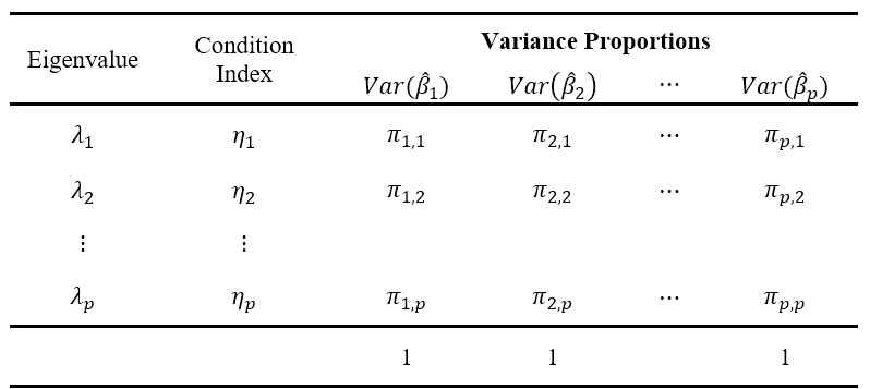
Variance Proportions
By the Spectral Decomposition, we can decompose the matrix form of the variance of the estimated coefficients as \[ Var(\hat{\boldsymbol{\beta}})=\sigma^2(\textbf{X}'\textbf{X})^{-1}= \sigma^2\textbf{T}\boldsymbol{\Lambda}^{-1}\textbf{T}' \] where
- \(\textbf{T}\) is a \(p \times p\) matrix composed of columns of eigenvectors \(\textbf{t}_k\) of \(\textbf{X}'\textbf{X}\) corresponding to \(k^{th}\) eigenvalue. \[ \begin{align} \textbf{T}&=\begin{bmatrix}\textbf{t}_1 & \textbf{t}_2 & \cdots & \textbf{t}_p\end{bmatrix}\\ &=\begin{bmatrix}t_{11} & t_{12} & \cdots & t_{1p} \\ t_{21} & t_{22} & \cdots & t_{2p} \\ \vdots & \vdots &\ddots&\vdots \\ t_{p1} & t_{p2} & \cdots & t_{pp}\end{bmatrix}\\ \end{align} \]
- \(\boldsymbol{\Lambda}\) is a diagonal matrix composed of eigenvalues of \(\textbf{X}'\textbf{X}\). \[ \boldsymbol{\Lambda}=\text{diag}(\lambda_1,\lambda_2,\cdots,\lambda_p) \]
Note that from here, \[ Var(\hat{\beta_j})=\sigma^2 \sum_{k=1}^p \frac{t^2_{jk}}{\lambda_k} \]
Definition 12.6 Variance Proportion of the \(j^{th}\) regressor with the \(i^{th}\) eigenvector is given by: \[ \pi_{j,i}=\frac{t_{ji}^2/\lambda_i}{\sum_{k=1}^p {t^2_{jk}}/{\lambda_k}} \]
Rationale
recall from the definition of multicollinearity: There exists \(c_1,c_2,...,c_p\) (not all zero) such that \[ c_1\textbf{x}_1+c_2\textbf{x}_2+\cdots+c_p\textbf{x}_p=\textbf{0} \quad (\text{or} \approx\textbf{0}) \]
If \(\lambda_j\) is close to 0, and \(\textbf{t}_j=\begin{bmatrix}t_{j1} & t_{j2} & \cdots & t_{jk}\end{bmatrix}'\) is the eigenvector associated with \(\lambda_j\), then \(\sum_{i=1}^k t_{ji}X_i\approx0\) gives the structure of dependency of the Xs that leads to the problem of multicollinearity.
a high proportion of any variance can be associated with a large singular value even when there is no perfect collinearity.
Rule:
The standard approach is to check a high condition index (usually >30) associated with a large proportion of the variance of two or more coefficients when diagnosing collinearity.
If two or more elements in the \(j^{th}\) condition index are relatively large and its associated condition index \(\eta_j\) is large too, it signals that near dependencies are influencing regression estimates.
That is, a multicollinearity problem occurs when a component associated with a high condition index contributes strongly (variance proportion greater than about 0.5) to the variance of two or more variables.
To summarize, collinearity is spotted by finding 2 or more variables that have large proportions of variance (0.50 or more) that correspond to large condition indices (>30).
To detect multicollinearity, we may ask the following questions:
Which regressors have coefficients with very inflated variance due to multicollinearity?
use the variance inflation factors
Is there an overall problem of multicollinearity or dependencies between the regressors?
use the condition number
How many dependency structures are there?
use the condition indices
Which are the variables involved in these dependencies?
use the variance proportions
Illustration of Multicollinearity Diagnostics in R
The ols_coll_diag() function from the olsrr package shows the different multicollinearity diagnostics in a single output: VIF, Condition Index, and Variance Proportions.
| Variables | Tolerance | VIF |
|---|---|---|
| age | 0.5672772 | 1.762807 |
| weight | 0.1188067 | 8.417035 |
| bsa | 0.1876612 | 5.328752 |
| dur | 0.8082053 | 1.237309 |
| pulse | 0.2265737 | 4.413575 |
| stress | 0.5450051 | 1.834845 |
| Eigenvalue | Condition Index | intercept | age | weight | bsa | dur | pulse | stress | |
|---|---|---|---|---|---|---|---|---|---|
| 1 | 6.6558 | 1.0000 | 0.0000 | 0.0000 | 0.0000 | 0.0000 | 0.0016 | 0.0000 | 0.0030 |
| 2 | 0.2679 | 4.9842 | 0.0002 | 0.0001 | 0.0000 | 0.0001 | 0.0000 | 0.0000 | 0.5512 |
| 3 | 0.0714 | 9.6536 | 0.0005 | 0.0004 | 0.0001 | 0.0003 | 0.9285 | 0.0002 | 0.0524 |
| 4 | 0.0027 | 50.0668 | 0.1027 | 0.0890 | 0.0052 | 0.1698 | 0.0007 | 0.0040 | 0.0254 |
| 5 | 0.0011 | 77.3965 | 0.3723 | 0.7775 | 0.0092 | 0.0113 | 0.0259 | 0.0050 | 0.0391 |
| 6 | 0.0009 | 83.7514 | 0.2900 | 0.0381 | 0.0061 | 0.0736 | 0.0432 | 0.4376 | 0.1433 |
| 7 | 0.0002 | 201.4958 | 0.2343 | 0.0949 | 0.9794 | 0.7450 | 0.0000 | 0.5532 | 0.1856 |
Interpretation:
The variances of the estimated coefficients of
weightandbsaare inflated due to multicollinearity (\(\text{VIF}>5)\). This tells us that the variance of the estimated coefficient ofweightis inflated by a factor of 8.42 becauseweightis highly correlated with at least one of the other predictors in the model.The condition number implies that there is an overall problem of multicollinearity.
We check the variance proportions corresponding to condition indices >30.
The 4th to 6th condition indices are greater than 50, but there are no triples of variables with variance proportions > 0.5
The variance proportions of
weight,bsa, andpulsecorresponding to \(\eta_7=201.4958\) show that > 0.50.This implies that there is a possible multicollinearity structure among these variables:
\[ c_1\textbf{weight} + c_2\textbf{bsa} + c_3\textbf{pulse} \approx \textbf{0} \]
Furthermore, the eigensystem can describe the structure of the (near) dependency as
\[t_{71}\textbf{intercept}+t_{72}\textbf{age}+t_{73}\textbf{weight}+t_{74}\textbf{bsa}+t_{75}\textbf{dur}+t_{76}\textbf{pulse}+t_{77}\textbf{stress}\approx\textbf{0}\]
where \(\textbf{t}_j=\begin{bmatrix}t_{j1} & t_{j2} & \cdots & t_{jp}\end{bmatrix}'\) is the eigenvector corresponding to \(j^{th}\) eigenvalue.
12.4 Remedial Measures
No single solution can eliminate multicollinearity completely. Certain approaches may be useful.
Deletion of unimportant or redundant variables
- If a variable is redundant, it should have never been included in the model in the first place.
- You may also use variable selection procedures
Example
Recall blood pressure dataset.
bp(blood pressure in mm Hg)age(in years)weight(in kg)bsa(body surface area in sqm)dur(duration of hypertension in years)pulse(basal pulse in beats per minute)stress(stress index)
| patient | bp | age | weight | bsa | dur | pulse | stress |
|---|---|---|---|---|---|---|---|
| 1 | 105 | 47 | 85.4 | 1.75 | 5.1 | 63 | 33 |
| 2 | 115 | 49 | 94.2 | 2.10 | 3.8 | 70 | 14 |
| 3 | 116 | 49 | 95.3 | 1.98 | 8.2 | 72 | 10 |
| 4 | 117 | 50 | 94.7 | 2.01 | 5.8 | 73 | 99 |
| 5 | 112 | 51 | 89.4 | 1.89 | 7.0 | 72 | 95 |
| 6 | 121 | 48 | 99.5 | 2.25 | 9.3 | 71 | 10 |
| 7 | 121 | 49 | 99.8 | 2.25 | 2.5 | 69 | 42 |
| 8 | 110 | 47 | 90.9 | 1.90 | 6.2 | 66 | 8 |
| 9 | 110 | 49 | 89.2 | 1.83 | 7.1 | 69 | 62 |
| 10 | 114 | 48 | 92.7 | 2.07 | 5.6 | 64 | 35 |
| 11 | 114 | 47 | 94.4 | 2.07 | 5.3 | 74 | 90 |
| 12 | 115 | 49 | 94.1 | 1.98 | 5.6 | 71 | 21 |
| 13 | 114 | 50 | 91.6 | 2.05 | 10.2 | 68 | 47 |
| 14 | 106 | 45 | 87.1 | 1.92 | 5.6 | 67 | 80 |
| 15 | 125 | 52 | 101.3 | 2.19 | 10.0 | 76 | 98 |
| 16 | 114 | 46 | 94.5 | 1.98 | 7.4 | 69 | 95 |
| 17 | 106 | 46 | 87.0 | 1.87 | 3.6 | 62 | 18 |
| 18 | 113 | 46 | 94.5 | 1.90 | 4.3 | 70 | 12 |
| 19 | 110 | 48 | 90.5 | 1.88 | 9.0 | 71 | 99 |
| 20 | 122 | 56 | 95.7 | 2.09 | 7.0 | 75 | 99 |
cor_matrix <- cor(bloodpressure[,2:8])
corrplot::corrplot(cor_matrix, method = "shade", addCoef.col = 'grey')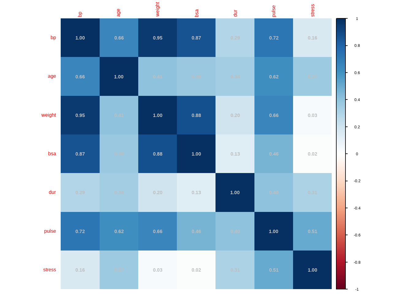
We first check the variance inflation factors for detecting multicollinearity:
full_bp <- lm(bp ~ age + weight + bsa + dur + pulse + stress,
data = bloodpressure)
car::vif(full_bp)## age weight bsa dur pulse stress
## 1.762807 8.417035 5.328751 1.237309 4.413575 1.834845We can either manually select unimportant variables based on literature, or use an automatic variable selection procedure. For this example, we use backward elimination based on sequential F-tests \(\alpha=0.05\).
## Backward Elimination Method
## ---------------------------
##
## Candidate Terms:
##
## 1. age
## 2. weight
## 3. bsa
## 4. dur
## 5. pulse
## 6. stress
##
##
## Step => 0
## Model => bp ~ age + weight + bsa + dur + pulse + stress
## R2 => 0.996
##
## Initiating stepwise selection...
##
## Step => 1
## Removed => dur
## Model => bp ~ age + weight + bsa + pulse + stress
## R2 => 0.99556
##
## Step => 2
## Removed => pulse
## Model => bp ~ age + weight + bsa + stress
## R2 => 0.99493
##
## Step => 3
## Removed => stress
## Model => bp ~ age + weight + bsa
## R2 => 0.99454
##
##
## No more variables to be removed.
##
## Variables Removed:
##
## => dur
## => pulse
## => stressAfter a backward elimination algorithm the independent variables selected for predicting blood pressure are age, weight, and body surface area.
##
## Call:
## lm(formula = paste(response, "~", paste(c(include, cterms), collapse = " + ")),
## data = l)
##
## Residuals:
## Min 1Q Median 3Q Max
## -0.75810 -0.24872 0.01925 0.29509 0.63030
##
## Coefficients:
## Estimate Std. Error t value Pr(>|t|)
## (Intercept) -13.66725 2.64664 -5.164 9.42e-05 ***
## age 0.70162 0.04396 15.961 3.00e-11 ***
## weight 0.90582 0.04899 18.490 3.20e-12 ***
## bsa 4.62739 1.52107 3.042 0.00776 **
## ---
## Signif. codes: 0 '***' 0.001 '**' 0.01 '*' 0.05 '.' 0.1 ' ' 1
##
## Residual standard error: 0.437 on 16 degrees of freedom
## Multiple R-squared: 0.9945, Adjusted R-squared: 0.9935
## F-statistic: 971.9 on 3 and 16 DF, p-value: < 2.2e-16Now, checking for multicollinearity:
## age weight bsa
## 1.201901 4.403645 4.286943This model may help individuals estimate their own blood pressures using only their age, weight, and body surface area.
Centering of observations
Centering a predictor is subtracting the mean of the predictor values in the data set from each predictor value. \(X_i \rightarrow (X_i-\bar{X})\)
This is especially effective if complex functions of X’s (e.g. \(f(X)=X^2\)) are present in the design matrix. After centering, the non-linear relationship of \(X\) and \(f(X)\) will be more apparent, and the collinearity issue will be solved.
An example of including both \(X\) and a complex function of \(X\) in the model:
- suppose \(Y\) and \(X\) have a quadratic relationship, and can be characterized using a polynomial model:
\[ y_i = \beta_0 +\beta_1X_{i} + \beta_2X_{i}^2+\varepsilon_i \]
We can use OLS to estimate \(\beta_1\) and \(\beta_2\), but for some range of values of \(X\), \(X\) and \(X^2\) may look like linearly related (near linearity). This is an example of Structural Multicollinearity.
as a solution, center the Xs, and fit the following line instead:
\[ y_i = \beta_0^* +\beta_1^*(X_{i}-\bar{X}) + \beta_2^*(X_{i}-\bar{X})^2+\varepsilon_i \]
- Multicollinearity will be solved in such a way that the nonlinearity of \(X\) and \(X^2\) will be more defined and apparent in the datapoints.
Example
According to researchers, amount of immunoglobin in the blood (igg) and the maximal oxygen uptake (oxygen) of an individual can be modeled using a quadratic (polynomial) equation.
\[ igg_i=\beta_0+\beta_1oxygen + \beta_{2} (oxygen)^2 + \varepsilon_i \]
Notice that both oxygen and some complex function of oxygen are both regressors in the model.
| igg | oxygen |
|---|---|
| 881 | 34.6 |
| 1290 | 45.0 |
| 2147 | 62.3 |
| 1909 | 58.9 |
| 1282 | 42.5 |
| 1530 | 44.3 |
| 2067 | 67.9 |
| 1982 | 58.5 |
| 1019 | 35.6 |
| 1651 | 49.6 |
| 752 | 33.0 |
| 1687 | 52.0 |
| 1782 | 61.4 |
| 1529 | 50.2 |
| 969 | 34.1 |
| 1660 | 52.5 |
| 2121 | 69.9 |
| 1382 | 38.8 |
| 1714 | 50.6 |
| 1959 | 69.4 |
| 1158 | 37.4 |
| 965 | 35.1 |
| 1456 | 43.0 |
| 1273 | 44.1 |
| 1418 | 49.8 |
| 1743 | 54.4 |
| 1997 | 68.5 |
| 2177 | 69.5 |
| 1965 | 63.0 |
| 1264 | 43.2 |
The goal is to estimate the parameters \(\beta_0\), \(\beta_1\), and \(\beta_{2}\)
Fitting the line \(igg_i=\beta_0+\beta_1oxygen + \beta_{2} (oxygen)^2 + \varepsilon_i\) on the data, using OLS, we have:
immunity$oxygen_sq <- immunity$oxygen^2
immunity_model <- lm(igg ~ oxygen + oxygen_sq, data = immunity)
immunity_model##
## Call:
## lm(formula = igg ~ oxygen + oxygen_sq, data = immunity)
##
## Coefficients:
## (Intercept) oxygen oxygen_sq
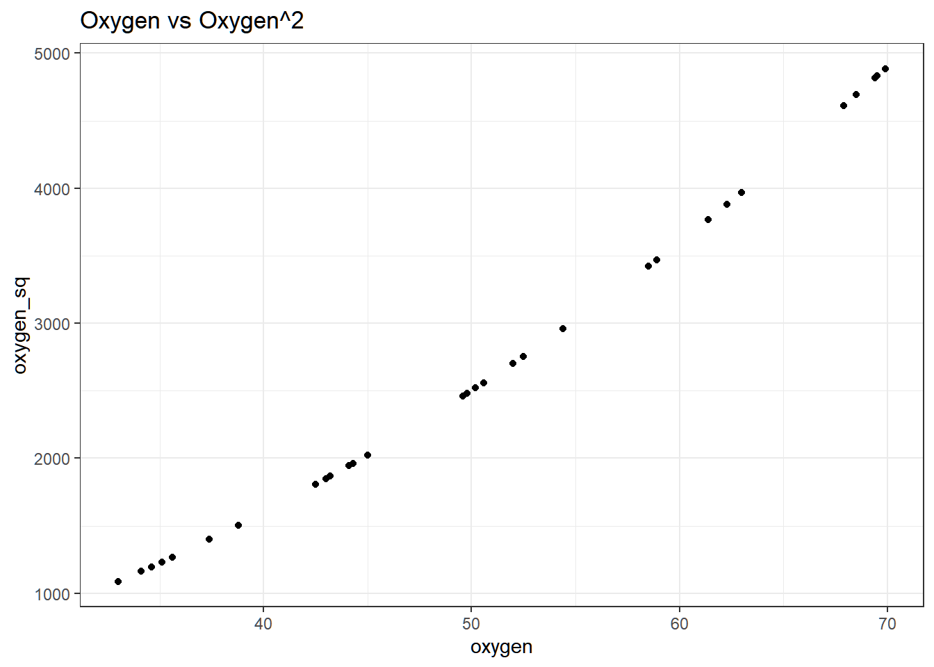
## -1464.4042 88.3071 -0.5362Plotting the fitted line \(\widehat{igg}_i=\hat{\beta_1} + \hat{\beta_1}oxygen_i + \hat{\beta}_{2}oxygen^2_i\), we have:
The line is good in such a way that it passes through the center of the points. However, near multicollinearity exists between \(oxygen\) and \(oxygen^2\), even if the relationship is nonlinear. To visualize:
Variance of \(\hat{\beta}_1\) and \(\hat{\beta}_{2}\) are both inflated, indicated by the \(\text{VIF}\).
## oxygen oxygen_sq
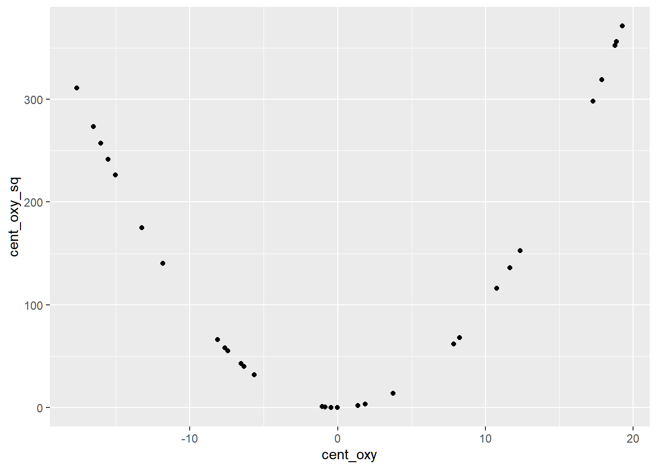
## 99.94261 99.94261As a solution, we center the observed values of \(oxygen\rightarrow\) cent_oxy = oxygen - mean(oxygen)
Centering \(X\), we can formulate the model as:
\[ y_i = \beta_0 +\beta_1^*(X_{i}-\bar{X}) + \beta_{2}^*(X_{i}-\bar{X})^2+\varepsilon_i \]
immunity <- immunity %>%
mutate(
cent_oxy = oxygen - mean(oxygen),
cent_oxy_sq = (oxygen - mean(oxygen))^2
)The centered variables now have more defined nonlinear relationship.
We expect that multicollinearity between the two variables will be solved.
##
## Call:
## lm(formula = igg ~ cent_oxy + cent_oxy_sq, data = immunity)
##
## Coefficients:
## (Intercept) cent_oxy cent_oxy_sq
## 1632.1962 33.9995 -0.5362The fitted line can be expressed as
\[ \hat{y}_i = 1632.1962 + 33.9995(X_i - mean(X)) - 0.5362 (X_i - mean(X))^2 \]
Plotting the fitted line on the data:
# original fitted line
fitted_immunity <- function(x){
# defining estimated parameters
beta_0 = coef(immunity_model)["(Intercept)"]
beta_1 = coef(immunity_model)["oxygen"]
beta_11 = coef(immunity_model)["oxygen_sq"]
# expressing the equation
y = beta_0 + beta_1*x +beta_11*x^2
return(y)
}
# new equation after centering
fitted_cnter <- function(x){
imm_model_cntr$coefficients[1] +
imm_model_cntr$coefficients[2]*(x-mean(immunity$oxygen)) + imm_model_cntr$coefficients[3]*(x-mean(immunity$oxygen))^2
}ggplot(immunity)+
geom_point(aes(x = oxygen, y = igg))+
geom_function(fun = fitted_immunity,
aes(color = "fun1"),
lwd = 1,
linetype = 1) +
geom_function(fun = fitted_cnter,
aes(color = "fun2"),
lwd = 1,
linetype = 1)+
scale_color_manual(values = c(fun1 = "red", fun2 = "green"),
labels = c(expression(hat(y)==-1464.40 + 88.30*x -0.54*x^2),
expression(hat(y)== 1632.19 + 33.99*(x-bar(x)) - 0.54*(x-bar(x))^2)))+
theme_bw()+
theme(legend.title=element_blank(),
legend.position=c(.3,.9)
)## Warning in geom_function(fun = fitted_immunity, aes(color = "fun1"), lwd = 1, : All aesthetics have length 1, but the data has 30 rows.
## ℹ Please consider using `annotate()` or provide this layer with data containing a single row.## Warning in geom_function(fun = fitted_cnter, aes(color = "fun2"), lwd = 1, : All aesthetics have length 1, but the data has 30 rows.
## ℹ Please consider using `annotate()` or provide this layer with data containing a single row.
The VIF of the parameters are now lower.
## cent_oxy cent_oxy_sq
## 1.050628 1.050628Shrinkage Estimation (Ridge Regression)
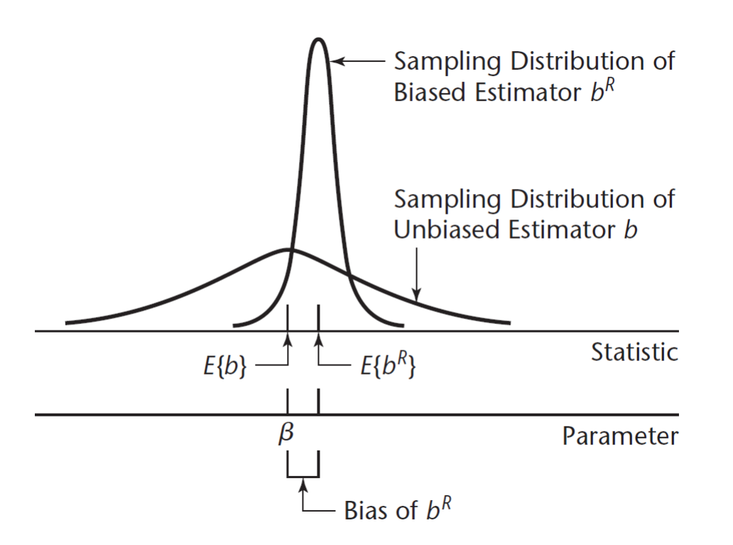
Instead of using the OLS estimator, we use another estimator that has less inflated variance, but compromises the unbiasedness.
In Ridge regression, the Normal Equations is given by \(\left(\textbf{X}'\textbf{X}+k \textbf{I}\right) \hat{\boldsymbol{\beta}}_R = \textbf{X}'\textbf{Y}\), where \(k\geq 0\) is called the biasing parameter.
The ridge estimator is \(\hat{\boldsymbol{\beta}}_R = \left(\textbf{X}'\textbf{X}+k \textbf{I}\right)^{-1} \textbf{X}'\textbf{Y}\)
\(k\) is usually chosen to be a number between 0 and 1.
If \(k=0\) then the ridge estimator reduces to OLS estimator.
If \(k\) is very large, the coefficients will become 0.
\[ \lim_{k\rightarrow \infty} (\hat{\boldsymbol\beta}_R)=\boldsymbol{0} \]
Properties of Ridge Estimator
The ridge estimator is a linear transformation of the OLS estimator. Hence, it is also a linear estimator of \(\boldsymbol{\beta}\).
Expected value
\[ E(\hat{\boldsymbol{\beta}}_R)=(\textbf{X}'\textbf{X}+k \textbf{I})^{-1} \textbf{X}'\textbf{X}\boldsymbol{\beta} \]
This implies that \(\hat{\boldsymbol{\beta}}_R\) is a biased estimator.
Bias
\[ Bias(\hat{\boldsymbol{\beta}}_R) = E(\hat{\boldsymbol{\beta}}_R)-\boldsymbol{\beta}=((\textbf{X}'\textbf{X}+k \textbf{I})^{-1} \textbf{X}'\textbf{X}-\textbf{I})\boldsymbol{\beta} \]
Variance
\[ Var(\hat{\boldsymbol{\beta}}_R)=\sigma^2(\textbf{X}'\textbf{X}+k \textbf{I})^{-1} (\textbf{X}'\textbf{X})(\textbf{X}'\textbf{X}+k \textbf{I})^{-1} \]
Bias-Variance decomposition of MSE
The following measures provide scalar measures of overall estimation biasedness and uncertainty:
Sum of squares of bias of the ridge estimators:
\[ \begin{align} \sum_{j=1}^pBias(\hat{\beta}_{R,j})^2 &=tr(Bias(\hat{\boldsymbol{\beta}}_R)^2)\\ &=Bias(\hat{\boldsymbol{\beta}}_R)^TBias(\hat{\boldsymbol{\beta}}_R)\\ &=k^2\boldsymbol{\beta}'(\textbf{X}'\textbf{X}+k \textbf{I})^{-1}\boldsymbol{\beta} \end{align} \]
Total variance of the ridge estimators of each coefficent.
\[ \sum_{j=1}^pVar(\hat{\beta}_{R,j})=tr\left(Var(\hat{\boldsymbol{\beta}}_R)\right)=\sigma^2\sum_{j=1}^p\frac{\lambda_j}{(\lambda_j+k)^2} \]
where \(\lambda_j\) is the \(j^{th}\) eigenvalue of the covariance matrix of \(\hat{\boldsymbol{\beta}}_R\)
The mean square error of \(\hat{\boldsymbol{\beta}}_R\) in estimating \(\boldsymbol\beta\) can be decomposed as:
\[ \begin{align} MSE_{\boldsymbol\beta}(\hat{\boldsymbol\beta}_R) &= E\left((\hat{\boldsymbol\beta}_R-\boldsymbol\beta)^T(\hat{\boldsymbol\beta}_R-\boldsymbol\beta)\right)\\ &= tr\left(Bias(\hat{\boldsymbol{\beta}}_R)^2\right) + tr\left(Var(\hat{\boldsymbol{\beta}}_R)\right)\\ &= \underbrace{k^2\boldsymbol{\beta}'(\textbf{X}'\textbf{X}+k \textbf{I})^{-1}\boldsymbol{\beta}}_{\text{increases with }k} + \underbrace{\sigma^2\sum_{j=1}^p\frac{\lambda_j}{(\lambda_j+k)^2}}_{\text{decreases with }k} \end{align} \]
Bias-Variance tradeoff
From the formulas in the bias-variance decomposition, as the biasing parameter \(k\) increases, the total variance of ridge estimator \(\hat{\boldsymbol{\beta}}_R\) “shrinks” (more reliable) but the Bias increases (less accurate).
Ridge regression will not necessarily give the best fit in terms of unbiasedness, but will surely give more stable (reliable) estimates.
Determination of \(k\)
We want a value of \(k\) that makes estimates for the coefficients more stable, but does not compromise the unbiasedness that much.
Ridge Trace
Plot the estimates of the parameters for some values of \(k\) between 0 and 1. Choose smallest value of \(k\) where the trace starts to stabilize.
VIF Trace
Plot the VIF of the parameters for some values of \(k\) between 0 and 1. Choose smallest value of \(k\) where all \(VIF\) are less than your set threshold (less than 5)
Example in R
We use the bloodpressure data again. Recall the VIF of the parameters:
##      age   weight      bsa      dur    pulse   stress
## 1.762807 8.417035 5.328751 1.237309 4.413575 1.834845The lmridge package can help perform ridge regression. We try for different values of the biasing parameter \(k\).
library(lmridge)
bp_ridge_trace <- lmridge(bp~age+weight+bsa+dur+pulse+stress,
                    data=bloodpressure,
                    K = seq(0,1,0.005))
In selecting the value of the biasing parameter \(k\), we check at what value of \(k\) will the estimates become to stabilize.

We can also look at the changes of \(VIF\) as \(k\) increases. We want the lowest value of \(k\) where the \(VIF\) are all less than 5.
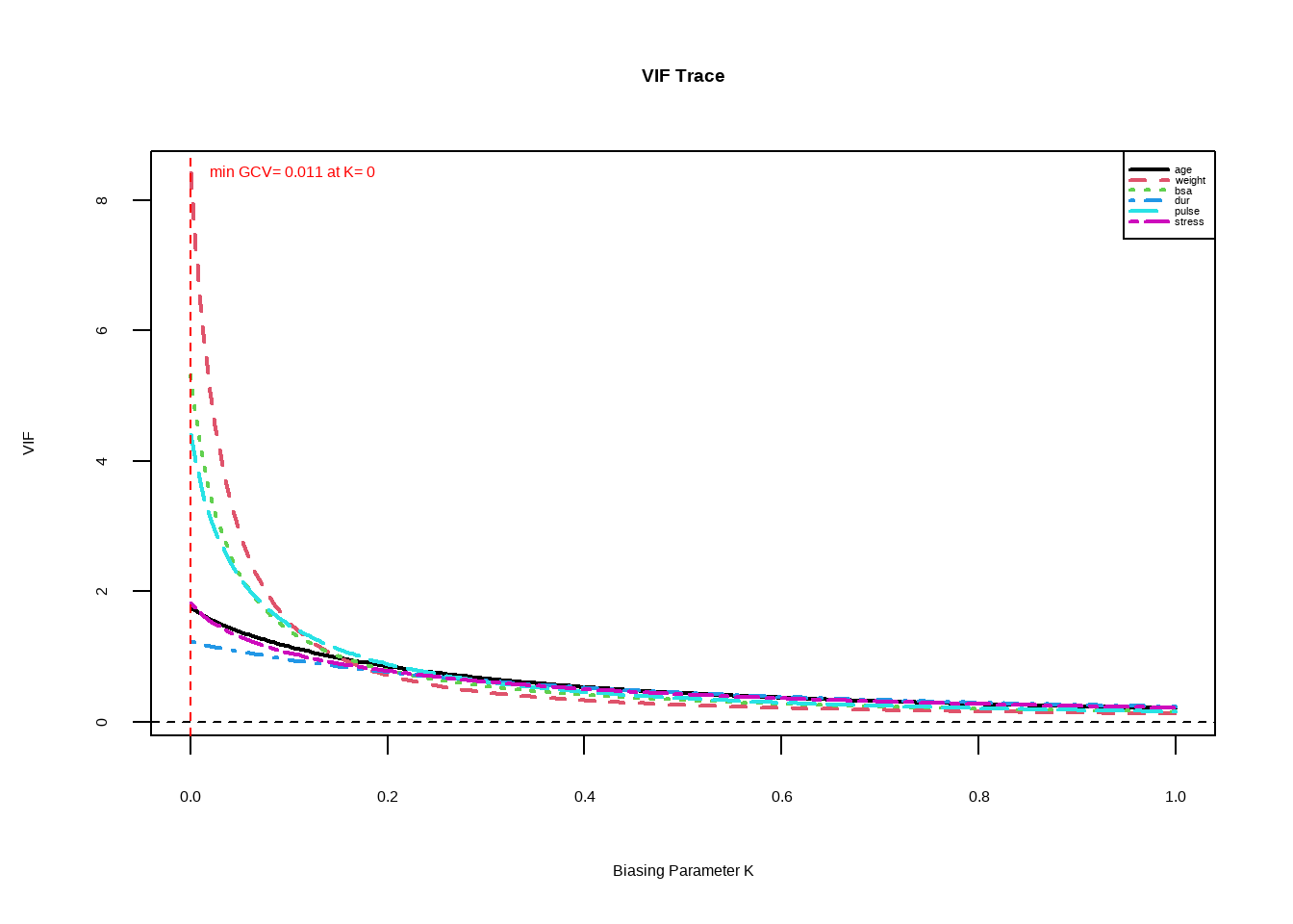
We select \(k=0.1\)
bp_ridge <- lmridge(bp~age+weight+bsa+dur+pulse+stress,
                    data=bloodpressure,
                    K = 0.1)
summary(bp_ridge)
##
## Call:
## lmridge.default(formula = bp ~ age + weight + bsa + dur + pulse +
## stress, data = bloodpressure, K = 0.1)
##
##
## Coefficients: for Ridge parameter K= 0.1
## Estimate Estimate (Sc) StdErr (Sc) t-value (Sc) Pr(>|t|)
## Intercept -3.1368 -1458.8787 116.2184 -12.5529 <2e-16 ***
## age 0.5855 6.3815 0.7711 8.2755 <2e-16 ***
## weight 0.6390 11.9620 0.8867 13.4900 <2e-16 ***
## bsa 9.9908 5.9437 0.8488 7.0028 <2e-16 ***
## dur 0.0773 0.7231 0.7010 1.0314 0.3195
## pulse 0.1268 2.1024 0.8752 2.4021 0.0305 *
## stress -0.0016 -0.2560 0.7387 -0.3466 0.7340
## ---
## Signif. codes: 0 '***' 0.001 '**' 0.01 '*' 0.05 '.' 0.1 ' ' 1
##
## Ridge Summary
## R2 adj-R2 DF ridge F AIC BIC
## 0.90670 0.87340 4.76418 181.43035 -10.31040 54.34809
## Ridge minimum MSE= 71.22473 at K= 0.1
## P-value for F-test ( 4.76418 , 14.47388 ) = 1.885411e-12
## -------------------------------------------------------------------Now, the VIF of the parameters are now lower.
##          age  weight     bsa     dur   pulse  stress
## k=0.1 1.1604 1.53437 1.40577 0.95903 1.49481 1.06477
What is the advantage of Ridge Regression over Least Squares?
Well, first, it is a remedial measure for multicollinearity.
Ridge regression’s advantage over least squares is rooted in the bias-variance trade-off. As the biasing parameter \(k\) increases, the flexibility of the ridge regression fit decreases,leading to decreased variance but increased bias.
Imposing Constraints
Suppose your model is \[ Y=\beta_0+\beta_1X_1+\beta_2X_2+\beta_3X_3+\varepsilon \] The eigensystem analysis suggests that there are regressors that are linearly related, for example, \(2X_1+X_2=0\).
To fit the model , we can combine \(X_1\) and \(X_2\) by imposing constraint \(\beta_1=2\beta_2\).
Inserting the restriction, rewriting the original regression model, we will get
\[ \begin{align} Y&=\beta_0+2\beta_2X_1+\beta_2X_2+\beta_3X_3+\varepsilon\\ &=\beta_0+\beta_2(2X_1+X_2)+\beta_3X_3+\varepsilon\\ &=\beta_0+\beta_2Z+\beta_3X_3+\varepsilon \end{align} \] This will have an effect of regressing on the new variable \(Z\) rather than each of \(X_1\) and \(X_2\).
Transform or Combine Multicollinear Variables
You can perform dimension reduction procedures while still using all available variables. Combination of multicollinear variables will help.
For example, instead of including both \(GDP\) and \(population\) in the model (which may be correlated), include \(\frac{GDP}{population}=\text{GDP per capita}\).
Another method is the Principal Component Regression. The idea is that it combines related variables as “Principal Components”, which will be used as the regressors in the model.
Example of Principal Component Regression
In the following example, we model the price of
bangusbased on different factors:prices of different goods (
gg,tilapia,pork,chicken)economic indicators
cpi: Consumer Price Indexcpifbt: Consumer Price Index of Food, Beverage, and Tobaco
a climate variable
soi: Southern Oscillation Index
…1 cpi cpifbt bangus gg tilapia pork chicken soi 1 46.3 45.1 12.92 8.17 12.64 16.90 14.58 -2.6 2 47.6 46.4 12.40 8.84 11.98 16.76 14.50 -3.2 3 48.0 46.8 12.39 9.16 5.10 17.15 14.83 -4.0 4 48.3 47.2 12.12 9.41 7.20 17.24 14.65 -3.3 5 48.5 47.3 12.05 8.53 6.53 17.61 14.36 -3.6 6 48.9 47.7 12.09 8.43 9.43 16.63 14.15 -5.1 7 49.0 47.8 12.67 8.56 9.91 16.40 15.09 -4.6 8 46.1 44.4 12.80 9.90 10.14 18.87 15.43 -6.9 9 46.3 44.6 12.51 9.81 10.95 19.07 15.04 -7.6 10 46.5 44.7 12.76 9.27 11.25 18.99 15.07 -5.6 11 46.8 45.1 13.16 8.89 11.76 19.02 14.97 -2.2 12 47.2 45.7 12.42 8.32 10.78 19.08 14.99 0.7 13 47.9 46.5 11.78 8.67 11.33 19.06 14.89 -0.5 14 49.0 47.5 11.22 8.52 10.60 18.95 15.21 -1.3 15 49.9 48.4 11.63 9.34 11.03 19.03 14.70 -0.3 16 50.2 48.6 12.24 9.24 10.43 19.04 16.10 1.7 17 50.6 49.1 13.07 10.38 10.63 19.28 15.98 0.4 18 53.3 51.9 14.37 11.61 11.74 20.89 17.62 -0.3 19 57.5 56.6 13.77 14.49 14.30 22.61 19.12 -0.2 20 60.1 59.3 18.78 14.93 15.20 23.35 19.91 0.2 21 62.3 61.5 19.92 15.98 16.19 27.63 20.82 0.9 22 63.6 63.1 20.63 15.58 15.75 29.34 20.34 -1.5 23 64.7 64.2 21.25 15.69 16.71 30.63 21.44 0.3 24 65.6 65.2 20.51 14.50 16.07 32.46 22.35 -0.1 25 69.4 69.2 20.69 15.22 16.81 34.95 23.64 -1.3 26 75.8 74.9 20.40 16.71 19.09 36.36 25.15 0.1 27 77.8 76.9 21.47 18.64 18.47 35.97 24.99 0.1 28 79.9 79.6 22.07 19.38 18.50 35.68 25.85 0.2 29 81.3 81.3 22.11 19.77 19.03 34.50 25.30 -1.0 30 84.3 84.5 24.35 22.12 20.56 35.84 26.40 0.4 31 85.6 85.9 25.78 23.02 21.86 35.83 26.06 -0.7 32 87.9 87.9 27.98 22.94 23.05 37.30 28.17 -0.7 33 88.8 89.3 27.07 20.71 21.40 37.42 28.33 1.7 34 89.2 89.3 26.09 18.80 20.68 37.21 26.67 0.3 35 88.6 88.6 26.39 17.97 20.50 37.93 27.85 1.7 36 88.7 88.5 24.90 17.78 19.98 36.33 27.15 0.3 37 88.9 88.6 25.12 20.42 20.75 38.99 27.34 -1.5 38 90.4 89.8 25.93 20.32 21.25 37.17 27.90 -0.4 39 90.6 90.1 27.20 20.68 21.19 36.80 26.60 1.1 40 90.4 89.5 26.29 21.28 21.34 36.53 27.54 -0.1 41 89.9 88.6 26.70 22.50 22.22 37.75 27.36 -1.2 42 90.1 88.8 27.58 21.51 22.54 36.82 27.62 -0.5 43 90.3 89.0 29.70 22.67 28.34 37.22 27.88 0.2 44 90.5 89.9 35.09 24.99 26.44 40.54 31.78 1.5 45 91.3 90.9 34.73 22.51 25.57 42.03 31.11 -2.7 46 91.5 90.9 30.97 20.73 23.42 40.57 30.25 -0.1 47 89.6 88.4 30.06 17.44 21.68 41.41 28.44 0.1 48 88.9 87.3 27.65 18.48 21.42 41.86 27.00 -0.9 49 88.1 86.1 27.45 18.07 21.92 41.82 28.73 1.1 50 87.9 85.8 27.36 19.45 21.77 40.25 28.28 0.2 51 87.8 85.7 27.70 21.09 22.01 40.48 28.06 -1.6 52 87.9 85.7 27.00 19.91 20.88 40.22 27.88 -1.0 53 88.2 86.2 26.30 19.34 19.73 41.64 27.87 0.9 54 89.0 87.4 28.58 21.99 20.82 41.74 28.05 -2.5 55 88.7 86.8 30.29 23.54 24.01 42.90 29.61 -3.0 56 89.3 87.9 33.00 24.27 25.33 41.32 32.49 -1.5 57 89.7 88.4 32.97 22.64 24.69 41.75 31.32 -3.1 58 89.7 88.3 31.33 19.44 22.86 42.09 30.94 -3.3 59 89.7 88.0 31.12 17.32 22.95 42.39 31.79 -3.0 60 90.5 89.3 29.82 16.64 22.85 43.23 32.36 -2.8 61 91.6 90.7 29.47 17.98 22.60 43.24 33.14 -2.8 62 92.7 92.1 28.06 19.12 22.04 44.05 34.24 -2.8 63 93.1 92.5 27.59 19.06 22.63 44.37 35.66 -2.5 64 93.3 92.8 27.55 20.12 21.80 44.29 36.14 -1.9 65 93.3 92.5 27.65 19.53 22.33 44.69 35.91 -1.1 66 93.8 93.1 28.64 20.87 25.27 45.34 35.05 -0.2 67 94.9 94.7 30.62 23.75 26.69 44.30 35.74 -1.2 68 96.7 96.6 31.19 22.04 25.37 39.54 36.22 -0.3 69 97.4 97.0 32.50 21.35 26.24 39.75 36.31 -1.4 70 98.2 97.7 32.05 21.71 26.13 39.73 36.46 0.1 71 98.4 98.1 37.03 21.23 27.54 41.46 35.78 -0.1 72 98.8 98.6 33.50 20.14 25.56 40.90 36.04 1.3 73 99.7 99.5 32.96 21.19 25.58 40.30 37.34 -0.4 74 100.4 100.3 31.19 22.59 23.90 40.86 37.55 1.7 75 100.9 100.8 30.84 22.14 23.75 41.41 38.62 2.2 76 101.2 100.9 30.40 21.72 23.78 42.40 37.27 3.4 77 101.4 101.2 31.30 22.27 26.09 41.83 37.39 2.2 78 102.9 103.7 33.40 24.85 27.46 42.81 38.70 3.0 79 104.0 105.5 38.73 28.88 30.15 43.74 39.83 2.1 80 106.3 108.2 48.59 30.12 34.14 44.93 42.16 2.7 81 107.0 108.6 46.52 28.91 34.31 45.01 41.06 1.8 82 107.0 108.2 45.98 26.43 33.46 45.87 41.86 1.0 83 108.0 109.3 44.27 23.78 32.77 46.96 40.75 2.6 84 109.1 110.9 43.41 24.52 32.30 49.34 40.94 1.9 85 111.1 112.3 43.64 24.46 32.92 50.35 41.02 0.8 86 112.4 113.8 43.13 25.54 34.94 51.28 40.02 1.4 87 114.9 117.3 43.91 27.65 36.24 51.39 40.88 -1.3 88 115.9 118.2 43.93 28.84 34.99 51.50 39.36 0.9 89 116.8 119.3 43.95 27.09 36.70 51.90 40.02 1.0 90 117.9 120.3 45.53 29.42 38.34 52.55 42.72 -0.6 91 120.1 122.1 48.77 31.15 40.06 52.44 45.21 -1.2 92 122.2 123.2 45.47 28.35 34.51 52.27 44.42 -0.4 93 122.4 123.0 46.16 24.86 35.19 57.63 40.16 -3.9 94 123.0 123.1 46.35 27.05 32.21 53.18 43.41 -1.9 95 124.0 123.8 46.87 25.96 31.51 53.16 45.00 -0.1 96 124.8 124.9 46.80 22.84 32.51 53.14 44.14 1.8 97 126.1 125.9 46.44 23.30 32.81 53.23 43.35 -0.1 98 128.1 127.7 45.57 24.54 33.98 53.18 43.78 0.8 99 128.9 128.4 45.44 25.80 34.52 52.86 44.83 -1.0 100 130.2 129.8 45.44 25.53 33.75 53.40 45.25 -1.3 101 132.7 131.6 46.05 26.02 33.74 54.07 46.09 0.1 102 135.2 133.5 47.51 29.96 37.23 53.92 46.28 -1.1 103 139.5 136.6 49.70 32.92 38.65 56.48 48.67 -0.7 104 143.7 140.6 51.93 30.96 37.95 57.53 50.33 1.0 105 146.8 143.0 52.46 27.83 37.18 57.98 48.86 -0.1 106 148.1 143.8 53.21 28.30 38.91 58.49 48.62 -2.2 107 149.1 144.5 53.67 26.59 38.82 59.80 48.59 -1.7 108 149.9 145.2 52.91 25.91 38.35 61.51 49.16 -2.4 109 151.5 146.0 52.57 26.41 39.53 62.89 49.35 -0.9 110 152.9 147.5 52.86 27.90 40.62 62.86 47.75 -0.2 111 154.6 149.9 53.82 30.00 41.45 63.85 51.52 -1.4 112 156.4 151.5 54.63 31.91 42.50 65.01 55.82 -2.9 113 156.5 150.9 53.70 29.41 41.25 66.00 54.80 -2.4 114 157.1 151.5 54.87 30.33 41.56 67.01 54.04 -1.4 115 157.8 152.2 55.41 30.62 42.29 68.80 51.07 -3.7 116 159.2 153.0 62.68 35.03 50.42 70.21 55.49 -5.6 117 159.8 152.9 62.59 33.31 48.30 70.73 52.31 -2.3 118 161.1 152.9 62.45 30.43 49.07 69.42 52.54 -4.8 119 162.0 153.4 63.04 29.11 48.98 70.06 53.23 -2.3 120 163.7 154.9 62.28 28.56 48.63 70.66 52.53 0.1 121 165.4 156.5 59.46 28.57 48.99 71.65 53.72 -1.9 122 167.0 157.9 56.75 27.49 48.97 72.20 56.42 -1.3 123 168.3 159.4 54.21 29.88 49.55 72.15 61.08 0.0 124 169.6 161.4 54.19 32.18 49.00 72.54 58.47 0.0 125 170.0 161.5 55.30 32.45 45.95 72.65 54.87 -3.2 126 170.5 161.8 56.12 35.60 50.67 71.45 54.15 -1.4 127 170.7 161.7 57.19 35.49 51.90 72.09 57.64 -1.4 128 172.3 162.3 58.98 35.58 51.81 71.12 54.97 -2.0 129 172.9 162.4 58.22 34.20 53.30 71.28 54.05 -2.1 130 173.6 162.3 59.94 24.40 52.20 71.20 51.24 -1.8 131 174.0 162.6 59.40 30.65 51.70 70.33 52.82 -2.6 132 174.6 162.9 62.05 30.71 45.99 69.42 53.88 -1.0 133 176.4 163.8 59.72 30.66 49.62 71.15 52.57 -2.2 134 178.9 166.8 59.34 32.59 50.71 70.19 52.93 -1.8 135 180.1 168.0 55.45 33.95 50.34 70.45 53.53 -2.4 136 182.4 171.2 56.28 32.61 49.98 70.32 54.62 -1.3 137 183.7 172.9 57.87 34.68 50.72 67.97 54.38 -2.5 138 184.1 173.1 59.24 35.87 51.13 68.13 55.57 -0.3 139 185.0 174.1 61.66 39.48 53.49 69.93 60.26 0.1 140 188.0 177.0 66.70 42.99 55.44 70.34 54.53 -0.5 141 191.0 177.4 68.05 42.67 58.06 72.15 55.97 -0.1 142 190.5 176.5 69.19 43.37 57.79 73.28 55.43 -2.2 143 191.0 176.7 70.70 37.41 56.61 74.72 54.35 -2.9 144 192.2 178.2 70.15 37.81 56.63 77.21 57.48 -1.7 145 193.7 179.3 66.71 37.06 57.11 79.07 57.32 -1.5 146 195.3 180.7 67.48 41.43 55.52 80.49 57.35 -2.9 147 197.8 184.4 66.49 40.96 55.44 80.82 58.14 -3.0 148 198.0 184.8 65.17 39.44 55.45 80.76 58.80 -3.0 149 198.0 184.5 64.33 40.14 53.51 80.49 52.65 -2.6 150 197.8 184.0 66.53 42.30 55.77 80.78 57.27 -1.2 151 198.3 184.4 70.34 41.78 57.11 80.78 60.26 -2.6 152 199.6 186.2 78.26 43.24 59.53 81.44 59.60 -1.0 153 200.4 186.3 80.42 40.86 61.49 81.05 57.07 -0.8 154 201.2 186.3 79.03 38.26 59.45 81.75 57.35 0.4 155 202.8 187.4 78.73 38.49 59.48 81.89 57.07 -1.8 156 205.2 190.2 76.12 38.26 57.96 82.11 56.31 -1.2 157 207.7 192.7 71.26 36.64 56.63 82.52 58.89 -0.4 158 209.8 195.4 69.97 38.10 56.04 81.66 59.16 0.6 159 213.8 201.8 68.02 39.20 55.19 81.00 61.84 -0.1 160 220.4 212.4 66.37 40.90 54.65 81.04 60.99 0.5 161 219.7 210.9 65.14 39.34 52.29 82.40 60.09 -0.5 162 219.7 212.2 63.64 40.88 53.97 79.59 59.61 -0.1 163 220.1 212.6 68.78 42.02 56.81 81.91 59.39 -1.3 164 221.9 213.9 73.16 47.93 59.20 82.63 58.46 1.7 165 224.1 216.1 77.48 47.14 58.14 82.79 56.52 -0.2 166 224.9 216.2 81.45 43.15 58.04 83.35 60.17 1.2 167 225.8 216.6 81.65 41.01 58.97 88.49 61.62 1.1 168 226.5 217.4 101.00 40.89 57.06 88.02 60.90 0.2 169 228.1 217.8 74.08 40.61 58.22 88.85 62.80 1.6 170 228.4 217.7 73.62 41.70 58.72 89.39 57.01 1.0 171 230.7 220.9 74.61 43.42 57.55 91.37 56.88 0.7 172 230.3 219.5 73.52 42.45 56.83 88.38 56.50 1.0 173 230.1 218.4 71.94 42.69 55.76 89.74 56.71 0.7 174 229.7 216.5 74.12 44.38 57.19 89.15 53.60 -0.3 175 231.5 217.9 75.70 44.64 58.44 90.05 56.31 1.3 176 233.0 218.5 78.08 44.12 57.95 89.85 56.66 0.8 177 234.0 218.5 81.30 45.69 59.49 89.95 56.67 2.6 178 235.8 220.4 82.74 49.34 60.33 89.45 56.31 -1.9 179 236.1 220.5 81.17 45.91 60.15 90.36 57.21 -1.4 180 236.0 220.1 78.83 44.07 60.10 90.70 58.61 -3.0 181 239.0 221.4 76.09 44.41 60.17 92.52 56.47 -3.2 182 239.3 220.9 72.80 44.13 58.60 93.25 57.41 -1.7 183 240.9 222.6 71.13 45.47 58.26 93.73 58.15 -3.4 184 242.2 223.8 69.47 44.48 56.68 93.09 56.52 -2.6 185 243.0 223.7 68.85 44.43 56.22 93.09 56.19 -3.1 186 244.4 224.3 68.83 45.49 56.77 93.26 57.28 -2.3 187 245.4 224.7 70.29 42.56 58.72 93.11 57.86 -2.1 We expect that some of the possible independent variables are correlated with each other.
cor_bangus <- dplyr::select(bangus,"cpi", "cpifbt", "gg":"soi") |> cor()
corrplot::corrplot(cor_bangus, method = "square", addCoef.col = 'grey')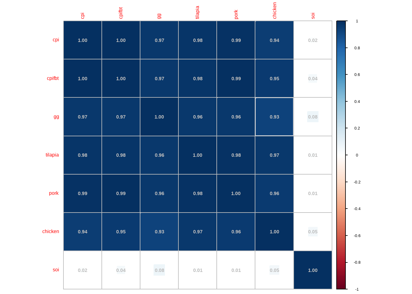
From the correlation plot, the Consumer Price Index and the prices of different goods are highly (almost perfect) correlated. Afterall, the CPI is a function of prices of different goods.
full_bangus <- lm(bangus~ cpi   + cpifbt + gg + tilapia + pork + chicken + soi, data = bangus)
car::vif(full_bangus)
## cpi cpifbt gg tilapia pork chicken soi ## 692.617905 719.811114 21.096698 53.688367 72.302318 27.236422 1.343132CPI is a function of prices of different goods. Hence, it is redundant to include it in the model, as well as the price of other goods. Furthermore, it is not logical or ideal to include it in the model, since the CPI is computed after obtaining prices of goods in the market. We just model bangus prices based on the price of other goods.
model_bangus <- lm(bangus ~ gg + tilapia + pork + chicken + soi, data = bangus)
car::vif(model_bangus)
## gg tilapia pork chicken soi ## 17.378676 41.040410 30.910613 17.715844 1.131336Even with the deletion of of CPI, multicollinearity still exists. We now perform a principal component regression.
goods_X <- bangus[,c("gg","tilapia","pork","chicken")]
goods_prcomp <- prcomp(goods_X, center=TRUE, scale=TRUE)
goods_prcomp
## Standard deviations (1, .., p=4): ## [1] 1.9700906 0.2656296 0.1727015 0.1354924 ## ## Rotation (n x k) = (4 x 4): ## PC1 PC2 PC3 PC4 ## gg 0.4965923 -0.71080913 -0.4817312 0.1268126 ## tilapia 0.5039203 0.05211455 0.2233552 -0.8327430 ## pork 0.5025945 -0.04211388 0.7097182 0.4918590 ## chicken 0.4968492 0.70018632 -0.4629768 0.2203009The following is the matrix of principal components. The 4 principal components are expected to be uncorrelated
PC1 PC2 PC3 PC4 -3.4167207 -0.0001203 0.1698407 -0.3102145 -3.4115918 -0.0499675 0.1290518 -0.2736286 -3.5849156 -0.0777258 0.0246243 0.0873308 -3.5139191 -0.0963687 0.0500665 -0.0153196 -3.5761917 -0.0547596 0.1013397 0.0116158 -3.5222834 -0.0471807 0.1200640 -0.1591628 -3.4753746 -0.0093265 0.0839277 -0.1726761 -3.3395010 -0.0856934 0.0949625 -0.1088417 -3.3277669 -0.0960592 0.1284178 -0.1517635 -3.3444151 -0.0578773 0.1531286 -0.1744306 -3.3492204 -0.0359716 0.1810597 -0.2052130 -3.4031262 -0.0005471 0.1947318 -0.1613564 -3.3741583 -0.0266459 0.1889254 -0.1866360 -3.3948745 -0.0036598 0.1723420 -0.1495971 -3.3593646 -0.0807837 0.1599036 -0.1672460 -3.3348538 -0.0097847 0.1128295 -0.1173765 -3.2748194 -0.0906032 0.0758639 -0.1104269 -3.0931223 -0.0937761 0.0355505 -0.0914443 -2.7936697 -0.2082521 -0.0513242 -0.1251064 -2.7029416 -0.1984972 -0.0601527 -0.1367913 -2.4975447 -0.2297597 0.0137933 -0.0659349 -2.5069026 -0.2306667 0.0952427 -0.0181136 -2.4067828 -0.1852848 0.1097869 -0.0199388 -2.4092409 -0.0690421 0.1842261 0.0519156 -2.2541963 -0.0579142 0.2007458 0.0975607 -2.0340074 -0.0803830 0.1621741 0.0548165 -1.9778392 -0.2166569 0.0600604 0.0975496 -1.9204201 -0.2241808 -0.0088195 0.1111892 -1.9314672 -0.2721011 -0.0395051 0.0550973 -1.7096111 -0.3730068 -0.1160192 0.0523015 -1.6404271 -0.4444766 -0.1285688 -0.0073151 -1.5041339 -0.3383425 -0.1283301 -0.0038532 -1.6488485 -0.1888370 -0.0517895 0.0573160 -1.8192667 -0.1431141 0.0693644 0.0414112 -1.8071447 -0.0343353 0.0900783 0.0740760 -1.8912022 -0.0535323 0.0626243 0.0521024 -1.6797670 -0.2215504 0.0334338 0.1062389 -1.6914620 -0.1834301 -0.0308310 0.0482940 -1.7286755 -0.2682534 -0.0188251 0.0280087 -1.6709518 -0.2624036 -0.0816977 0.0356368 -1.5666046 -0.3510723 -0.0800742 0.0302777 -1.6148414 -0.2706058 -0.0691946 -0.0140088 -1.3682357 -0.3175491 -0.0388327 -0.2773674 -1.1127572 -0.2983590 -0.1846204 -0.0238072 -1.2424493 -0.1717856 -0.0168610 0.0132979 -1.4513805 -0.0988823 0.0144951 0.0547112 -1.6977013 0.0257305 0.2218714 0.0944125 -1.6958045 -0.1128160 0.2312274 0.1081280 -1.6423895 -0.0021803 0.2008476 0.1032099 -1.6337290 -0.1121549 0.1011888 0.0856431 -1.5529947 -0.2305944 0.0451864 0.0947772 -1.6535172 -0.1642075 0.0802386 0.1289016 -1.6829259 -0.1333027 0.1358446 0.2107924 -1.5193747 -0.2966211 0.0293530 0.1924627 -1.2728625 -0.3173693 -0.0092326 0.1002011 -1.1381096 -0.2221210 -0.1646678 0.0509311 -1.2623035 -0.1726526 -0.0499550 0.0557423 -1.4704121 0.0143853 0.0915073 0.1112776 -1.5302151 0.1943940 0.1705607 0.1010745 -1.5265431 0.2644049 0.2085466 0.1250697 -1.4458250 0.2120153 0.1211029 0.1651908 -1.3549307 0.1855096 0.0538958 0.2408479 -1.2849458 0.2579479 0.0302119 0.2388792 -1.2467896 0.2082075 -0.0459383 0.2982190 -1.2567130 0.2371946 0.0075052 0.2701848 -1.1202484 0.1159179 0.0345090 0.1406390 -0.9446589 -0.0352629 -0.1300978 0.0909952 -1.1546053 0.1052879 -0.2377066 0.0389673 -1.1523962 0.1574541 -0.1912946 -0.0066518 -1.1345176 0.1404685 -0.2142182 0.0048793 -1.0979151 0.1411222 -0.0975030 -0.0431926 -1.2119541 0.2203061 -0.1011892 0.0343915 -1.1327321 0.2136907 -0.2077209 0.0519032 -1.0992288 0.1248402 -0.2816648 0.1677998 -1.0761886 0.2037226 -0.2795270 0.1980572 -1.1177159 0.1657725 -0.1865565 0.1933279 -1.0313179 0.1434186 -0.2021240 0.0736387 -0.8047394 0.0374416 -0.3091080 0.0767360 -0.4785145 -0.1686246 -0.4592794 0.0272013 -0.1955806 -0.1299917 -0.4964199 -0.0965433 -0.2814407 -0.1017614 -0.4029862 -0.1339186 -0.3753344 0.0956658 -0.3010261 -0.0898057 -0.5312273 0.2139542 -0.1221959 -0.0790707 -0.4512718 0.1681029 -0.0918449 0.0084399 -0.4098543 0.1758856 -0.0512204 0.0002255 -0.3115934 0.0617512 -0.0116103 -0.0823397 -0.1435443 -0.0330604 -0.1120832 -0.1071730 -0.1749990 -0.1877567 -0.1310203 -0.0509260 -0.1728873 -0.0363109 -0.0376970 -0.1383166 0.0895804 -0.0584918 -0.1838883 -0.1382224 0.3025953 -0.0492945 -0.3197525 -0.1690829 -0.0247667 0.0812403 -0.2494301 0.0596355 -0.1876362 0.1020934 0.2198441 0.0392670 -0.1677176 0.1103889 -0.1614689 0.1642248 -0.1862121 0.2555277 -0.1724630 0.2095908 -0.3293226 0.4240803 0.0069073 0.1096148 -0.3235390 0.3570554 0.0179288 0.0902663 -0.2176238 0.2992523 -0.0369641 0.0517394 -0.1150820 0.2680242 -0.1291947 0.0482007 -0.1245398 0.3023200 -0.1233906 0.1016463 -0.0589088 0.3084267 -0.1504425 0.1352085 0.2314277 0.0683386 -0.2908004 0.0068328 0.5489420 -0.0144321 -0.3976671 0.0628405 0.5167569 0.1894734 -0.3378571 0.1225904 0.3097770 0.3233836 -0.1477016 0.1121888 0.3871903 0.2854169 -0.1218242 0.0389812 0.3340597 0.3942049 -0.0038517 0.0517634 0.3461505 0.4614166 0.0568586 0.1134253 0.4423732 0.4384659 0.0882433 0.0936351 0.4896547 0.2677430 0.0852766 0.0322504 0.7606339 0.3082446 -0.0841508 0.0935326 1.0511318 0.3867588 -0.2533082 0.1532303 0.8860047 0.4978376 -0.0946959 0.1928421 0.9350579 0.4001397 -0.0758016 0.1991491 0.9110547 0.2392606 0.0709330 0.1613281 1.5406095 0.1799667 -0.1110951 -0.0958725 1.3020206 0.1354141 0.0536097 -0.0461514 1.1705895 0.3414383 0.1439831 -0.1440175 1.1445521 0.4598184 0.2006357 -0.1306870 1.0985896 0.4607809 0.2615762 -0.1168833 1.1722217 0.5157209 0.2601956 -0.0951901 1.2248808 0.7138051 0.2412493 -0.0545689 1.5081558 0.7784711 -0.0054654 0.0129448 1.5187760 0.5004979 -0.0216849 0.0372434 1.3205677 0.3024659 0.0415702 0.1415757 1.5573915 0.0773062 -0.0518585 -0.0942620 1.7211729 0.2524547 -0.1193540 -0.0908958 1.6110430 0.1216397 -0.0718614 -0.1465044 1.5650880 0.1735984 0.0437788 -0.2473747 0.9833378 0.6846533 0.5532210 -0.3515509 1.2901538 0.3466661 0.1895586 -0.2485617 1.1354317 0.3767596 0.0482293 0.0330980 1.2378184 0.3261179 0.1951606 -0.1301856 1.3503038 0.2208869 0.0815414 -0.1776934 1.4279030 0.1578062 0.0051843 -0.1285111 1.3888705 0.2970566 0.0220920 -0.1129495 1.4457588 0.1556984 -0.1279269 -0.1809131 1.5566595 0.1344106 -0.2078757 -0.1661129 1.9927377 0.1219750 -0.4274381 -0.1318948 2.0303956 -0.3758799 -0.3660190 -0.2642549 2.1839885 -0.2817862 -0.3040819 -0.3375372 2.2154516 -0.3565740 -0.2861784 -0.2989271 1.9008792 -0.0203982 0.0444743 -0.2945610 2.0812116 0.0967388 0.0080682 -0.1893106 2.0976414 0.1366971 0.1122677 -0.1834957 2.2842658 -0.1582175 -0.0604402 -0.0208094 2.2941344 -0.0906372 -0.0547029 -0.0033068 2.2451089 0.0411687 -0.0090897 -0.0132113 2.0060613 -0.3018196 0.1175292 -0.0056256 2.3358212 -0.2192438 -0.0843092 -0.0178411 2.4527858 -0.0391324 -0.1366847 -0.0463629 2.5860151 -0.1605112 -0.1279637 -0.1453192 2.4416299 -0.1162151 0.0716494 -0.3175653 2.2851508 0.0611003 0.1742273 -0.2266981 2.2904196 0.0324784 0.1775527 -0.2265701 2.2132810 0.0065206 0.1982786 -0.1598240 2.1942335 0.2307648 0.1852594 -0.0650042 2.2334743 0.1468801 0.0761731 -0.0332669 2.3337191 0.1996958 -0.0893669 0.0475277 2.3681969 0.0453837 -0.1448276 0.0827567 2.2252682 0.0958790 -0.0351557 0.1988405 2.2676819 -0.0180237 -0.1559745 0.0639566 2.4510249 -0.0992511 -0.0882572 -0.0165918 2.7810029 -0.5275893 -0.2688049 -0.0643030 2.6509265 -0.5708729 -0.1818106 -0.0460366 2.5990094 -0.1358414 -0.1009704 -0.0213423 2.6928895 0.0673853 0.1254471 0.0419237 2.5948354 0.0361383 0.1128163 0.1148285 2.6995153 0.1466560 0.1078183 0.1001908 2.5825691 -0.1989522 0.2641698 0.0137134 2.6668295 -0.3261270 0.2385583 0.1341530 2.5201598 -0.2766464 0.1891003 0.0870934 2.5365918 -0.2884704 0.2007173 0.1764886 2.5400300 -0.5417809 0.2228081 0.0656339 2.7011439 -0.4284346 0.1717081 0.0664751 2.6695863 -0.3786656 0.1711025 0.0856271 2.7911845 -0.4772814 0.1243144 0.0295579 2.9616681 -0.7318769 -0.0324820 0.0142268 2.8486694 -0.4649575 0.1194469 0.0162676 2.8169371 -0.2779173 0.1681423 0.0254332 2.8038534 -0.4049203 0.2787650 0.0341963 2.7915040 -0.3482024 0.2640639 0.1394220 2.8787478 -0.4036547 0.1916210 0.1938069 2.7161123 -0.4191634 0.2454428 0.2226688 2.6888125 -0.4329233 0.2518497 0.2401415 2.7948110 -0.4499394 0.1830457 0.2451470 2.7346378 -0.2225416 0.3174185 0.1185411 We can use the Principal Components as predictors of bangus price
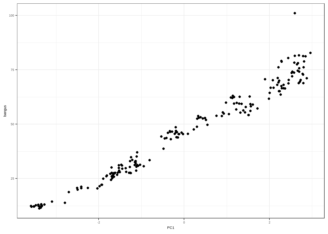
Limitation of PCR: model interpretation may be difficult.
More details about the theory of variable reduction and the Principal Component Analysis in Stat 147. Here in Stat 136, it is not recommended that you use this in your paper.
Exercise
Exercise 12.2 Using the bangus dataset and the model containing all possible independent variables in the dataset, show the VIF, condition indices, and variance proportions for detecting multicollinearity. Interpret the results.
Other References
- Liao, D., & Valliant, R. (2012). Condition Indexes and Variance Decompositions for Diagnosing Collinearity in Linear Model Analysis of Survey Data. Survey Methodology, 1–19. https://www.rti.org/publication/condition-indexes-and-variance-decompositions-diagnosing-collinearity-linear-model/fulltext.pdf