CHAPTER 2 Introduction to Regression and Linear Models

Regression Analysis is a statistical tool that utilizes the relation between a dependent variable and one or more independent variables so that the dependent variable can be predicted using the independent variable/s.

In this course, we will focus on datasets and models where the dependent and independent variables are numeric or quantitative in nature.

---

2.1 Historical Origin of the term “Regression”

• Regression analysis was first developed by Sir Francis Galton in the latter part of the 19th century.

  

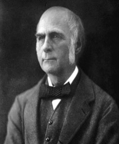
• Galton had studied the heights of fathers and sons and noted that the heights of sons of both tall and short fathers appeared to revert or regress to the mean of height of the fathers. He considered this tendency to be a regression to mediocrity.

• Galton developed a mathematical description of this regression tendency, the precursor of today’s regression models.

• The term regression persists to this day to describe statistical relations between variables, but may be differently described from how Galton first used it.

• Most of the statistical methodologies pioneered by Galton (regression, psychometrics, usage of questionnaires) are unfortunately utilized by Galton for eugenics and scientific racism.

---

2.2 Uses of Regression Analysis

• Data Description – summarize and describe the data; describes the relationship of the dependent variable against the independent variable
• Prediction – forecast the expected value of the variable of interest given the values of the other (independent) variables; very important and useful in planning
• Structural Analysis – the use of an estimated model for the quantitative measurement of the relationships of the variables (example: economic variables); it facilitates the comparison of rival theories of the same phenomena; quantifies the relationship between the variables

---

2.3 Classification of Regression Models

In terms of distributional assumptions

• Parametric – assumes a fixed structural form where the dependent variable (linearly) depends on the independent variables; the distribution is known and is indexed by unknown parameters
• Nonparametric – the dependent variable depends on the explanatory variables but the distribution is not specified (distribution-free) and not indexed by a parameter
• Semi-parametric – considers an unknown distribution but indexed by some parameter

In terms of types of dependent and independent variables

Dependent	Independent	Model
Continuous	Continuous	Classical Regression
Continuous	Continuous added Categorical	Classical Regression with use of Dummy Variables
Continuous	Categorical added Continuous	Analysis of Covariance (ANCOVA)
Continuous	All Categorical	Analysis of Variance (ANOVA)
Categorical	Any Combination	Logistic Regression
Categorical	All Categorical	Log-Linear Models

---

2.4 The Linear Model

Two points can be represented by a straight line. Recall the slope-intercept equation of a line

$$Y = a + mX$$

where $a$ is the y-intercept, and $m$ is the slope of the line.

---

Example 1: Some deterministic models can be represented by a straight line.

You are selling hotdogs with a unit price of 25 pesos per piece. Assuming there are no tips and you have no other items to sell, then the daily sales has a deterministic relationship with the number of hotdogs sold.

$$sales =25 \times hotdogs$$

However, most phenomena are governed by some probability or randomness. What if we are modelling the expected net income where we consider the tips, possible spoilage of food, and other random scenario?

That is why we add a random error term $\varepsilon$ to characterize a stochastic linear model.

$$sales = 25 \times hotdogs + \varepsilon$$ where $\varepsilon$ is a random value that may be positive or negative.

---

Example 2: a variable can be a function of another variable, but the relationship may be stochastic, not deterministic.

Suppose we have the following variables collected from 10 students.

student <- read.csv("student.csv")

• $X$ - highschool exam score in algebra
• $Y$ - Stat 101 Final Exam scores

Student	X	Y
1	90	85
2	87	87
3	85	89
4	85	90
5	95	92
6	96	94
7	82	80
8	78	75
9	75	60
10	84	78

 

 

There seems to be a linear relationship between $X$ and $Y$ (although not perfectly linear).

Our main goal is to represent this relationship using an equation.

 

In this graph:

• $Y = \beta_0 + \beta_1X$ represents the straight line.
• $Y_i = \beta_0 + \beta_1X_i+\varepsilon_i$ represents the points in the scatter plot
• The $\beta$s are the model parameters
• The $\varepsilon$s are the error terms

• If we are asking “which equation best represents the data”, it is the same as asking “what are the values of $\beta$ that best represent the data”.
• If there are $k$ independent variables, the points are represented by: $Y_i = \beta_0 + \beta_1X_{i1} + \beta_2X_{i2} + \cdots + \beta_kX_{ik} + \varepsilon_i$

Justification of the Error Term

• The error term represents the effect of many factors (apart form the X’s) not included in the model which do affect the response variable to some extent and which vary at random without reference to the independent variables.
• Even if we know that the relevant factors have significant effect on the response, there is still a basic and unpredictable element of randomness in responses which can be characterized by the inclusion of a random error term.
• $\varepsilon$ accounts for errors of observations or measurements in recording $Y$.
• Errors can be positive or negative, but are expected to be very small (close to 0)

Linear Model in Matrix Form

Take note that we assume a model for every observation $i=1,\cdots, n$, which implies that we are essentially handling $n$ equations. To facilitate handling n equations, we can use the concepts in matrix theory.

Instead of $Y_i = \beta_0 + \beta_1X_{i1} + \beta_2X_{i2} + \cdots + \beta_kX_{ik} + \varepsilon_i$ for each observation $i$ from $1$ to $n$, we can make it compact using matrix notations.

Given the following vectors and matrices:

$$\textbf{Y}=\begin{bmatrix} Y_1 \\ Y_2 \\ \vdots\\ Y_n \end{bmatrix} \quad \textbf{X} =\begin{bmatrix} 1 & X_{11} & X_{12} & \cdots & X_{1k} \\ 1 & X_{21} & X_{12} & \cdots & X_{2k} \\ \vdots & \vdots & \vdots & \ddots & \vdots \\ 1 & X_{n1} & X_{n2} & \cdots & X_{nk} \end{bmatrix} \quad \boldsymbol{\beta}= \begin{bmatrix} \beta_0 \\ \beta_1 \\ \beta_2 \\ \vdots\\ \beta_k \end{bmatrix} \quad \boldsymbol{\varepsilon} = \begin{bmatrix} \varepsilon_1 \\ \varepsilon_2 \\ \vdots\\ \varepsilon_n \end{bmatrix}$$

Definition 2.1 (Matrix Form of the Linear Equation)
The $k$-variable, $n$-observations linear model can be written as

$$\begin{align} \underset{n\times1}{\textbf{Y}} &= \underset{n\times (k+1)}{\textbf{X}}\underset{(k+1)\times1}{\boldsymbol{\beta}} + \underset{n\times 1}{\boldsymbol{\varepsilon}}\\ \\ \begin{bmatrix} Y_1 \\ Y_2 \\ \vdots\\ Y_n \end{bmatrix} &= \begin{bmatrix} 1 & X_{11} & X_{12} & \cdots & X_{1k} \\ 1 & X_{21} & X_{12} & \cdots & X_{2k} \\ \vdots & \vdots & \vdots & \ddots & \vdots \\ 1 & X_{n1} & X_{n2} & \cdots & X_{nk} \end{bmatrix} \begin{bmatrix} \beta_0 \\ \beta_1 \\ \beta_2 \\ \vdots\\ \beta_k \end{bmatrix} + \begin{bmatrix} \varepsilon_1 \\ \varepsilon_2 \\ \vdots\\ \varepsilon_n \end{bmatrix} \\ \\ \begin{bmatrix} Y_1 \\ Y_2 \\ \vdots\\ Y_n \end{bmatrix} &= \begin{bmatrix} \beta_0 + \beta_1X_{11} + \beta_2X_{12} + \cdots & \beta_kX_{1k} +\varepsilon_1 \\ \beta_0 + \beta_1X_{21} + \beta_2X_{12} + \cdots & \beta_kX_{2k} +\varepsilon_2\\ \vdots \\ \beta_0 + \beta_1X_{n1} + \beta_2X_{n2} + \cdots & \beta_kX_{nk} +\varepsilon_n \end{bmatrix} \end{align}$$

where

• $Y_i$ is the value of the response variable on the $i^{th}$ trial. Collectively, $\textbf{Y}$ is the response vector.
• $X_{ij}$ is a known constant, namely, the value of the $j^{th}$ independent variable on the $i^{th}$ trial. Collectively, $\textbf{X}$ is the design matrix.
• $\beta_0, \beta_1, \cdots , \beta_k$ are parameters. Collectively, $\boldsymbol{\beta}$ is the regression coefficients vector.
• $\varepsilon_i$ is a random error term on trial $i=1,...,n$. Collectively, $\boldsymbol{\varepsilon}$ is the error term vector.

The statistical uses of the linear model:

• The model summarizes the linear relationship between $Y$ and the $X$ s.
• It can help explain how variability in $Y$ is affected by the $X$ s.
• It can help determine $Y$ given prior knowledge on $X$ .

Illustrations for the Case of 2 Independent Variables

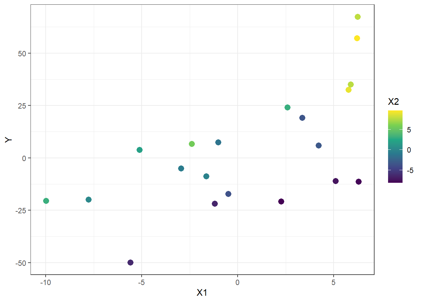
Suppose you have the following dataset:

Y	X1	X2
34.2100651	9.9990548	-6.0040036
-14.1264391	9.8777310	-9.0847566
-32.2461207	-9.7716595	1.9321054
-10.7948056	-9.6845970	1.6714682
-0.9478368	6.3352737	-9.0131671
1.4818877	2.9240957	-2.3861465
57.8052390	9.8140187	6.6935443
-15.3143807	8.6622348	-9.2594677
-18.6425027	-5.7757841	-0.5062797
-29.7737151	-3.4454354	-6.0677981
4.8287906	2.6305855	2.9518126
-4.0625759	-2.6867529	-1.0129115
-7.8535094	-8.0157701	1.5578754
33.9705132	0.4840261	8.5812561
1.2334292	4.8936139	-8.8063998
8.8035582	-1.8554113	-0.6839487
10.0313699	3.0492480	1.6572168
-5.2238779	-7.1827343	5.8523271
-8.6736718	1.5886260	-7.0121909
-45.2719876	-5.9297143	-7.9327379

In a 2-dimensional plane, it can be visualized as follows

It can be also visualized using a 3-dimensional plane. You can drag around to change the view angle.

Now, we want a line (or a sheet) that passes through the center of the points. Let’s try this equation: $$Y = 2 + 3X_1 + 4X_2$$ The line that passes through the center of the points can be visualized in this 3D graph:

---

2.5 Assumptions

The multiple linear regression model is represented by the matrix equation $\textbf{Y} = \textbf{X} \boldsymbol{\beta} + \boldsymbol{\varepsilon}$

Given $n$ observations, we want to fit this equation.

How do we regulate the balance between summarizing data and model fit?

 

IMPOSE ASSUMPTIONS

Types of Error Assumptions

• Classical Assumptions: $E(\varepsilon_i)=0 ,\quad Var(\varepsilon_i)=\sigma^2 \quad\forall i, \quad Cov(\varepsilon_i,\varepsilon_j)=0 \quad \forall i\neq j$

• Normal Error Model Assumptions: $\varepsilon_i\overset{iid}{\sim}N(0,\sigma^2)$

Linear Regression Variable Assumptions

• Independent Variables: Assumed to be constant, predetermined, or something that is already gathered; uncorrelated (definitely not related with the error terms).

• Dependent Variable: Assumed to still be unknown and inherently random; independent with one another.

Important Features of the Model

1. ($Y_i$ as a random variable). The observed value of $Y_i$ in the $i^{th}$ trial is the sum of two components: $$Y_i\quad=\quad\underset{\text{constant terms}}{\underbrace{\beta_0 + \beta_1X_{i1} + \beta_2X_{i2} + \cdots + \beta_kX_{ik}}} \quad+ \underset{\text{random term}}{\underbrace{\varepsilon_i}}$$

   Hence, $Y_i$ is a random variable.

2. (Expectation of $Y_i$). Since $E(\varepsilon_i) = 0$, it follows that $E(Y_i)=\beta_0 + \beta_1X_{i1} + \beta_2X_{i2}+ \cdots + \beta_kX_{ik}$. Thus, the response $Y_i$, when the level of the $k$ independent variables (X’s) in the $i^{th}$ trial are known, comes from a probability distribution whose mean is $\beta_0 + \beta_1X_{i1} + \beta_2X_{i2}+ \cdots + \beta_kX_{ik}$. This constant value is referred to as the regression function for the model.

3. (Error Term). The observed value of the $Y_i$ in the $i^{th}$ trial exceeds or falls short of the value of the regression function by the error term amount $\varepsilon_i$.

4. (Homoscedasticity). The error terms are assumed to have a constant variance. Thus, the responses $Y_i$ have the same constant variance.

5. (Independence of Observations). The error terms are assumed to be uncorrelated. Hence, the outcome in any one trial has no effect on the error term for any other trial – as to whether it is positive or negative, small or large. Since the error terms $\varepsilon_i$ and $\varepsilon_j$ are uncorrelated, so are the responses $Y_i$ and $Y_j$.

6. (Distribution of $Y_i$). The assumption of normality of error terms implies that the $Y_i$ are also independent (but not necessarily identical) normal random variables. That is: $$Y_i\overset{ind}{\sim}Normal(\mu=\beta_0 + \beta_1X_{i1} + \beta_2X_{i2}+ \cdots + \beta_kX_{ik},\sigma^2)$$

   Is it justifiable to impose normality assumption on the error terms?

   • A major reason why the normality assumption for the error terms is justifiable in many situations is that the error terms frequently represent the effects of many factors omitted explicitly in the model, that do affect the response to some extent and that vary at random without reference to the independent variables. Also, there might be random measurement errors in recording $Y$.
     • Insofar as these random effects have a degree of mutual independence, the composite error term representing all these factors will tend to comply with the CLT and the error term distribution would approach normality as the number of factor effects becomes large.
       
   • A second reason why the normality assumption for the error terms is frequently justifiable is that some of the estimation and testing procedures to be discussed in the next chapters are based on the t-distribution, which is not sensitive to moderate departures from normality.
     • Thus, unless the departures from normality are serious, particularly with respect to skewness, the actual confidence coefficients and risks of errors will be close to the levels for exact normality.

In summary, the regression assumptions are the following:

• the expected value of the unknown quantity $\varepsilon_i$ is 0 for every observation $i$
  
• the variance of the errors term is the same for all observations
  
• the error terms and observations are uncorrelated
  
• the error terms follow a normal distribution
  
• the independent variables are not strongly correlated to each other

2.6 Introduction: The Multivariate Normal

This is just a quick introduction. Theory and more properties will be discussed in Stat 147.

If we are going to use the normal Error assumption in our regression models, knowledge of the multivariate normal random variable is important.

Definition 2.2 (Multivariate Normal)

Let $\boldsymbol{\mu}\in \mathbb{R}^n$ and let $\boldsymbol{\Sigma}$ be a $n\times n$ positive semidefinite matrix as defined in Equations (1.1) and (1.2) respectively.

The $n\times 1$ vector $\boldsymbol{Y}$ is said to have a multivariate distribution with parameters $\boldsymbol{\mu}$ and $\boldsymbol{\Sigma}$, written as $\boldsymbol{Y}\sim N_n(\boldsymbol{\mu}, \boldsymbol{\Sigma})$, if and only if $\boldsymbol{l}'\boldsymbol{Y}\sim N(\boldsymbol{l}'\boldsymbol{\mu}, \boldsymbol{l}'\boldsymbol{\Sigma}\boldsymbol{l})$ for every $n\times 1$ vector $\boldsymbol{l}$.

The definition simply states that for $\boldsymbol{Y}$ to be multivariate normal, every linear combination of its components must be univariate normal with parameters $\boldsymbol{l}'\boldsymbol{\mu}$ and $\boldsymbol{l}'\boldsymbol{\Sigma}\boldsymbol{l}$.

$$l_1Y_1+l_2Y_2+\cdots+l_nY_n\sim N(\boldsymbol{l}'\boldsymbol{\mu}, \boldsymbol{l}'\boldsymbol{\Sigma}\boldsymbol{l})$$

Properties of the Multivariate Normal

If $\boldsymbol{Y}\sim N_p(\boldsymbol{\mu},\boldsymbol{\Sigma})$, then the following properties hold:

1. The mean and variance of $\bf{x}$ are $E(\boldsymbol{Y})=\boldsymbol{\mu}$ and $V(\boldsymbol{Y})=\boldsymbol{\Sigma}$.

2. For any vector of constants $\boldsymbol{a}$, $\boldsymbol{Y}+\boldsymbol{a} \sim N(\boldsymbol{\mu}+\boldsymbol{a}, \boldsymbol{\Sigma})$

3. The marginal distributions of the components are univariate normal, i.e. $Y_i \sim N(\mu_i, \sigma_{ii})$, $i=1,...,n$, where $\mu_i$ and $\sigma_{ii}$ are the mean and variance respectively of component $Y_i$.

4. For two components $Y_i$ and $Y_j$, $i\neq j$, their covariance can be found on the off-diagonal elements of $\boldsymbol{\Sigma}$, i.e. $cov(Y_i,Y_j)=\sigma_{ij}$

5. If $\textbf{L}$ is a $(p \times n)$ matrix of rank $p$, then $\textbf{L}\boldsymbol{Y}\sim N_p(\textbf{L}\boldsymbol{\mu}, \textbf{L}\boldsymbol{\Sigma}\textbf{L}')$

6. The joint PDF of $\boldsymbol{Y}$ is given by $$f_\boldsymbol{Y}(\boldsymbol{y})=\frac{1}{(2\pi)^{n/2}|\boldsymbol{\Sigma}|^{1/2}} \exp\left\{-\frac{1}{2} (\boldsymbol{y}-\boldsymbol{\mu})'\boldsymbol{\Sigma}^{-1}(\boldsymbol{y}-\boldsymbol{\mu})\right\},\quad \boldsymbol{y} \in \mathbb{R}^n$$

Questions:

1. If two random variables are independent, are they uncorrelated?

   Answer

   Yes.

2. If two random variables are uncorrelated, are they independent?

   Answer

   Generally, No. But if they are normally distributed, then Yes.

   This implies that if $\boldsymbol{Y}\sim N(\boldsymbol{\mu},\boldsymbol{\Sigma})$ where $\boldsymbol{\Sigma}=\text{diag}(\sigma^2_1, \sigma^2_2,\cdots,\sigma^2_n)$, then the marginals are mutually independent to each other, i.e. $Y_1,Y_2,\cdots Y_n \overset{Ind}{\sim} N(\mu_i,\sigma^2_i)$.

3. For a multivariate random vector $\boldsymbol{Y}=\begin{bmatrix} Y_1 & Y_2& \cdots & Y_n \end{bmatrix}'$, if the marginal components are all univariate normal, i.e. $Y_i\sim N(\mu_i, \sigma_{ii})$ for all $i$, then does this imply that $\boldsymbol{Y}$ follows a multivariate normal distribution?

   Answer

   No. Not necessarily.

   The problem with this question is that the mean vector and covariance matrix are not defined.

   As a counter example, suppose $\boldsymbol{Y}=\begin{bmatrix} Y_1 & Y_2 \end{bmatrix}'$ has a joint PDF

   $$f_\boldsymbol{Y}(\boldsymbol{y}) = \frac{1}{2\pi}e^{-\frac{1}{2}(y_1^2+y_2^2)}\times\left[1+ y_1y_2 e^{-\frac{1}{2}(y_1^2+y_2^2)} \right],\quad \boldsymbol{y} \in \mathbb{R}^2$$ This is NOT the pdf of a bivariate normal. Therefore, $\boldsymbol{Y}$ does not follow a multivariate normal distribution.

   However, if we derive the marginal distributions of $Y_1$ and $Y_2$, we will obtain univariate normal PDFs.

   Proof:

   $$\begin{align} f_{Y_1}(y_1) &= \int_{-\infty}^\infty f(\boldsymbol{y})dy_2 \\ &=\int_{-\infty}^\infty \frac{1}{2\pi}e^{-\frac{1}{2}(y_1^2+y_2^2)}\times\left[1+ y_1y_2 e^{-\frac{1}{2}(y_1^2+y_2^2)} \right] dy_2\\ &= \underbrace{\int_{-\infty}^\infty \frac{1}{2\pi}e^{-\frac{1}{2}(y_1^2+y_2^2)} dy_2}_{(a)} + \underbrace{\int_{-\infty}^\infty \frac{1}{2\pi}e^{-\frac{1}{2}(y_1^2+y_2^2)}y_1y_2 e^{-\frac{1}{2}(y_1^2+y_2^2)}dy_2}_{(b)} \end{align}$$

   Aside (a):

   $$\begin{align} (a) &= \frac{1}{\sqrt{2\pi}}e^{-\frac{1}{2}y_1^2}\int_{-\infty}^\infty \underbrace{\frac{1}{\sqrt{2\pi}}e^{-\frac{1}{2}y_2^2}}_{\text{pdf of } N(0,1)} dy_2\\ &= \frac{1}{\sqrt{2\pi}}e^{-\frac{1}{2}y_1^2} \end{align}$$ Aside (b):

   $$\begin{align} (b) &= \int_{-\infty}^\infty \frac{1}{2\pi}y_1y_2 e^{-(y_1^2+y_2^2)}dy_2\\ &=\int_{-\infty}^\infty \frac{1}{2\pi}y_1 e^{-y_1^2} y_2 e^{-y_2^2}dy_2\\ &=\frac{1}{2\pi}y_1 e^{-y_1^2}\int_{-\infty}^\infty y_2 e^{-y_2^2}dy_2 \\ &= \frac{1}{2\pi}y_1 e^{-y_1^2}\left(-\frac{e^{-y_2^2}}{2} \Biggm|_{x_2=-\infty}^{x_2=+\infty}\right) \\ &= \frac{1}{2\pi}y_1 e^{-y_1^2}(0-0) \\ &=0 \end{align}$$ Therefore, the marginal pdf of $Y_1$ is

   $$f_{Y_1}(y_1)=\frac{1}{\sqrt{2\pi}}e^{-\frac{1}{2}y_1^2}$$ which is a univariate $Normal(0,1)$.

   Using the same process, we can also see that $Y_2\sim N(0,1)$

   Therefore, we showed a multivariate random vector that DOES NOT follow the multivariate normal distribution, but has marginal components that each has univariate normal PDFs.

   Having univariate normal as marginal distributions does not imply that the joint distribution is multivariate normal. $\blacksquare$

Implications for the Normal Error Assumption

Recall our assumptions for the error term:

• the expected value of the unknown quantity $\varepsilon_i$ is 0 for every observation $i$

• the variance of the errors term is the same for all observations

• the error terms are independent from each other

• the error terms follow a normal distribution

In other words, $\varepsilon_1, \varepsilon_2, \cdots, \varepsilon_n \overset{iid}{\sim}N(0,\sigma^2)$

We can express it as a random vector of errors $\boldsymbol{\varepsilon}=\begin{bmatrix} \varepsilon_1 & \varepsilon_2 & \cdots & \varepsilon_n \end{bmatrix}'$, and its distribution is assumed to be $n$-variate normal. That is,
$$\boldsymbol{\varepsilon} \sim N_n(\textbf{0},\sigma^2\textbf{I})$$

---

© 2024 Siegfred Roi Codia. All rights reserved.