Chapter 10 Nonnormality and Heteroskedasticity
This is part 2 of the diagnostic checking.
Recall the assumption about the random error term: \[ \varepsilon_i\sim Normal(0,\sigma^2) \]To test assumptions about the error term, we explore the characteristic of the residuals instead
In this section, we want to know if the residuals are sampled from a normally distributed population and has the same variance regardless of the valuue of \(Y_i\).
10.1 On Nonnormality
Reasons of Nonnormality
- Existence of outliers in the model (nonsystematic problem).
- There are still too much variability of Y that is due to error (systematic problem).
- Relationship of the regressors with the dependent variable is nonlinear (systematic problem).
- \(Y\) is inherently far from being normally distributed (systematic problem).
Implications of Nonnormality
Note that the several of the tests and procedures we have discussed assume normality of error terms.
The tests and confidence intervals for the model parameters assume normality of the error terms
Recall Section 6.1
Additionally, the prediction of new responses assumes normality of the error terms.
Recall Section 6.3
The rationale behind the MSE being the UMVUE for the error term variance also assumes normality.
Recall Theorem 4.16
However, take note that the \(\hat{\boldsymbol{\beta}}\) being the BLUE of \(\boldsymbol{\beta}\) does not require the assumption of normality of error terms. Recall Theorem 4.14
Note also of the fact that because of the central limit theorem, a lot of statistics used for hypothesis testing and confidence interval estimation approximately follows the normal distribution.
Given these realities, many statisticians have stated that the assumption of normality is the least troublesome among the assumptions of regression analysis. However, it remains essential to check for significant deviations from normality.
Graphical Tools for Detecting Nonnormality
Useful graphical tools for assessing the normality of a given variable are histograms (with super-imposed normal curve) and normal probability plots.
Histogram
library(carData)
data(Anscombe)
mod_anscombe <- lm(income ~ education + young + urban, data = Anscombe)
olsrr::ols_plot_resid_hist(mod_anscombe)
You can manually create histograms using ggplot.
library(ggplot2)
ggplot(data.frame(resid = resid(mod_anscombe)),
                aes(x = resid)) +
    geom_histogram(aes(y=..density..), bins = 10) + theme_bw()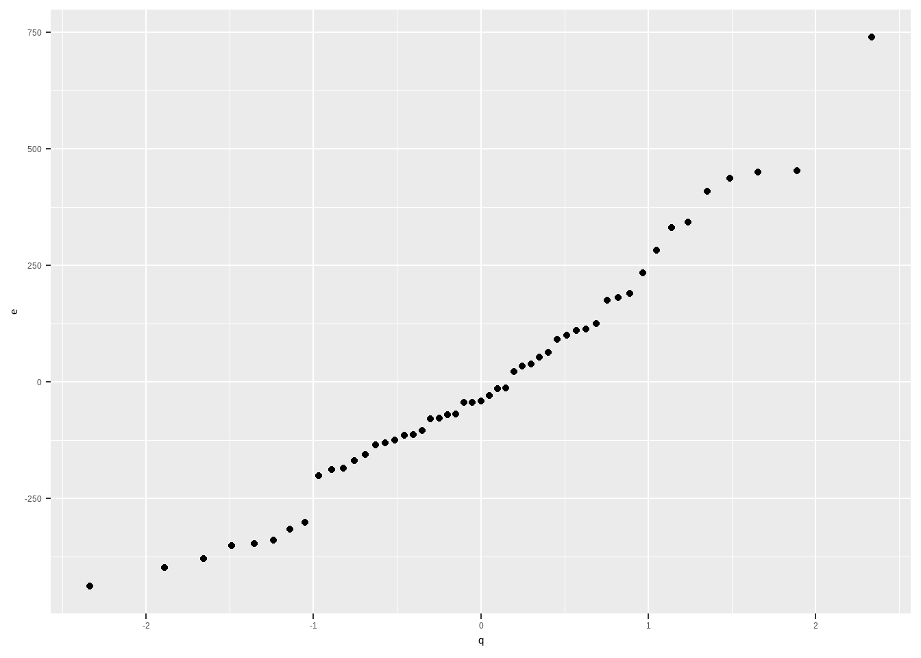
Normal Probability Plots
In general, this is called the Quantile-Quantile Plot, but for normal distribution.
We plot on y-axis the residuals (can be standardized) and then we plot on the x-axis the theoretical quantiles of the residuals if we assume that it follows the normal distribution.
The following summarizes the steps in creating a normal probability plot:
- Let \(e_{(1)}<e_{(2)}<\cdots<e_{(n)}\) be the residuals ranked in increasing order.
- Calculate the empirical cumulative probabilities as \(p_i=\frac{i-0.5}{n}\)
- Compute theoretical quantiles of each \(e_{(i)}\) as \(\Phi^{-1}(p_i)\), where \(\Phi\) is the cdf of a standard normal distribution.
- Plot the residuals on the y-axis, and the theoretical quantiles on the x-axis.
The resulting scatter plot should look like a straight line. Substantial departures from a straight line indicate that the distribution is not normal.
The straight line is usually determined visually, with emphasis on the central values rather than the extremes.
e     <- resid(mod_anscombe)
p     <- (rank(e)-0.5)/length(e)
q     <- qnorm(p)

data.frame(e,q) |>
    ggplot(aes(x = q, y = e))+
    geom_point()
But sometimes, the standardized residuals is used so the scatter plot can be easily compared to the diagonal line \(y=x\)
# standardized residuals
std.e <- rstandard(mod_anscombe)

data.frame(std.e,q) |>
    ggplot(aes(x = q, y = std.e))+
    geom_point() + geom_abline(slope=1) +
    xlim(-2.5, 3) + ylim(-2.5, 3)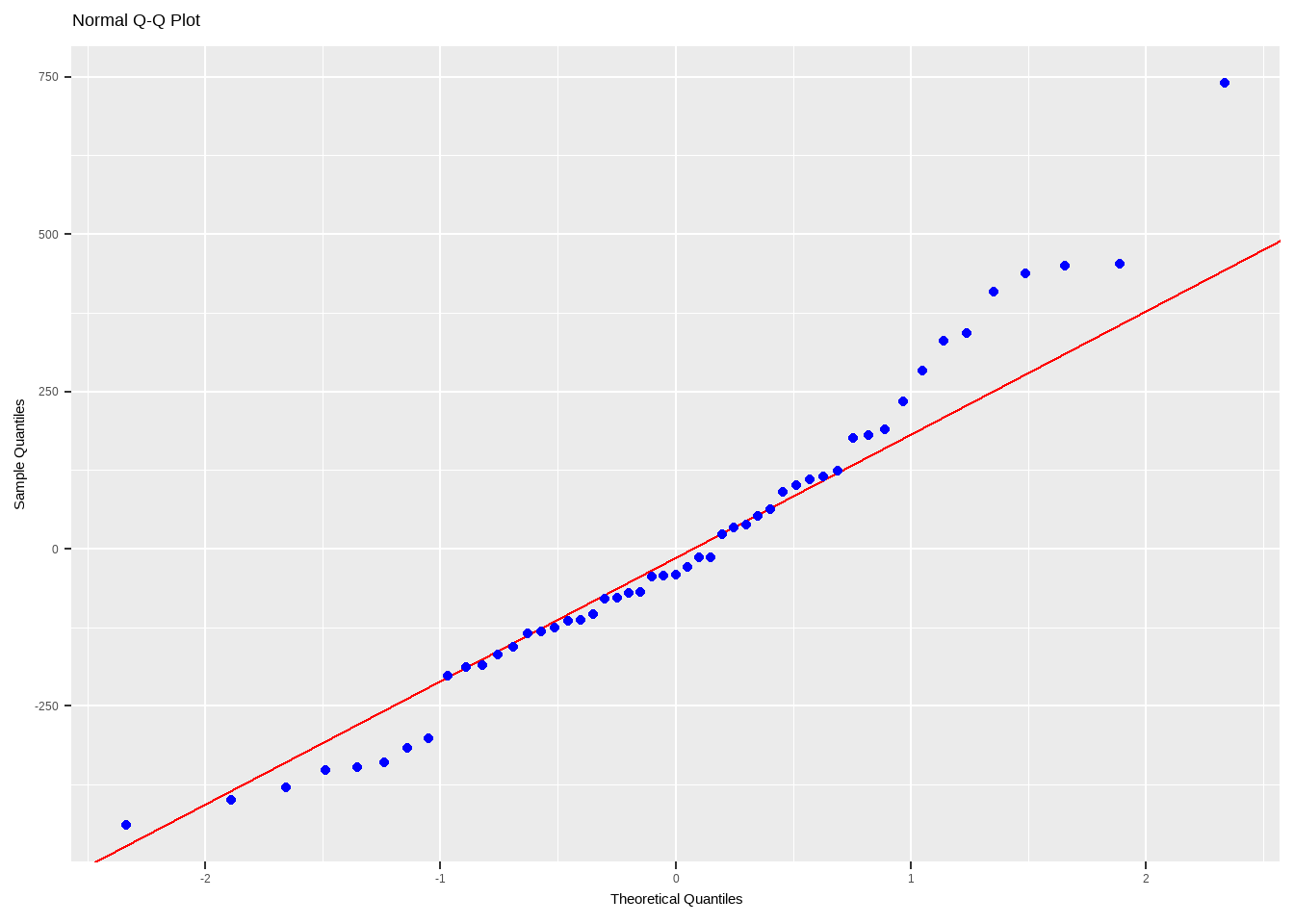
The codes above are just to explain how to construct a Q-Q plot manually. There are ready functions you can use to show the Normal Probability Plots.

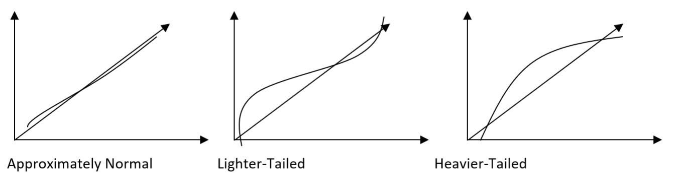
Interpreting the Normal Probability Plot
Remarks:
- Small sample sizes (n ≤ 16) often produce normal probability plots that deviate substantially from the diagonal line.
- For large sample sizes (n ≥ 32), the plots are much better behaved.
- Usually about 20 points are required to produce normal probability plots that are stable enough to be easily interpreted.
- A common defect that shows up on the normal probability plot is the occurrence of one or two large residuals. These can be found at the either end of the qq plot, and may largely deviate from the straight line. Sometimes, this is an indication that the corresponding observations are outliers.
Testing for Nonnormality
\[\begin{align} Ho:& \text{ the error terms are normally distributed}\\ Ha: & \text{ the error terms are not normally distributed} \end{align}\]
The following are some of the tests that may be used for validating the assumption of normality of the error terms.
\(\chi^2\) Goodness-of-fit-test
Description: The interest is in the number of subjects or objects that fall in various categories. In the \(\chi^2\) goodness-of-fit test, we wish to test whether a significant difference exists between an observed number of objects in a category and an expected number of observations based on the null hypothesis. (This is discussed in full in Stat 132)
Strengths: A very intuitive test. Easy to visualize using histogram.
Weaknesses: The test is very sensitive to the binning process. There is also a requirement for the expected frequencies per bin (≥ 5).
##
##  Pearson chi-square normality test
##
## data:  resid(mod_anscombe)
## P = 8.8039, p-value = 0.267
Kolmogorov-Smirnov One-Sample Test
Also called “Lilliefors Test”
Description: This is another goodness-of-fit test that is concerned with the degree of agreement between the distribution of a set of observed scores and some specified distribution (This is discussed in full in Stat 132).
Strengths: It is not sensitive to departure from other assumptions. It is also not sensitive to several identical values.
Weaknesses: It is less powerful than most tests for normality. It requires larger sample size being a nonparametric test.
The following R codes performs the Lilliefors test. While the test statistic are the same, p-values may be different, since assumed sampling distribution are different in the two functions.
## ## Exact one-sample Kolmogorov-Smirnov test ## ## data: resid(mod_anscombe) ## D = 0.090582, p-value = 0.7628 ## alternative hypothesis: two-sided## ## Lilliefors (Kolmogorov-Smirnov) normality test ## ## data: resid(mod_anscombe) ## D = 0.090582, p-value = 0.3709
Shapiro-Wilk test
Description: A test that essentially looks at the correlation between the ordered data and the theoretical values from thenormal distribution.
Strengths: This is one of the most powerful normality-tests. It is also one of the most popular tests too. One can use it for small sample sizes.
Weaknesses: It being a very powerful test is a problem in itself, especially if the sample size is too large. If the sample size is sufficiently large this test may detect even trivial departures from the null hypothesis (for example: outlying residuals). The test is also very sensitive to many identical residual values.
##
##  Shapiro-Wilk normality test
##
## data:  resid(mod_anscombe)
## W = 0.96789, p-value = 0.1805
Cramér-von Mises criterion
Description: In statistics the Cramer-von-Mises criterion for judging the goodness-of-fit of a probability distribution \(F^∗(x)\) compared to a given distribution \(F\) is given by
\[ W^2=\int_{-\infty}^{\infty}[F(x)-F^*(x)]^2dF(x) \]
In applications, \(F(x)\) is the theoretical distribution and \(F^∗(x)\) is the empirically observed distribution.
Strengths: This is a nonparametric test, which implies that it is a robust test. It is also more powerful than Kolmogorov-Smirnov Test.
Weaknesses: It is not as powerful as Shapiro-Wilk and Anderson-Darling. It is also very sensitive to observation ties.
##
##  Cramer-von Mises normality test
##
## data:  resid(mod_anscombe)
## W = 0.073021, p-value = 0.25
Anderson-Darling Test
Description: This is a test that compares the quantile values of the empirical distribution of the data with the theoretical distribution of interest. It is based upon the concept that when given a hypothesized underlying distribution, the data can be transformed to a uniform distribution.
Strengths: The Anderson-Darling test is one of the most powerful statistics for detecting most departures from normality. It may be used with small sample sizes, n ≤ 25.
Weaknesses: Very large sample sizes may reject the assumption of normality with only slight imperfections, but industrial data with sample sizes of 200 and more have passed the Anderson-Darling test. The test is also very sensitive to many identical residual values
##
##  Anderson-Darling normality test
##
## data:  resid(mod_anscombe)
## A = 0.46164, p-value = 0.2486
Jarque-Bera Test
In statistics, the Jarque-Bera test is a goodness-of-fit measure of departure from normality, based on the sample kurtosis and skewness. The test statistic JB is defined as
\[ JB=\frac{n}{6}\left(S^2 +\frac{(K-3)^2}{4} \right) \]
where \(n\) is the number of observations (or degrees of freedom in general); \(S\) is the sample skewness; and \(K\) is the sample kurtosis.
The statistic JB has an asymptotic chi-square distribution with two degrees of freedom and can be used to test the null hypothesis that the data are from a normal distribution. The null hypothesis is a joint hypothesis of both the skewness and excess kurtosis being 0, since samples from a normal distribution have an expected skewness of 0 and an expected excess kurtosis of 0. As the definition of JB shows, any deviation from this increases the JB statistic.
Illustration in R
## -----------------------------------------------
##        Test             Statistic       pvalue
## -----------------------------------------------
## Shapiro-Wilk              0.9679         0.1805
## Kolmogorov-Smirnov        0.0906         0.7628
## Cramer-von Mises          4.4902         0.0000
## Anderson-Darling          0.4616         0.2486
## -----------------------------------------------
Exercise 10.1 Summarize the mentioned tests for normality. Create a table that shows the following for each test:
- definition
- the test statistic and sampling distribution (if applicable)
- assumptions
- advantages - when best to use, how is it better than the other tests?
- weaknesses - when not to use, how is it worse than the other tests?
- Other details, such as relationship of each test to each other.
Only use descriptions given here as guide. Do not directly quote them. Instead, use other references. Do not forget to cite your sources.
10.2 On Heteroskedasticity
One of the assumptions of the regression model is that the variation of the error terms is everywhere the same. Heteroskedasticity is the problem of having nonconstant variances of the error terms.
If this problem is present, the residual plots are usually funnel-shaped or diamond-shaped.
A common reason for this is that the dependent variable Y follows a probability distribution in which the variance is functionally related to the mean.
- It is important to detect and correct a nonconstant error variance.
- If this problem is not eliminated, the least squares estimators will still be unbiased, but they will no longer have the minimum variance property.
- This means that the regression coefficients will have larger standard errors than necessary.
Reasons for Heteroskedasticity
Heteroskedasticity arises when…
The variability is a function of the variable themselves.
Example 1: Basketball Points
In a basketball league, if \(X\) represents playing time per game and \(Y\) represents points scored per game, players who stay on the court longer tend to score more, but their point totals also show greater variability, since other factors influence performance. Some players may log heavy minutes because of their defensive strengths rather than scoring ability.
This example will produce fan-shaped heteroskedasticity.

See case (ii) in Interpretation of Residual Plots.
Example 2: Income and Expenditure
As income grows, people have more discretionary income and hence more scope of choice about the disposition of their income; variance of expenditure is expected to increase with income
Same with the first example, this will also produce a fan-shaped heteroskedasticity.There is presence of outliers
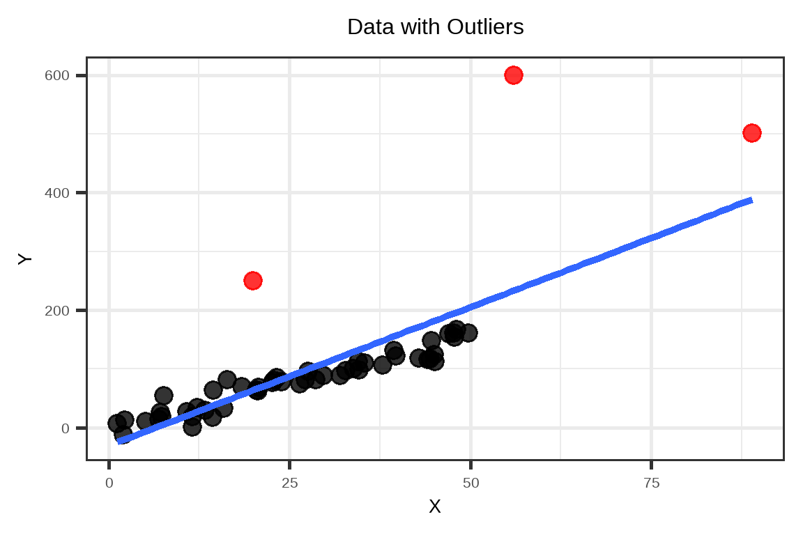
Example: Data with outliers
Outliers will increase the spread of residuals, creating heteroskedasticity even if the relationship is otherwise linear. Suppose we have the following dataset.

The outliers “pull” the fitted regression line away from the general trend of the other observations. This will result to the following fitted vs residual plot.
 As you can see, the residuals \(e\) of the majority of the observations have a decreasing trend with respect to the fitted values \(\hat{Y}\).
See case (iii) in Interpretation of Residual Plots.
The regression model is incorrectly specified
Example: A Quadratic Model
Suppose the true model is
\[ Y = -3X + 0.2X^2+\varepsilon, \quad \varepsilon \sim N(0,1) \]
But you fit
\[ Y = \beta_0 + \beta_1 X + u \]
Because the model “forces a straight line” through a curved relationship, it produces a nonlinear or quadratic heteroskedasticity.
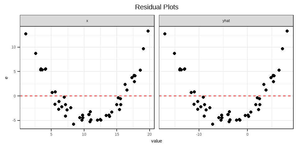
See case (iv) in Interpretation of Residual Plots.
Implications of Heteroskedasticity
Under heteroskedasticity, while Ordinary Least Squares (OLS) estimators remain linear and unbiased, but their reliability is compromised instead.
- Since we require the assumption that \(Var(\boldsymbol\varepsilon) = \sigma^2\textbf{I}\) for Gauss-Markov Theorem and the derivation of the UMVUE, OLS estimators are not efficient when \(Var(\boldsymbol\varepsilon) \neq \sigma^2\textbf{I}\) .
- The OLS estimators are no longer BLUE and UMVUE.
- Moreover, they are also not asymptotically efficient, or they do not become efficient even if the sample size increases.
Most implications are almost the same if nonnormality occurs: assumptions of the statistical tests will also be violated.
- We also required the assumption of constancy of variance to derive the ANOVA F-test. This test is misleading if we have a problem of heteroskedasticity.
- Variance of \(\hat{\boldsymbol{\beta}}\) is no longer equal to \(\sigma^2(\textbf{X}'\textbf{X})^{−1}\). With this, the t-tests for the significance of the coefficients are no longer valid.
- Confidence intervals and prediction intervals are also misleading.
Tests for Heteroskedasticity
\[ Ho: \forall \quad i\neq j,\quad\sigma^2_i=\sigma^2_j\\ Ha:\exists \quad(i,j)\quad\sigma^2_i\neq\sigma^2_j \]
Goldfeld-Quandt Test
The test involves the calculation of two least squares regression lines, one using the data thought to be associated with low variance errors and the other using data thought to be associated with high variance errors.
If the residual variances associated with each regression line are approximately the same, the homoskedasticity assumption cannot be rejected. Otherwise, there is a problem of heteroskedasticity.
The following are the steps for doing a Goldfeld-Quandt test:
- Plot the residuals against each \(X_j\) and choose the \(X_j\) with the most noticeable relation to error variation.
- Order the entire data set by the magnitude of the \(X_j\) chosen in (a).
- Omit the middle \(d\) observations (the choice for the value of d is somewhat arbitrary but it is often taken as 1/5 of total observations unless \(n\) is very small).
- Fit two separate regressions, the first (indicated by the subscript 1) for the portion of the data associated with low residual variance, and the second (indicated by the subscript 2) associated with high residual variance.
- Calculate \(SSE_1\) and \(SSE_2\).
- Calculate \(SSE_2/SSE_1\), and assuming that the error terms are normally distributed, this will follow an F -distribution with \([(n-d-2p)/2 , (n-d-2p)/2]\) degrees of freedom.
- Reject the null hypothesis of constant variance at a chosen level of significance if the calculated statistic is greater than the critical value.
##
##  Goldfeld-Quandt test
##
## data:  mod_anscombe
## GQ = 0.79677, df1 = 18, df2 = 18, p-value = 0.6825
## alternative hypothesis: variance increases from segment 1 to 2
Breusch-Pagan Test
The Breusch-Pagan test is a test that assumes that the error terms are normally distributed, with \(E(\varepsilon_i) = 0\) and \(Var(\varepsilon_i) = \sigma_i^2\) (i.e., nonconstant variance). It tests whether the variance of the errors from a regression is dependent on the values of the independent variables, hence, heteroskedasticity is present.
This is focused more on pure linear forms of heteroskedasticity.
We can use the ols_test_breusch_pagan() function from the olsrr package.
##
##  Breusch Pagan Test for Heteroskedasticity
##  -----------------------------------------
##  Ho: the variance is constant
##  Ha: the variance is not constant
##
##                Data
##  ----------------------------------
##  Response : income
##  Variables: fitted values of income
##
##         Test Summary
##  -----------------------------
##  DF            =    1
##  Chi2          =    3.55374
##  Prob > Chi2   =    0.05941139
White’s Heteroskedasticity Test
The White’s Test for Heteroskedasticity is a more general test that does not specify the nature of the heteroskedasticity.
This is one of the most popular tests for heteroskedasticity (especially in economics). If the heteroskedasticity is found in the data, a remedial measure is already readily available that makes use of the result of this test. You also do not need to specify the nature of heteroskedastcity.
In cases where the White test statistic is statistically significant, heteroskedasticity may not necessarily be the cause; instead the problem could be a specification error. The method also assumes that the error terms are normally distributed.
The procedure is summarized as follows:
- Run the regression equation and obtain the residuals, \(e_i\) .
- Regress \(e_i^2\) on the following regressors: constant, the original regressors, their squares and their cross products (optional)
- Obtain \(R^2\) and \(k\), the number of regressors excluding the constant.
- Compute for \(nR^2\) (test statistic), where \(n\) is the number of observations; \(nR^2 \sim \chi^2_{(k)}\)
- Choose the level of significance and based on the p-value, decide on whether to reject or not reject the null hypothesis of constant variance.
The following are example R codes for doing the steps outlined above.
# Step 2
anscombe_var <- cbind(Anscombe, sq_resid = resid(mod_anscombe)^2)
mod_var <- lm(sq_resid~young+education+urban, data = anscombe_var) |> summary()
Alternatively, we can use the following:
##
##  studentized Breusch-Pagan test
##
## data:  mod_anscombe
## BP = 5.0686, df = 3, p-value = 0.1668
Exercise 10.2 Summarize the mentioned tests for heteroskedasticity. Create a table that shows the following for each test:
- definition
- the test statistic and sampling distribution (if applicable)
- assumptions
- advantages - when best to use, how is it better than the other tests?
- weaknesses - when not to use, limitations, how is it worse than the other tests?
- Other details, such as relationship of each test to each other.
You can use descriptions given here as only as guide, but do not directly quote them. Instead, use other references. Do not forget to cite your sources.
10.3 Remedial Measures for Nonnormality and Heteroskedasticity
The duality of non-normality and heteroskedasticity
Presence of one is usually associated with presence of the other. Also, one of possible reasons why there is gross nonnormality and/or heteroskedasticity is due to violations of other assumptions in the error terms.
Normality is sometimes violated because of inadequacy of the model fit, nonlinearity, and heteroskedasticity.
Heteroskedasticity is sometimes violated because of inadequacy of the model fit, nonlinearity, and nonnormality.
Solution for one usually solves the other.
Transformation
Recall that transformations on \(Y\) may also affect normality and variance of the errors. Box-Cox transformation is a very reliable solution to nonnormality and heteroskedasticity.
Box-cox transformations are a family of power transformations on \(Y\) such that \(Y^*\) = \(Y^\lambda\), where \(\lambda\) is a parameter to be determined using the data. It is a data transformation technique used to stabilize variance, and make the data more normal distribution-like. The normal error regression model with a Box-Cox transformation is
\[ Y_i^\lambda=\beta_0+\beta_1X_i+\varepsilon_i \]
The estimation method of maximum likelihood can be used to estimate \(\lambda\) or a simple search over a range of candidate values may be performed (e.g., \(\lambda = −4, −3.5, . . . , 3.5, 4.0\)). The transformation of \(Y\) has the form:
\[ y(\lambda)= \begin{cases} \frac{y^\lambda-1}{\lambda},&\lambda\neq0\\ \ln(y),& \lambda=0 \end{cases} \]
Add more regressors
One of the common behavior of the residuals is that they tend to become normally distributed if there are many good predictors in the model.
Deal with outliers
Sometimes the source of nonnormality is simply the outliers. We will discuss how to look for them and how to deal with them in Chapter 13.
Other solutions: use other estimation procedure other than OLS
Generalized Least Squares (GLS)
To determine the BLUE of \(\boldsymbol{\beta}\), we use the GLS instead of the OLS. The basic idea behind the GLS is to transform the observation matrix so that the variance of the transformed model is \(\textbf{I}\) or \(\sigma^2\textbf{I}\) . Since \(\textbf{V}\) is positive definite, \(\textbf{V}^{−1}\) is also positive definite, and there exists a nonsingular matrix say \(\textbf{W}\) such that \(\textbf{V}^{−1}=\textbf{W}'\textbf{W}\) . Transforming the model \(\textbf{Y} = \textbf{X}\boldsymbol{\beta} + \boldsymbol{\varepsilon}\) by \(\textbf{W}\) yields \(\textbf{WY} = \textbf{WX}\boldsymbol{\beta} + \textbf{W}\boldsymbol{\varepsilon}\).
Weighted Least Squares (WLS)
WLS is a special version of GLS. We minimize the objective function \(\sum w_i\varepsilon_i^2\). The problem is the estimation of \(w_i\)
If the variance matrix \(\textbf{V}\) is given by \(\textbf{V}=\left[ \begin{matrix} \sigma^2_1 & 0 & \cdots & 0\\ 0 & \sigma^2_2 & \cdots & 0 \\ \vdots & \vdots &\ddots & \vdots \\ 0 & 0 & \cdots& \sigma^2_n\end{matrix} \right]\)
then \(\textbf{W}=\left[ \begin{matrix} \frac{1}{\sigma_1} & 0 & \cdots & 0\\ 0 & \frac{1}{\sigma_2} & \cdots & 0 \\ \vdots & \vdots &\ddots & \vdots \\ 0 & 0 & \cdots& \frac{1}{\sigma_n}\end{matrix} \right]\)