Chapter 8 Dummy Variables
So far, we have only considered utilizing quantitative variables in the regression models. Though many variables of interest would fall under this category, some are qualitative or categorical in nature which poses a slight problem.
Definition 8.1 A Dummy Variable is a dichotomous variable assuming values of 0 or 1. This is used to indicate whether the observation belongs to a category or not.
Dummy Variable may also be called zero-one indicator variable or simply indicator variable
Examples
\(\text{sex}=\begin{cases}0, & \text{if the person is male}\\ 1, & \text{if the person is female}\end{cases}\)
\(\text{survival status}=\begin{cases}0, & \text{if the person did not survive}\\ 1, & \text{if the person survived}\end{cases}\)
Dummy variable regressors can be used to incorporate qualitative explanatory variables into a linear model, substantially expanding the range of application of regression analysis.
8.1 Dichotomous Independent Variables
In this section, we show an example for categorical independent variables with only 2 levels (dichotomous).
An economist wishes to relate the speed in which a particular insurance innovation is adopted (\(Y\)) to the size of the insurance firm (\(X_1\)) and the type of firm \(X_2\) : stock companies and mutual companies.
| firm | months_elapsed | size | firm_type |
|---|---|---|---|
| 1 | 17 | 151 | Mutual |
| 2 | 26 | 92 | Mutual |
| 3 | 21 | 175 | Mutual |
| 4 | 30 | 31 | Mutual |
| 5 | 22 | 104 | Mutual |
| 6 | 0 | 277 | Mutual |
| 7 | 12 | 210 | Mutual |
| 8 | 19 | 120 | Mutual |
| 9 | 4 | 290 | Mutual |
| 10 | 16 | 238 | Mutual |
| 11 | 28 | 164 | Stock |
| 12 | 15 | 272 | Stock |
| 13 | 11 | 295 | Stock |
| 14 | 38 | 68 | Stock |
| 15 | 31 | 85 | Stock |
| 16 | 21 | 224 | Stock |
| 17 | 20 | 166 | Stock |
| 18 | 13 | 305 | Stock |
| 19 | 30 | 124 | Stock |
| 20 | 14 | 246 | Stock |
Visualizing the dataset, including the type of firm, we have the following:
We can try fitting two different equations: one for the stock bond firm type, and another for mutual bond firm type. However, it is also possible, and better for interpretations, if we only have one regression equation.
Suppose the model employed is
\[ Y_i=\beta_0+\beta_1X_{1i}+\beta_2X_{2i}+\varepsilon_i \]
where \(X_1\) = size of the firm, and \(X_2 = 1\) if stock and \(X_2 = 0\) if mutual.
If the company is mutual, \(X_2=0\), then
\[ E(Y)=\beta_0+\beta_1X_1 + \beta_2(0) = \beta_0+\beta_1X_1 \]
If the company is stock, \(X_2=1\), then \[ E(Y)=\beta_0+\beta_1X_1 + \beta_2(1) = (\beta_0+\beta_2) + \beta_1X_1 \]
Interpretation
- \(\beta_0\) is the intercept of the model, the \(E(Y)\) if the size is 0 and the company is mutual type of firm.
- \(\beta_1\) is the slope of the model. For every unit increase in the size, there is \(\beta_1\) increase (or decrease) in the average of the number of months elapsed.
- \(\beta_2\) indicates how much higher or lower the response function for stock firms is than the one for mutual firms. Thus, \(\beta_2\) measures the differential effect of type of firm.
- \(\beta_0+\beta_2\) is the intercept of the line if the type of the firm is stock.
For this type of data, we can still use the lm() function. No need to manually specify the dummy variables.
##
## Call:
## lm(formula = months_elapsed ~ size + firm_type, data = insurance)
##
## Residuals:
##     Min      1Q  Median      3Q     Max
## -5.6915 -1.7036 -0.4385  1.9210  6.3406
##
## Coefficients:
##                 Estimate Std. Error t value Pr(>|t|)
## (Intercept)    33.874069   1.813858  18.675 9.15e-13 ***
## size           -0.101742   0.008891 -11.443 2.07e-09 ***
## firm_typeStock  8.055469   1.459106   5.521 3.74e-05 ***
## ---
## Signif. codes:  0 '***' 0.001 '**' 0.01 '*' 0.05 '.' 0.1 ' ' 1
##
## Residual standard error: 3.221 on 17 degrees of freedom
## Multiple R-squared:  0.8951, Adjusted R-squared:  0.8827
## F-statistic:  72.5 on 2 and 17 DF,  p-value: 4.765e-09
Visualizing again…
ggplot(insurance, aes(x = size, y = months_elapsed, color = firm_type))+
    geom_point()+ theme_bw()+
    geom_abline(intercept = 33.87, slope = -0.1017, color = "red")+
    geom_abline(intercept = 33.87 + 8.0554,
                slope = -0.1017, color = "blue")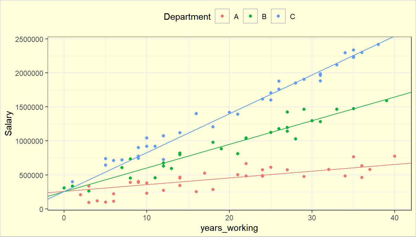
Notice that the slope is the same for both firm types (i.e. lines are parallel).
Why not fit separate regression models for the different categories?
- The model assumes constant error variance \(\sigma^2\) for each category. Different models for different categories may have different estimate of the variance (i.e. \(MSE\))
- The model also assumes equal slopes. The common slope \(\beta_1\) can best be estimated by pooling the categories.
- There will be higher sample size which means better estimates and inferences.
- It easily allows for the comparison of the groups. You can even test if there is significant difference between group, which can be quantified by the slope of the dummy variable.
Interaction Effect
So far, we only discussed a what we call the “parallel slopes model”.
A parallel slopes model is not flexible: it allows for different intercepts but forces a common slope.
Suppose we want to create models wherein we have different slope parameters for different values of a specific dummy variable.
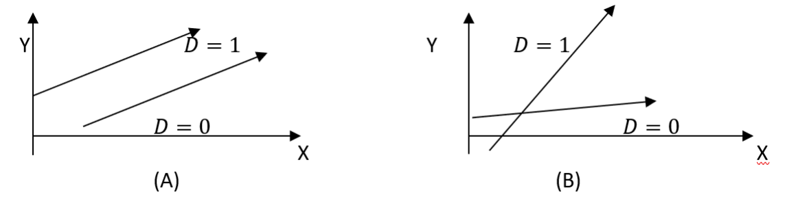
To incorporate it to our regression model, we need to multiply the dummy variable with a regressor and include the product in our model.
Model A: \(Y=\beta_0+\beta_1X+\delta D+\varepsilon\)
Intercepts: \(\beta_0, (\beta_0+\delta)\)
Slope: \(\beta_1\)
Model B: \(Y=\beta_0+\beta_1X+\delta D + \gamma X D + \varepsilon\)
Intercepts: \(\beta_0, (\beta_0+\delta)\)
Slopes: \(\beta_1, (\beta_1+\gamma)\)
Example in R
For illustration, we use the salary dataset.
| age | sex | salary |
|---|---|---|
| 21 | male | 20 |
| 57 | female | 77 |
| 32 | male | 31 |
| 25 | female | 15 |
| 54 | female | 75 |
| 44 | female | 42 |
| 63 | male | 174 |
| 31 | female | 17 |
| 42 | female | 35 |
| 26 | male | 17 |
| 38 | female | 27 |
| 64 | female | 111 |
| 48 | female | 62 |
| 34 | female | 29 |
| 30 | female | 15 |
| 55 | female | 77 |
| 50 | female | 59 |
| 27 | female | 17 |
| 31 | female | 21 |
| 52 | male | 108 |
| 60 | female | 96 |
| 40 | male | 37 |
| 53 | female | 64 |
| 39 | male | 41 |
| 52 | male | 101 |
| 55 | male | 103 |
| 33 | male | 32 |
| 22 | male | 16 |
| 38 | female | 40 |
| 39 | male | 50 |
| 51 | female | 61 |
| 27 | female | 25 |
| 23 | female | 17 |
| 42 | female | 29 |
| 44 | female | 42 |
| 50 | female | 59 |
| 39 | female | 40 |
| 57 | female | 84 |
| 56 | male | 125 |
| 46 | female | 39 |
| 53 | female | 58 |
| 22 | male | 17 |
| 49 | female | 61 |
| 29 | male | 15 |
| 21 | male | 23 |
| 57 | female | 91 |
| 54 | male | 116 |
| 37 | male | 34 |
| 65 | female | 110 |
| 50 | female | 54 |
| 37 | female | 33 |
| 24 | male | 27 |
| 48 | female | 55 |
| 41 | female | 33 |
| 49 | female | 64 |
| 44 | male | 66 |
| 42 | female | 41 |
| 53 | female | 66 |
| 55 | male | 113 |
| 36 | male | 40 |
| 61 | male | 157 |
| 23 | female | 17 |
| 53 | female | 65 |
| 31 | male | 30 |
| 60 | male | 142 |
| 41 | female | 37 |
| 34 | male | 29 |
| 51 | male | 93 |
| 20 | male | 20 |
| 63 | female | 104 |
| 33 | female | 16 |
| 48 | male | 76 |
| 50 | male | 93 |
| 47 | female | 48 |
| 33 | female | 28 |
| 50 | male | 96 |
| 45 | male | 67 |
| 54 | male | 113 |
| 61 | female | 96 |
| 36 | male | 42 |
| 44 | male | 59 |
| 42 | female | 47 |
| 25 | male | 20 |
| 63 | male | 167 |
| 45 | male | 75 |
| 25 | female | 24 |
| 29 | male | 28 |
| 65 | male | 186 |
| 54 | male | 114 |
| 24 | female | 17 |
| 44 | female | 49 |
| 56 | female | 71 |
| 40 | female | 33 |
| 28 | male | 17 |
| 41 | female | 36 |
| 57 | male | 123 |
| 57 | male | 135 |
| 63 | female | 102 |
| 41 | male | 45 |
| 41 | male | 48 |
| 33 | male | 60 |
| 37 | female | 37 |
| 29 | female | 27 |
| 38 | female | 32 |
| 35 | female | 25 |
| 37 | female | 32 |
| 20 | male | 15 |
| 34 | female | 28 |
| 38 | male | 61 |
| 21 | female | 18 |
| 25 | female | 15 |
| 29 | female | 18 |
| 29 | male | 41 |
| 33 | female | 22 |
| 25 | male | 36 |
| 24 | female | 20 |
| 24 | female | 20 |
| 35 | male | 59 |
| 39 | male | 71 |
| 26 | female | 17 |
| 29 | female | 22 |
| 29 | male | 50 |
| 37 | female | 35 |
| 25 | female | 21 |
| 24 | female | 25 |
| 35 | female | 32 |
| 27 | female | 22 |
| 25 | female | 16 |
| 22 | male | 24 |
| 24 | male | 21 |
| 24 | male | 36 |
| 30 | male | 48 |
| 34 | male | 58 |
| 24 | male | 17 |
| 31 | male | 34 |
| 29 | male | 45 |
| 40 | female | 32 |
| 33 | male | 64 |
| 33 | female | 30 |
| 39 | male | 60 |
| 33 | female | 27 |
| 38 | male | 60 |
| 20 | female | 22 |
| 23 | male | 18 |
| 20 | female | 16 |
| 22 | female | 19 |
| 22 | male | 21 |
| 22 | female | 17 |
| 28 | female | 27 |
| 24 | male | 37 |
Suppose that age and sex interact in predicting the salary, or the slopes are different.
From the plot, the slope of the salary with respect to age of male employees is steeper than the female employees. In other words, the inceremental effect of age on salary interacts with sex.
A first-order model with interaction term for our example is:
\[ Y_i=\beta_0+\beta_1 X_1 + \beta_2 X_2 + \beta_3 X_{i1}X_{i2} + \varepsilon_i \]
The meaning of the parameters are as follows:
| Intercept | Slope | |
|---|---|---|
| Female | \(\beta_0\) | \(\beta_1\) |
| Male | \(\beta_0+\beta_2\) | \(\beta_1+\beta_3\) |
Thus, \(\beta_2\) indicates how much greater (or smaller) is the \(Y\)-intercept for the class coded 1 than that for the class coded 0. \(\beta_3\) indicates how much greater (or smaller) is the slope for the class coded 1 than that coded 0.
In R, when exploring interaction terms, we just put colon : between the variables that have interaction effect.
##
## Call:
## lm(formula = salary ~ age + sex + age:sex, data = salary)
##
## Residuals:
## Min 1Q Median 3Q Max
## -31.280 -8.511 -0.446 7.730 38.237
##
## Coefficients:
## Estimate Std. Error t value Pr(>|t|)
## (Intercept) -34.2726 4.3635 -7.854 7.98e-13 ***
## age 1.9393 0.1064 18.219 < 2e-16 ***
## sexmale -24.6201 6.2706 -3.926 0.000133 ***
## age:sexmale 1.2400 0.1546 8.020 3.14e-13 ***
## ---
## Signif. codes: 0 '***' 0.001 '**' 0.01 '*' 0.05 '.' 0.1 ' ' 1
##
## Residual standard error: 11.92 on 146 degrees of freedom
## Multiple R-squared: 0.8951, Adjusted R-squared: 0.8929
## F-statistic: 415.1 on 3 and 146 DF, p-value: < 2.2e-16Visualizing…
ggplot(salary, aes(x = age, y = salary, color = sex))+
geom_point()+ theme_bw()+
geom_smooth(method = "lm", se = F)
In the dataset, not only we can see that the male employees have higher salary than female on the average, but also the salary gap increases as age increases.
What does it imply if the interaction effects are significant, but the main dummy variable is not?
The slopes of the two categories are different, but their intercepts are the same.
It is the belief of many statisticians that we do not need take away the main dummy variable in the model even if it is insignificant and the interaction effect is significant.
It is mainly because of the behavior of the coefficient of the dummy variable that it becomes ”part” of the intercept coefficient in its interpretation.
In general, you should not take away ”lower” order variables when ”higher” order variables are included in the model, unless literature and logic supports it.
Exercise 8.1 You are analyzing the relationship between house price (in thousand dollars), lot area of the house (in square foot), and location (coded as 0 for rural and 1 for urban) in a dataset of 100 houses. It is a known fact that if the lot area is 0, then the price is 0. You suspect that the effect of square footage on house price might differ between rural and urban areas.
The statistical model that may describe the relationship of price and lot area can be defined as:
\[ y_i=\beta X_i + \gamma X_iD_i +\varepsilon_i \] where
- \(y_i\) is the price of house \(i\).
- \(D_i\) is a dummy variable that takes value \(0\) if house \(i\) is in rural area, \(1\) if in urban area.
- \(\beta\) is the price per square foot in rural area.
Answer/show the following:
In the model, why is it justifiable to not include an intercept term?
Using notations in the model, what is the price per square foot in urban area?
Without using matrix notations, derive the OLS estimators of the coefficients in the full model.
8.2 Polytomous Independent Variables
What if there are more than 2 categories? How do we setup the Dummy Variables?
Suppose a variable has 4 categories. Define 4 dummy variables: \(X_1, X_2,X_3,X_4\). If there are 4 dummy variables for 4 categories, we will have the identity \(X_4=1-X_1-X_2-X_3\).
What does this imply?
From the 4 variables, only 3 are independent because \(X_4\) will be dependent on the values of the other 3 dummy variables. In the regression assumptions, all regressors should be independent from each other. Therefore, we should only use 3 dummy variables if there are 4 categories.
Remarks
In general, if there are \(m\) categories, define only \(m-1\) dummy variables to indicate membership in a category.
All that are left out are lumped together into the baseline category (all other dummy variables = 0).
Selection of the Baseline category is Arbitrary! Take note though that the baseline is the category where all other categories are compared to.
Thus, it is better if the most dominant, the least dominant, the default, or the most familiar category is chosen as the baseline.
Examples of setting dummy variables for more than 2 categories
3 categories: Disability Status = not disabled, partly disabled, fully disabled \[ \begin{align} D1&=\begin{cases} 1, & \text{if the person is disabled}\\ 0, &\text{otherwise}\end{cases} \\ D2&=\begin{cases} 1, & \text{if the person is partially disabled}\\ 0, &\text{otherwise}\end{cases} \end{align} \]
This means that if \(D1=0\) and \(D2=0\), the person is not disabled.
4 categories:
Year Level of a student = I, II, III, IV \[ D1=\begin{cases} 1, & \text{1st year}\\ 0, &\text{otherwise}\end{cases} \quad D2=\begin{cases} 1, & \text{2nd year}\\ 0, &\text{otherwise}\end{cases} \quad D3=\begin{cases} 1, & \text{3rd year}\\ 0, &\text{otherwise}\end{cases} \] This means that if \(D1=D2=D3=0\), then the year level of the student is 4th year.
Example
Suppose we want to regress the annual salary of an employee with respect to age and different departments.
There are 3 departments in a company: A, B, and C. The three-category classification can be represented in the regression equation by introducing two dummy variables \(D_1\) and \(D_2\). The regression model is then
\[ Y_i=\beta_0+\beta_1X_{i1} + \gamma_1D_{1i} +\gamma_2D_{2i} + \varepsilon \]
where \(D_{1i}=\begin{cases} 1, \text{employee } i \text{ is from department B}\\ 0, \text{otherwise}\end{cases}\), \(D_{2i}=\begin{cases} 1, \text{employee } i \text{ is from department C}\\ 0, \text{otherwise}\end{cases}\)
| Age | Department | Salary |
|---|---|---|
| 38 | C | 1204460.92 |
| 46 | B | 1180508.92 |
| 29 | C | 777106.73 |
| 47 | B | 1143911.29 |
| 49 | C | 1902898.10 |
| 55 | A | 764687.13 |
| 30 | C | 921713.04 |
| 25 | A | 101277.43 |
| 59 | B | 1591115.51 |
| 56 | A | 460089.62 |
| 29 | C | 902450.49 |
| 32 | B | 631703.95 |
| 54 | A | 486890.42 |
| 55 | C | 2334375.51 |
| 45 | A | 612248.23 |
| 23 | A | 336320.00 |
| 49 | B | 1465534.82 |
| 55 | B | 1474524.73 |
| 30 | A | 382170.64 |
| 56 | A | 636563.93 |
| 39 | B | 882012.01 |
| 21 | B | 335102.08 |
| 54 | C | 2296409.62 |
| 51 | C | 1881404.03 |
| 33 | B | 592676.04 |
| 47 | A | 573165.94 |
| 24 | A | 118265.13 |
| 37 | A | 524928.31 |
| 26 | C | 709815.92 |
| 36 | C | 1400076.61 |
| 45 | C | 1602196.73 |
| 20 | B | 309938.20 |
| 40 | C | 1419015.03 |
| 31 | B | 456906.17 |
| 50 | B | 1294530.47 |
| 42 | B | 1033898.65 |
| 34 | C | 1121838.34 |
| 46 | C | 1877019.92 |
| 34 | A | 466004.30 |
| 38 | A | 285656.79 |
| 28 | B | 733866.80 |
| 26 | A | 112581.20 |
| 51 | C | 1985142.17 |
| 44 | C | 1615519.42 |
| 56 | C | 2296767.73 |
| 41 | A | 501270.60 |
| 41 | C | 1392760.27 |
| 25 | C | 739148.20 |
| 23 | B | 261178.79 |
| 32 | C | 725438.76 |
| 29 | A | 388000.20 |
| 30 | C | 1042548.17 |
| 44 | A | 481914.88 |
| 31 | C | 920542.66 |
| 38 | B | 979934.75 |
| 53 | B | 1464490.57 |
| 42 | B | 1044196.90 |
| 23 | A | 95223.12 |
| 21 | C | 398922.95 |
| 34 | B | 818534.55 |
| 48 | B | 1030033.39 |
| 29 | C | 741456.83 |
| 32 | A | 273066.43 |
| 45 | B | 1124010.23 |
| 25 | C | 643024.36 |
| 41 | B | 810309.68 |
| 60 | A | 775000.80 |
| 34 | B | 798142.07 |
| 51 | C | 1966628.29 |
| 49 | A | 474773.38 |
| 51 | C | 1962871.05 |
| 27 | C | 719235.40 |
| 48 | C | 1847994.37 |
| 27 | B | 605715.20 |
| 47 | B | 1423232.62 |
| 44 | A | 573616.24 |
| 26 | A | 221250.84 |
| 45 | C | 1706019.45 |
| 30 | A | 229963.24 |
| 29 | A | 402156.80 |
| 46 | C | 1760612.05 |
| 57 | A | 580932.18 |
| 28 | B | 451140.30 |
| 34 | A | 345555.70 |
| 32 | B | 677117.35 |
| 58 | C | 2415942.88 |
| 51 | B | 1283166.39 |
| 47 | B | 1197548.05 |
| 52 | A | 578386.78 |
| 55 | C | 2225538.29 |
| 34 | A | 453169.98 |
| 32 | C | 1072559.40 |
| 55 | C | 2240956.18 |
| 53 | C | 2116580.01 |
| 42 | A | 667160.81 |
| 44 | A | 490047.32 |
| 36 | A | 253704.48 |
| 42 | A | 484811.94 |
| 22 | A | 206055.23 |
| 28 | A | 389616.43 |
Show more
##
## Call:
## lm(formula = Salary ~ Age + Department, data = employee)
##
## Residuals:
##     Min      1Q  Median      3Q     Max
## -547138 -124745    9666  154759  435911
##
## Coefficients:
##             Estimate Std. Error t value Pr(>|t|)
## (Intercept)  -871010      84608 -10.295  < 2e-16 ***
## Age            33540       1980  16.941  < 2e-16 ***
## DepartmentB   484539      54491   8.892 3.56e-14 ***
## DepartmentC   972408      51682  18.815  < 2e-16 ***
## ---
## Signif. codes:  0 '***' 0.001 '**' 0.01 '*' 0.05 '.' 0.1 ' ' 1
##
## Residual standard error: 216900 on 96 degrees of freedom
## Multiple R-squared:  0.8797, Adjusted R-squared:  0.8759
## F-statistic: 233.9 on 3 and 96 DF,  p-value: < 2.2e-16
In this example, Department A is the baseline category.
In this model, parameters are significant, and the \(R^2\) is also good. However, we can still improve the interpretability of the model. Some of the problems of the model:
The intercept \(\beta_0\) cannot be interpreted, since \(Age=0\) is not in the dataset.
We cannot conclude yet if salary progression is faster in Department C, and slowest in Department A.
Exercise 8.2 Explore how to improve the model in predicting salary in the company based on age and department. Make sure to do the following:
Transform
agetoyears_working. Assume that all started to work at age 20 (years_working=age-20). Use this as a predictor instead of age. Now, how do we interpret the \(\beta_0\)?Include interaction of
years_workinganddepartmentto have different slopes of salary per department.Assume that the intercept of all departments are the same. That is, the average starting salary is the same regardless of department.
Show and interpret the results of the model. What is the new \(R^2\)?
The final regression lines should look like this:
Some Notes on Models with Categorical Independent Variables
- For models with more than one qualitative independent variable, we define the appropriate number of dummy variables for each qualitative variable and include them in the model.
- Models in which all independent variables are qualitative are called analysis of variance (ANOVA) models.
- Models containing some quantitative and some qualitative independent variables, where the chief independent variables of interest are qualitative and the quantitative independent variables are introduced primarily to reduce the variance error terms, are called analysis of covariance (ANCOVA) models.
8.3 ANOVA with Categorical Predictors
We will just introduce it formally here so that you will understand the theory behind the ANOVA that you encountered in Stat 115 and Stat 125.
This section will not be included in the exam, and will be discussed more in Stat 148.
Suppose you have a numeric dependent variable \(Y\) and a categorical predictor \(X\) with \(a\) levels. For example, imagine you are studying the average tensile strength of materials produced by \(a\) different manufacturing methods. Each method \(i\) produces \(n_i\) samples, and the tensile strength for the \(j^{th}\) sample in group \(i\) is \(Y_{ij}\).
The following is an example data:
| strength | method |
|---|---|
| 188 | pure |
| 191 | pure |
| 197 | pure |
| 359 | wrought |
| 262 | wrought |
| 358 | wrought |
| 364 | wrought |
| 315 | cast |
| 307 | cast |
| 165 | cast |
| 201 | cast |
| 194 | cast |
We have the following statistics:
\(\bar{y}_{..} = 192\)
\(\bar{y}_{pure.} = 192.00\)
\(\bar{y}_{wrought.} = 335.75\)
\(\bar{y}_{cast.} = 236.40\)
Recall that we can perform an F-test here to determine if there is at least 1 group with a different mean:
##             Df Sum Sq Mean Sq F value Pr(>F)
## method       2  39579   19789   6.689 0.0166 *
## Residuals    9  26626    2958
## ---
## Signif. codes:  0 '***' 0.001 '**' 0.01 '*' 0.05 '.' 0.1 ' ' 1
How is this related with ANOVA in linear regression?
Can we express this as a linear model?
As a linear model
Based on previous discussions, we can represent the categorical predictor \(X\) using \(a-1\) dummy variables.
\[ D_i= \begin{cases} 1 & \text{if observation is in group } i\\ 0 & \text{otherwise} \end{cases} \]
Using treatment coding (\(a\) as the reference group), the linear model for predicting the tensile strength using different manufacturing methods is:
\[ Y_{ij} = \beta_0 +\beta_1D_{1,ij} + \beta_2D_{2,ij} + \cdots + \beta_{a-1}D_{a-1,ij} +\varepsilon_{ij} \]
where the average tensile strength of manufacturing method \(i\) is
\[ \mu_i = \begin{cases} \beta_0 + \beta_i, & i=1,...,a-1\\ \beta_0,& i=a \end{cases} \]
Exercise 8.3 Refer to the sample dataset containing tensile strength of different materials and the methods to manufacture the material.
If cast iron is used as the baseline group, what will be the size of the design matrix \(\textbf{X}\), and how will its elements be arranged?
Decomposition
The variation in response \(y\) is summarized by the total sum of squares:
\[ SST = \sum_{i=1}^a\sum_{j=1}^{n_i}(y_{ij}-\bar{y}_{..})^2 \]
where
\(\bar{y}_{..}\) is the grand mean of the observed values \(y_{ij}\)
\(n_i\) is the number of observed values in the \(i^{th}\) group
\(\sum_{i=1}^an_i=N\) is the total number of observations.
Like in Theorem 4.11, we can also decompose this into the \(SSR\) and \(SSE\). Here, the regression sum of squares will be the treatment sum of squares.
Derivation of \(SSTr\) and \(SSE\)
In ordinary regression, the Regression sum of squares is
\[ SSR = \sum_{i=1}^a\sum_{j=1}^{n_i}(\hat{y}_{ij}-\bar{y}_{..})^2 \]
Here in one-way ANOVA model, the fitted value of all observations in group \(i\) is the corresponding group mean
\[ \hat{y}_{ij} = \bar{y}_{i.} \]
Therefore,
\[ SSR = \sum_{i=1}^a\sum_{j=1}^{n_i}(\bar{y}_{i.}-\bar{y}_{..})^2 \]
Since each term \((\bar{y}_{i.}-\bar{y}_{..})^2\) is repeated \(n_i\) times within group \(i\), we can rewrite it as:
\[ SSR = \sum_{i=1}^an_i(\bar{y}_{i.}-\bar{y}_{..})^2 \]
which is the treatment sum of squares \(SSTr\).
Following the same concept, we have the SSE:
\[ SSE = \sum_{i=1}^a\sum_{j=1}^{n_i}(y_{ij}-\hat{y}_{ij})^2=\sum_{i=1}^a\sum_{j=1}^{n_i}(y_{ij}-\bar{y}_{i.})^2 \]
Putting this together, ANOVA yields to the identity
\[\begin{matrix} \sum_{i=1}^a\sum_{j=1}^{n_i}({y}_{ij}-\bar{y}_{..})^2 & = & \sum_{i=1}^an_i(\bar{y}_{i.}-\bar{y}_{..})^2 & + & \sum_{i=1}^a\sum_{j=1}^{n_i}(y_{ij}-\bar{y}_{i.})^2\\ SST & = & SSTr & + & SSE \end{matrix}\]8.4 Regime-Switching Models
This will not be part of your exam, but you may use this on your paper.
Rationale: Suppose we want to create a regression model wherein the slope and the intercept parameters would change at different set of values or ”Regimes” of X.
The blue dashed line is the fitted line using whole dataset. However, we can see that the relationship of \(X\) and \(Y\) changes at at some value of \(X=b\). That is, \(Y\) can be seen as a piecewise function of \(X\).
To facilitate this, we will simply use the concept of dummy variables.
Two Regimes
Regime 1: \(X\leq b\) , Regime 2: \(X>b\)
Define 1 dummy variable
\[ Y=\beta_0+\beta_1X+\delta R +\gamma XR + \varepsilon \]
where \(R=\begin{cases}1, & X \leq b\\ 0, & X>b\end{cases}\)
Three Regimes
Regime 1: \(X\leq b\) , Regime 2: \(b<X\leq c\), Regime 3: \(X>c\)
Define 2 dummy variables
\[ Y=\beta_0+\beta_1X+\delta_1 R_1 + \delta_2R_2 +\gamma_1 XR_1 +\gamma_2XR_2 + \varepsilon \]
where \(R_1=\begin{cases}1, & X \leq b\\ 0, & otherwise\end{cases}\), \(R_2=\begin{cases}1, & b<X \leq c\\ 0, & otherwise\end{cases}\)
Multiple Regimes and Connected Segments
We can restrict the segments to be connected, i.e., to fit a continuous line.
The model is given by:
\[ y =\beta_0 +\beta_1 x + \delta_1(x-k_1)R_1 + \delta_2(x-k_2)R_2 + \cdots+\delta_p(x_i-k_p)R_p + \varepsilon \]
where
\(R_j = \begin{cases} 0 & \text{ if } x < k_j\\ 1 & \text{ if } x \geq k_j \end{cases}\)
\(\beta_1\) is the slope of the first regime.
\(\beta_1 +\delta_1\) is the slope of the 2nd regime.
\(\beta_1 +\delta_1 +\delta_2\) is the slope of the 3rd regime.
\(\beta_1 + \sum_{i=1}^{j-1}\delta_i\) is the slope of the \(j^{th}\) regime.
Note that if there are \(p+1\) regimes, then define \(p\) dummy variables.
Definition 8.2 The values \(b\), \(c\), and \(k_j\) in these formulations are known as change points, switch points, kink points, or knots. These are the locations in \(X\) where the relationship between \(X\) and \(Y\) shifts.
Example: Electricity Consumption vs Temperature in the Philippines
Let
\(Y\) = electricity consumption (kWh) of a household in a day
\(X\) = average outdoor temperature (°C) for the day
In the Philippines, cooling demand drives electricity usage, especially because temperatures routinely exceed 30°C.
The relationship between temperature and consumption is not linear across all temperatures. There is a regime change once the temperature rises above 28°C, because the air-conditioner begins working much harder.
Regime 1: Comfortable Temperature (Below 28°C)
The household mostly uses electric fans and natural ventilation. Electricity consumption increases slowly as temperature rises.
Regime 2: Hot Temperature (28°C and Above)
Above 28°C, the air-conditioner turns on or shifts to a stronger cooling mode (e.g., higher compressor duty cycle). Electricity consumption increases much more steeply with temperature.
This yields to the following piecewise linear regression with a kink point at 28°C.
\[ Y = \beta_0 +\beta_1X + \beta_2(X-28)R+\varepsilon \] where \(R =\begin{cases} 1, X\geq 28 \\ 0,o.w.\end{cases}\).
We will try to fit this model to a data.
Actual Data and Visualization
| temp | consumption |
|---|---|
| 26.03 | 3.94 |
| 33.04 | 9.06 |
| 27.73 | 5.98 |
| 34.36 | 7.71 |
| 35.17 | 10.48 |
| 22.64 | 5.64 |
| 29.39 | 6.22 |
| 34.49 | 9.81 |
| 29.72 | 7.55 |
| 28.39 | 6.87 |
| 35.40 | 10.02 |
| 28.35 | 6.58 |
| 31.49 | 7.44 |
| 30.02 | 6.50 |
| 23.44 | 4.93 |
| 34.60 | 8.27 |
| 25.45 | 5.35 |
| 22.59 | 3.95 |
| 26.59 | 7.86 |
| 35.36 | 10.53 |
| 34.45 | 7.77 |
| 31.70 | 7.20 |
| 30.97 | 6.79 |
| 35.92 | 10.36 |
| 31.18 | 7.27 |
| 31.92 | 7.96 |
| 29.62 | 6.59 |
| 30.32 | 6.91 |
| 26.05 | 6.99 |
| 24.06 | 5.16 |
| 35.48 | 10.89 |
| 34.63 | 7.43 |
| 31.67 | 8.17 |
| 33.14 | 8.40 |
| 22.34 | 5.40 |
| 28.69 | 6.56 |
| 32.62 | 7.53 |
| 25.03 | 5.17 |
| 26.45 | 4.66 |
| 25.24 | 4.46 |
| 24.00 | 5.68 |
| 27.80 | 6.28 |
| 27.79 | 5.89 |
| 27.16 | 6.68 |
| 24.13 | 7.45 |
| 23.94 | 4.88 |
| 25.26 | 3.22 |
| 28.52 | 7.11 |
| 25.72 | 4.88 |
| 34.01 | 8.00 |
As the plot shows, a single straight line cannot describe the relationship between temperature and electricity consumption across all temperatures.
The relationship remains linear within each temperature range, but the change in slope requires using multiple line segments.
Fitting Procedure
##
## Call:
## lm(formula = consumption ~ temp + I((temp - 28) * (temp >= 28)),
##     data = aircon_data)
##
## Residuals:
##      Min       1Q   Median       3Q      Max
## -2.24534 -0.60609 -0.08033  0.65603  2.22252
##
## Coefficients:
##                               Estimate Std. Error t value Pr(>|t|)
## (Intercept)                    0.14812    2.44244   0.061   0.9519
## temp                           0.21050    0.09395   2.241   0.0298 *
## I((temp - 28) * (temp >= 28))  0.25151    0.13706   1.835   0.0728 .
## ---
## Signif. codes:  0 '***' 0.001 '**' 0.01 '*' 0.05 '.' 0.1 ' ' 1
##
## Residual standard error: 0.9444 on 47 degrees of freedom
## Multiple R-squared:  0.7382, Adjusted R-squared:  0.727
## F-statistic: 66.25 on 2 and 47 DF,  p-value: 2.106e-14
In this R code, I((temp-28)*(temp >=28)) corresponds to the regressor \((X-28)\cdot R\)
Interpreting the Fitted Model
The fitted model is given by
\[ \widehat{y}_i = 0.15 + 0.21 \cdot x_i + 0.25\cdot (x_i-28)\cdot R_i \]
When the temperature is not greater than 28°C, the average increase in daily consumption per temperature increase is 0.21 kWh. But if the temperature exceeds 28°C, consumption increase for an increase in °C is now \(0.25 + 0.21\) kWh, or around \(0.46\) kWh.
Note: the new y-intercept when temperature exceeds 28°C is \(0.15+0.25\cdot (-28)=-7.89\), but we do not interpret this since when \(x=0\), which is less than the switch point, we use the intercept \(0.15\)
References
- Teixeira-Pinto, J. H. &. A. (2022, August 1). 2 Piecewise regression and SPlines | Machine learning for biostatistics. https://bookdown.org/tpinto_home/Beyond-Linearity/piecewise-regression-and-splines.html