Chapter 11 Autocorrelation
Recall the linear model \(Y_i=\beta_0+\beta_1X_{1i}+\beta_1X_{2i}+\cdots+\varepsilon_i\).
It is assumed that the error term \(\varepsilon_i\) is not correlated with \(\varepsilon_j\) , \(i \neq j\).
Definition 11.1 Serial Correlation/Autocorrelation is the presence of association/relationship among adjacent observations.
11.1 Usual Causes of Autocorrelation
- Adjacent residuals tend to be similar in both temporal and spatial dimensions.
- In time series economic data, residuals tend to be positively correlated, as large positive errors are followed by other positive errors and large negative errors are followed by other negative errors.
- Seasonality in either or both the dependent and independent variables.
- Observations sampled from adjacent experimental plots are spatially correlated due to external factors
11.2 Effects of Autocorrelation
- The following theorems and methodologies discussed require the assumption that \(Var(\boldsymbol{\varepsilon}) = σ^2\textbf{I}\).
- Gauss-Markov Theorem ( \(\boldsymbol{\hat{\beta}}\) is the BLUE for \(\boldsymbol{\beta}\))
- \(\hat{\boldsymbol{\beta}}\) and \(MSE\) as the UMVUEs of the \(\boldsymbol{\beta}\) and \(\sigma^2\)
- The ANOVA F-test and the General Linear Test the t-test for significance of coefficients.
- The confidence intervals and prediction intervals
- Hence, they no longer hold or are misleading to use when we have the problem of autocorrelation. They further imply the following:
Ordinary least squares (OLS) estimators are still linear and unbiased, but are not efficient in the sense that they no longer have the minimum variance.
Estimate of \(\sigma^2\) and the standard errors of the regression coefficients may be seriously understated, giving a spurious impression of accuracy.
The confidence intervals and the various tests of significance commonly employed would no longer be strictly valid.
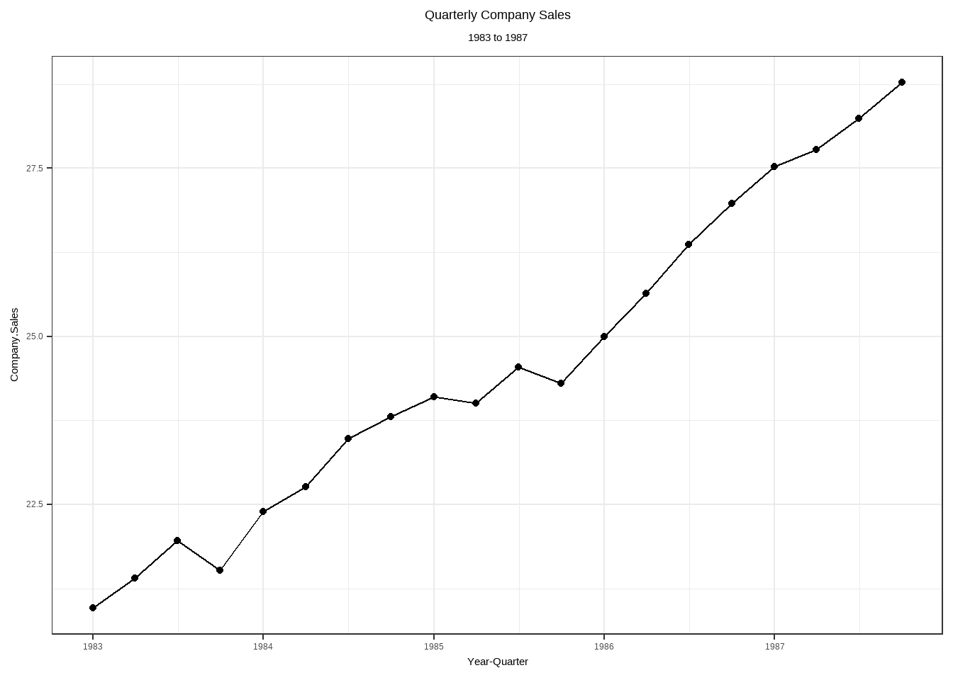
11.3 Examples of Autocorrelation
Temporal Autocorrelation
| t | Year | Quarter | Company.Sales | Industry.Sales |
|---|---|---|---|---|
| 1 | 1983 | 1 | 20.96 | 127.3 |
| 2 | 1983 | 2 | 21.40 | 130.0 |
| 3 | 1983 | 3 | 21.96 | 132.7 |
| 4 | 1983 | 4 | 21.52 | 129.4 |
| 5 | 1984 | 1 | 22.39 | 135.0 |
| 6 | 1984 | 2 | 22.76 | 137.1 |
| 7 | 1984 | 3 | 23.48 | 141.2 |
| 8 | 1984 | 4 | 23.80 | 142.8 |
| 9 | 1985 | 1 | 24.10 | 145.5 |
| 10 | 1985 | 2 | 24.01 | 145.3 |
| 11 | 1985 | 3 | 24.54 | 148.3 |
| 12 | 1985 | 4 | 24.30 | 146.4 |
| 13 | 1986 | 1 | 25.00 | 150.2 |
| 14 | 1986 | 2 | 25.64 | 153.1 |
| 15 | 1986 | 3 | 26.36 | 157.3 |
| 16 | 1986 | 4 | 26.98 | 160.7 |
| 17 | 1987 | 1 | 27.52 | 164.2 |
| 18 | 1987 | 2 | 27.78 | 165.6 |
| 19 | 1987 | 3 | 28.24 | 168.7 |
| 20 | 1987 | 4 | 28.78 | 171.7 |

Spatial Autocorrelation
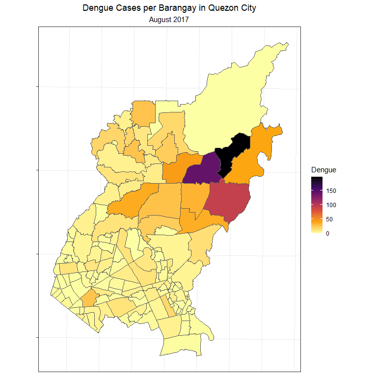
Dengue cases can be spatially clustered.
11.4 Testing for Autocorrelation
Durbin-Watson Test for Serial Autocorrelation
Recall the model: \(\textbf{Y}=\textbf{X}\boldsymbol{\beta}+\boldsymbol{\varepsilon}\), where \(\boldsymbol{\varepsilon} \overset{iid}{\sim}N(\textbf{0},\sigma^2\textbf{I})\).
For the case of autocorrelation, \(Var(\boldsymbol{\varepsilon})\neq \sigma^2\textbf{I}\).
With this, we will try to model our error term \(\varepsilon _t\) with the previous error term \(\varepsilon_{t−1}\).
One possible autocorrelation model
\[\varepsilon_t=\rho\varepsilon_{t-1}+\omega_t\]
where \(\omega_t=N(0,\sigma^2_\omega)\), \(|\rho|<1\)
Hypotheses: \(Ho:\rho=0\) vs. \(Ha: \rho \neq 0\)
The Durbin-Watson test statistic is
\[ d=\frac{\sum_{t=2}^n(e_t-e_{t-1})^2}{\sum_{t=1}^ne_t^2} \]
where \(e_t\) is the residual at time \(t\) .
Example: Recall the sales dataset and the lm object sales_model.
Exercise 11.1 Show and interpret the result of the Durbin-Watson test on the sales_model.
11.5 Remedial Measures
Re-specification
- Sometimes the best remedy is prevention. Only use cross-sectional data, instead of time-series or spatially correlated data.
- If the cause of the serial correlation is the incorrect specification, a re-specification can remedy the problem
- Use appropriate models for autocorrelated data: time-series models or spatial models
- Time Series Models will be discussed Stat 145 and Stat 192: Advance Linear Models
- Spatial Models will be discussed in Stat 197: Spatial Data Analysis
Generalized Least Squares
Similar to the problem of heteroskedasticity, this method transforms the equation with serially correlated error terms into an equation where the errors terms are no longer serially correlated (\(\delta_t\) should be IID).
Instead of using the usual linear model, we now assume that there is a dependence in the error terms.
Let our model be \[ y_t=\beta_0+\beta_1X_t+\varepsilon_t \tag{11.1} \] \[ \varepsilon_t=\rho\varepsilon_{t-1}+\delta_t \quad \text{where} \quad \delta_t \overset{iid}{\sim} N(0,\sigma^2) \]
More details about the estimation
Note that at time \(t-1\), we have \[ y_{t-1}=\beta_0+\beta_1X_{t-1}+\varepsilon_{t-1} \]
Multiply by \(\rho\), we get \[ \rho y_{t-1}=\rho \beta_0+ \rho \beta_1X_{t-1}+\rho\varepsilon_{t-1} \tag{11.2} \]
Subtract (11.2) from (11.1), we have
\[\begin{align} y_t-\rho y_{t-1} &= (\beta_0 - \rho \beta_0) + (\beta_1X_t -\rho \beta_1X_{t-1})+ (\varepsilon_t - \rho\varepsilon_{t-1})\\ y_t-\rho y_{t-1}&= \beta_0(1-\rho)+\beta_1(X_t-\rho X_{t-1}) + \delta_t\\ y_t^* &= \beta_0^* +\beta_1 X_t^* +\delta_t \tag{11.3} \end{align}\]
If \(\rho\) is known, then \(y_t^*\) and \(X_t^*\) can be computed using the data.
The reparameterized model is now free from the autocorrelation problem, therefore, the coefficients \(\beta_0^*\) and \(\beta_1\) can be estimated using OLS.
Equation (11.3) is called the Generalized Difference Equation.
However, the problem in using this equation is that \(\rho\) is unknown
The Cochrane-Orcutt Procedure
The Cochrane-Orcutt Procedure estimates \(\rho\) from the equation (11.3) above and then performs GLS.
Steps
Estimate the model \(y_t=\beta_0+\beta_1 X_t+\varepsilon_t\) without assuming autocorrelation and using OLS.
Using the residuals \(e_t\), estimate \(\rho\) using the formula
\[ \hat{\rho}=\frac{\sum_{t=2}^ne_{t-1}e_t}{\sum_{t=2}^ne_t^2} \]
Using the estimated \(\rho\), you may now compute \(y_t^*=y_t-\hat{\rho}y_{t-1}\) and \(X_t^*=X_t-\hat{\rho}X_{t-1}\).
You may now regress \(y_t^* = \beta_0^* +\beta_1 X_t^* +\delta_t\) using OLS to obtain \(\hat{\beta_0}^*\) and \(\hat{\beta_1}\). Obtain \(\hat{\beta}_0=\hat{\beta}_0^*/(1-\hat{\rho})\).
Calculate \(\hat{y}=\hat{\beta}_0+\hat{\beta}_1X_t\) and get the new residuals, \(a_t=y_t-\hat{y}_t\).
Go back to step (2), estimate a new \(\rho\) using the residuals \(a_t\).
Repeat the process until the difference between two successive estimates of \(\rho\) is small (0.01 or 0.005)
Here in Stat 136, we are only focused on linear models without autocorrelations.
Some notes for your research project:
- Use only cross-sectional data. NO NEED to perform tests for autocorrelation for this type of data.
- If you obtained a dataset with observations taken at equal time intervals (time series data), but you feel that there is no autocorrelation, only then you should use the tests for autocorrelation.
- It is not expected for you to perform GLS and the Cochrane-Orcutt procedure if autocorrelation is present. Instead,just FIND ANOTHER DATASET or topic that has no autocorrelation.