Chapter 13 On Outliers and Influential Observations
We first define the distinction between outliers and high leverage observations.
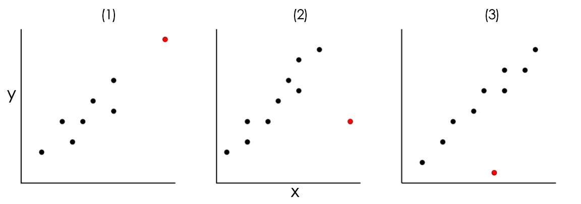
Definition 13.1 Outliers: a data point whose response \(Y\) does not follow the general trend of the rest of the data. These observations are expected to have high residuals.
Definition 13.2 High leverage points: points with extreme or unusual values of X. These are observations \(i\) with extremely high or extremely low values, or those with “unusual combination” of predictor values.
Recall that the \(i^{th}\) diagonal element of the hat matrix \(\textbf{H}\) is called the leverage of observation \(i\), where \(i=1,...,n\).
Definition 13.3 Influential Observations: its deletion singly or in combination with other observations causes substantial changes in the fitted model (including all statistics). Usually, these are observations with high leverages and high residuals, but we have to investigate further to determine whether or not they are actually influential.
Notes:
High leverage points are sometimes ”harmless” in the modelling process. We are more concerned with looking at outliers and influential observations.
Collectively, we will call these three extreme observations.
13.1 Usual Causes of Extreme Observations
There are many possible sources of extreme observations. It is important that you know the type, so you can understand how to remedy this problem.
Measurement error and Recording/encoding error
There is the inevitable occurrence of improperly recorded data, either at their source or in transcription to computer-readable form.
- Source/Measurement: Rainfall gauge malfunctioned due to typhoon, and measured 0 mm of rainfall.
- Transcription/Encoding: While inputting survey data into a spreadsheet, the encoder accidentally added an extra 0 at the end of a respondent’s salary.
Contamination
This is due to accidental inclusion of samples that do not represent the target population.
In assessment of blood sugar, some samples are accidentally mixed with glucose solution.
In assessment of heights of adults, heights of some children were accidentally included in the dataset.
Mixture of Population
This commonly occurs if you have a large population with mixed features. The subpopulations (grouping) may have influence on the variability of the variable of interest.
In analyzing test scores of students in NCR, scores of students from science highschools might show higher test scores.
In analyzing average city household income, incomes from wealthy neighborhood will appear as outliers compared to incomes from low-income neighborhood.
Part of the population (high degree of stochasticity of the population)
Some outlying data points may be legitimately occurring extreme observations. Such data often contain valuable information that improves estimation efficiency by its presence.
Only few students will get a perfect score on a hard exam.
Some trees may grow significantly taller than others.
Non-linearity or Model Misspecification
Since the data could have been generated by a model(s) other than that specified, diagnostics may reveal patterns suggestive of these alternative models.
It is important to study these extreme observations carefully and decide whether they should be retained or eliminated. You have this option for case (1) and (2).
Researchers may asses whether their influence should be reduced in the fitting process and/or the regression model revised. You may reduce influence by adding regressors for case (3) and (4).
If case (5), specify the correct model accordingly.
13.2 Implications and Effects of Extreme Observations
Why should we be concerned about it?
We want the fit to be not overwhelmingly influenced by one or few observations only.
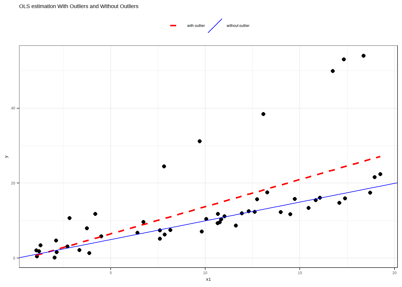
OLS is not resistant to high leverage points, outlying observations and influential observations. Large deviation from the straight line implies minimization of the sum of squares focus on that point only, allowing fewer contributions for more “normal” points.
We target for a stable set of parameter estimates. As much as possible, we want to factor out all forces that could result to undue influences to the model. “There might be other factors that can explain this unusual phenomenon”.
Extreme observations may also affect other diagnostic checking results (e.g. normality, heteroskedasticity).
13.3 Detection of High Leverage Points, Outliers, and Influential Observations
Graphical Detection
Scatter plots or residual plots can clearly reflect outlying/influential observations.
However, although much can be learned through such methods, graphical displays may not be sufficient with several variables simultaneously entering into the model.
Also, graphs may fail to show us directly what the estimated model would be if a subset of the data were modified or set aside.
Using Leverage to Detect Extreme \(X\) Values
This section explores “leverages” and how they help identify extreme values of the regressors, which can significantly impact the estimated regression function.
Recall: The estimated mean value of \(\textbf{Y}\) is
\[ \hat{\textbf{Y}}=\textbf{X}\hat{\boldsymbol{\beta}}=\textbf{X}(\textbf{X}'\textbf{X})^{-1}\textbf{X}'\textbf{Y}=\textbf{H}\textbf{Y} \]
In this definition above, \(\textbf{H}\) is the hat matrix.
If \(\textbf{H}=\{h_{ij}\}\) then the predicted value can be written as a linear combination of the other responses:
\[ \begin{align} \hat{Y}_i &=h_{i1}Y_1+h_{i2}Y_2+\cdots+h_{in}Y_n \\ &= h_{ii}Y_i+\sum_{j\neq i}h_{ij}Y_j \end{align} \]
This implies that all observations in \(Y\) also affects any predicted value of \(Y_i\)
Also, \(h_{ii}\) quantifies the influence of the observed value \(Y_i\) on the value of the predicted response \(\hat{Y}_i\)
- if \(ℎ_{𝑖𝑖}\) is small, then the observed response \(𝑦_𝑖\) plays only a small role in the value of the predicted response \(\hat{y}_i\).
- if \(h_{ii}\) is large, then the observed response \(y_i\) plays a large role in the value of the predicted response \(\hat{y}_i\). We do not want this.
Definition 13.4 (Leverage) If \(i^{th}\) diagonal element of the hat matrix \(\textbf{H}\) is given by
\[ h_{ii}=\textbf{x}_i'(\textbf{X}'\textbf{X})^{-1}\textbf{x}_i \]
where \(\textbf{x}_i\) corresponds to the vector of measurements of the \(i^{th}\) observation, then \(h_{ii}\) is the leverage (in terms of X values) of the \(i^{th}\) observation to its own fit.
Properties of Leverage
- The leverage \(h_{ii}\) is a measure of the distance between the \(x\) value for the \(i^{th}\) data point and the mean of the \(x\) values for all \(n\) datapoints.
- \(h_{ii}\) is in the range \([0,1]\) where \(1\) is high leverage, \(0\) is low leverage.
- The sum of the leverage values is equal to the number of parameters: \(tr(\textbf{H})=\sum_{i=1}^nh_{ii}=p\)
Remarks:
- The first property indicates whether or not the \(\textbf{x}_i\) values for the \(i^{th}\) observation are outlying, because \(h_{ii}\) is a measure of distance between the X values for the \(i^{th}\) observation and the means of the X values for all n observations.
- a large leverage indicates that the observation is distant from the center of the X observations.
Exercise 13.1 What is “Mahalanobis Distance” and how it is related with the leverage?
Note: This will be discussed in Stat 147.
Rule: A leverage value is usually considered to be large if it is more than twice as large as the mean leverage value; that is, leverage values greater than 2p/n are considered by this rule to indicate outlying observations with respect to the X values.
Observation \(i\) has high leverage point if \(h_{ii} > 2\frac{p}{n}\)
Example in R:
In the examples, we use the mtcars dataset.
You can use ols_leverage() from the olsrr package to show the leverage values.
##  [1] 0.14830256 0.12992351 0.06317600 0.11598460 0.17187869 0.09986745 0.14720085 0.12912656 0.45839085
## [10] 0.13597113 0.11541159 0.10343044 0.04684167 0.05527722 0.20578392 0.21066328 0.19546860 0.08593044
## [19] 0.14685385 0.14389010 0.11957800 0.11051613 0.08002229 0.10635592 0.19566514 0.09324142 0.15093650
## [28] 0.16467565 0.23978580 0.21863752 0.53168134 0.07953098- How many observations are there?
- What is the sum of the leverage values?
- From the data matrix, what is the highest leverage?
- What is the leverage threshold?
- What leverage values that exceed the cutoff value?
Detecting Outliers or Unusual \(Y\) Values
To detect outliers, a common approach is to look at observations with high residuals.
This is rather intuitive as the higher the value of the residual, the “weirder” that observation is that does not follow the linear model that we fit. Because of this, one of the most popular approach in detecting outliers is to analyze the residuals.
Definition 13.5 Standardized Residuals (internally studentized residuals)
\[ S_i=\frac{e_i}{\sqrt{MSE(1-h_{ii})}} \]
- The studentized residual follows \(T(\nu=n−p)\) based on \(n\) observations.
- Rule: outlier if \(|S_i|>t_{(\alpha/2,n-p)}\)
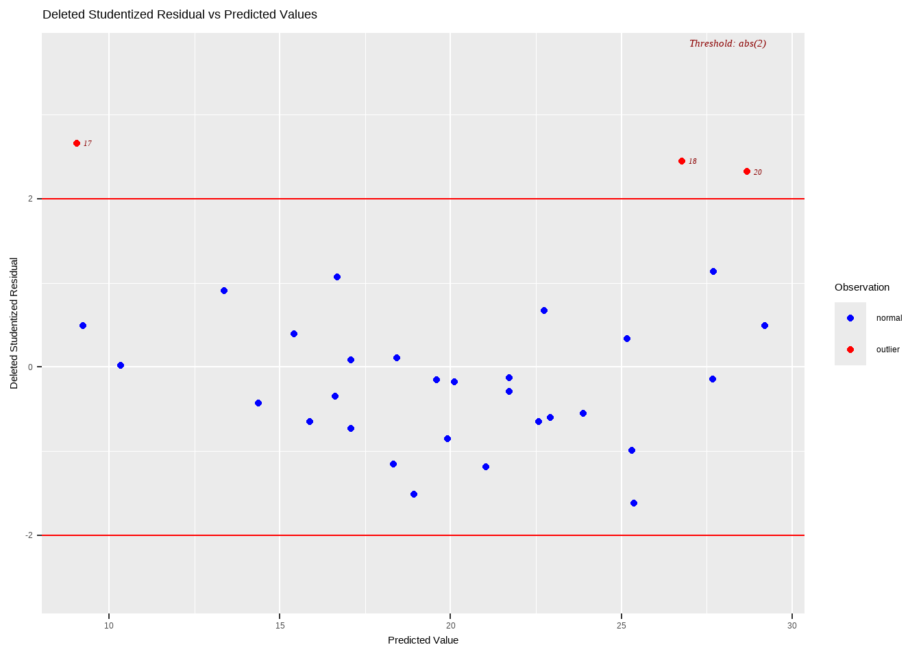
Definition 13.6 Studentized deleted residuals (externally studentized residuals)
\[ S_i^*=\frac{e_i}{\sqrt{MSE(i)(1-h_{ii})}} \]
where \(MSE(i)\) is computed from the model where \(i^{th}\) observation was deleted.
- The studentized deleted residual follows \(T(\nu=n−p-1)\) based on \(n\) observations.
- In identifying outliers using the studentized deleted residuals, we will measure the \(i^{th}\) residual \(Y_i − \hat{Y}_i\) when the fitted regression is based on the observations excluding the \(i^{th}\) observation.
- In this way, the fitted value \(\hat{Y}_i\) cannot be influenced by the \(i^{th}\) observation to be close to \(Y_i\) because this observation is not part of the data set on which the “fitted value” is based.
- Rule: outlier if \(|S_i^*|>t_{(\alpha/2,n-p-1)}\)
Common value is \(\alpha=0.05\). We can say that a specific observation is an outlier if
- \(|Si|>t_{(0.025,n−p)}\)
- \(|S_i^*|>t_{(0.025,n-p-1)}\)
For simplicity, we just use 2 as outlier treshold for all standardized/studentized residuals.
Exercise 13.2 Show that \(S_i\sim T_{(n-p)}\) and \(S^*_i\sim T_{(n-p-1)}\)
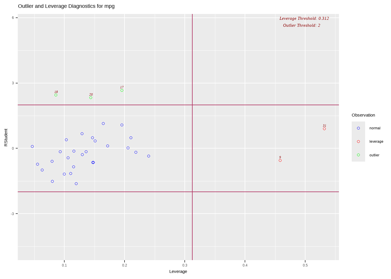
Residuals vs Leverage Plot
We can also see the high leverage points and outlying Y values in one plot.

Influential Observations Detection
After outlying observations have been identified, we then ascertain whether or not these outliers are influential in affecting the fit of the regression model, which may possibly lead to serious distortion effects
Definition 13.7 The Cook’s Distance of observation \(i\) is defined by:
\[ \begin{align} D_i&=\frac{\sum_{j=1}^n\left(\hat{Y}_j-\hat{Y}_{j(i)}\right)^2}{p\cdot MSE}\\ &=\frac{e_i^2}{p\cdot MSE}\left[\frac{h_{ii}}{(1-h_{ii})^2}\right] \end{align} \]
where \(\hat{Y}_{(i)}\) is the fitted value of \(Y\) using the model where the \(i^{th}\) observation is deleted.
an overall measure of the impact of the \(i^{th}\) observation on the estimated regression coefficients and the fitted values.
A data point having a large Cook’s D indicates that the data point strongly influences the model estimate.
There are several methods/formulas to compute the threshold used for detecting or classifying observations as outliers and we list them below
- \(4/n\)
- \(\frac{4}{n-p}\)
- \(1\)
- \(1/(n-p)\)
- \(3 \bar{D}\), where \(\bar{D}\) is the mean of the Cook’s distance values.
In this class, we use a sample size adjusted threshold given by \(\frac{4}{n-p}\)
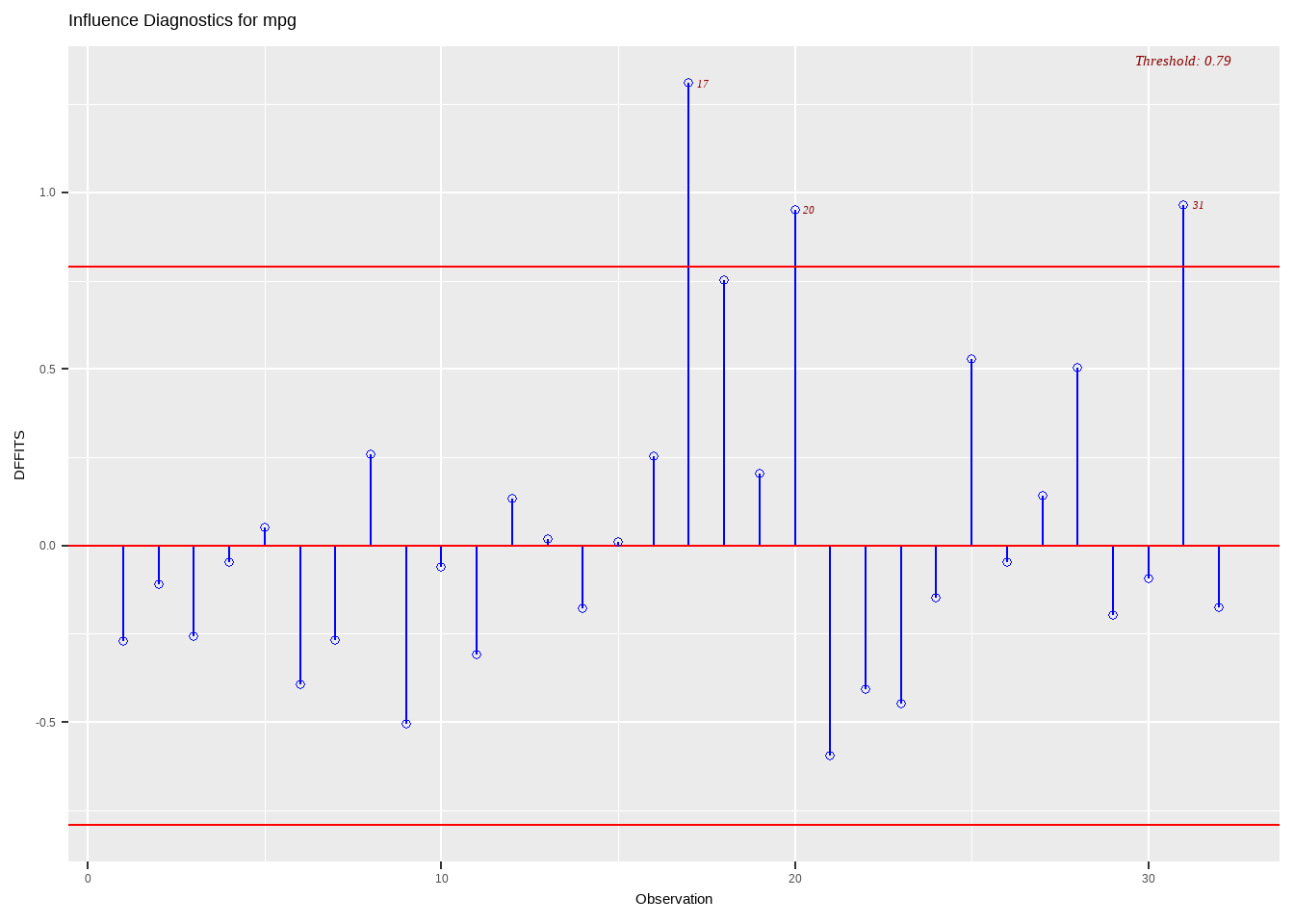
Definition 13.8 The DFFITS of an observation \(i\) is given by
\[ DFFIT_i=\left(\frac{\hat{Y}_i-\hat{Y}_{i(i)}}{\sqrt{MSE(i)h_{ii}}}\right) \]
- a scaled measure of the change in the predicted value for the ith observation and is calculated by deleting the ith observation
- a large value indicates that the observation is very influential
- General cutoff to consider is 2
- A size adjusted cutoff recommended is \(2\sqrt{p/n}\)
In this class, an observation will be considered influential if the absolute value of \(DFFITS_i\) is greater than the size-adjusted cutoff (Belsley et.al, 1980):
\[ |DFFITS_i|>2\sqrt{p/n} \]

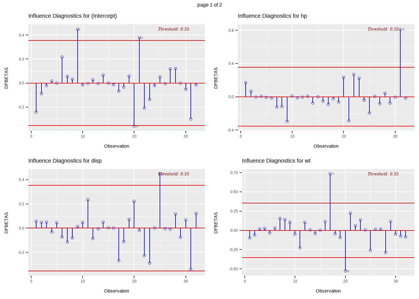
Definition 13.9 The DFBETAS of observation \(i\) on parameter \(j\) is given by
\[ DFBETAS_{ij}=\frac{\hat{\beta}_j-\hat{\beta}_j(i)}{\sqrt{MSE(i)(\textbf{X}'\textbf{X})^{-1}_{j+1}}} \]
where \((\textbf{X}'\textbf{X})^{-1}_{j+1}\) is the \((j+1)^{th}\) diagonal element of \((\textbf{X}'\textbf{X})^{-1}\)
- DFBETA measures the difference in each parameter estimate with and without the influential point
- the DFBETAS statistics are the scaled measures of the change in each parameter estimate when the \(i^{th}\) observation is deleted
- in general, a large value of DFBETA indicates that observation \(i\) is influential in estimating a given parameter\(\beta_j\)
- Rule: a general cutoff value to indicate influential observations is \(2\) and \(\frac{2}{\sqrt{n}}\) is the size-adjusted cutoff.
In this class, we say that an observation \(i\) is influential in estimating \(\beta_j\) if \(|DFBETA_{ij}|>\frac{2}{\sqrt{n}}\)

To summarize…
- High leverage point - Leverage
- Outlier Detection - Standardized and Studentized Deleted residuals
- Influential Observation Detection
- On ALL betas and fitted values - Cook’s Distance
- On a SINGLE fitted value - DFFITs
- On a SINGLE beta - DFBETAs
Exercise 13.3 The hospital.csv contains data on 112 hospitals in the United States.
Show variable details
InfctRisk: estimated percentage of patients acquiring an infection in the hospital
Stay: average length of patient stay (in days)
Age: average age of patients
Culture: average number of cultures for each patient without signs or symptoms of hospital-acquired infection, times 100
Xray: number of X-ray procedures divided by number of patients without signs or symptoms of pneumonia, times 100
Beds: number of beds in the hospital
MedSchool: does the hospital have an affiliated medical school?
Region: geographic region (NorthEast,NorthCentral, South, West)
Census: average daily census of number of patients in the hospital
Nurses: average number of full-time equivalent registed and licensed nurses
Facilities: percent of 35 specific facilities and services which are provided by the hospital
For the exercise, analyze the outliers when the following model is fitted to the dataset: \[ InfctRisk=\beta_0+\beta_1Stay+\beta_2Culture+\beta_3Xray+\varepsilon \]
Show the following plots:
Studentized Residual vs Leverage Plot
Cook’s D Chart
DFFITS plot
DFBETAs panel plots
Answer the following questions:
How many high leverage points are there?
How many outliers are there?
What are the datapoints that have overall influence to the model?
What are the datapoints that are influential to the fitted values?
What are the datapoints that are influential to each parameter estimates?
13.4 Remedial Measures
What to do with extreme observations?
They should not routinely be deleted or down-weighed because they are not necessarily bad. If they are corrected, they are the most informative points in the data.
What if an outlier/influential observation is correctly identified?
Do not drop it without any justification.
Ask yourself: Why are they outlying or influential?
Common Corrective Measures
The following are common corrective measures based on type of Outlier/Extreme Observation.
Measurement error, Recording/encoding error, or Contamination
Correct the data point.
If true data cannot be obtained (worst case scenario), you may delete the erroneous data point.
Mixture of Population, or Extreme observation is part of the population (high degree of stochasticity of the population)
Delete or Downweight (with proper justification)
Re-design the experiment or survey
Collect more data. It may be an outlier due to sampling (low probability of being part in the sample).
(for outlying Y) Add a regressor or indicator that explains the high value of Y.
Non-linearity or Model Misspecification
Transform
Consider a different model
Disclaimer: If a remedial measure is listed under a type of extreme observation problem, it does not necessarily mean that it is exclusively used for that problem. Also, the above list is nonexhaustive.
Procedure for f Outliers
The goal of this procedure is to determine if an outlier is due to chance or due to other explanations.
This involves forming prediction intervals, and determining if the outlying \(Y_0\) still falls within the interval.
- Suppose you determined \(f\) outlying observations. Check if these are due to errors in measurement, recording, computation, or some other explainable cause.
- If they are, you can drop these outliers; postulated model should still apply to the population as a whole.
- If they are not due to measurement error, fit a new regression line to the other \((n-f)\) observations (exclude the \(f\) outliers). The outliers that are not used in fitting the new regression line can now be regarded as new observations \(Y_0, \textbf{x}_0\).
- For each outlier, obtain a \((1-\alpha)100\%\) prediction interval for \(Y_{new}\) given the observations \(\textbf{x}_0\) using the fitted model without the outliers.
- If \(Y_0\) falls within the prediction interval, the outlier is due to chance and the postulated model is still viable. It is your discretion if the outlier should be retained or not.
- If \(Y_0\) does not fall in the interval, some suitable restatement of the model is required. This means that \(Y_0\) is not due to chance, but due to some explanatory variable. DO NOT DROP THE OUTLIER IN YOUR MODEL.
(Optional Exercise)
Recall the diagnostics that you performed in the hospital dataset.
Remove all influencing observations based on Cook’s D.
Fit a new regression model using the remaining observations and same independent variables.
Create 95% prediction intervals for each of those removed observations.
Are the removed influential observations inside the prediction intervals?
Final Notes:
An outlying influential observation may be discarded or deleted from the set of observations if the circumstances surrounding the data provide explanation of the unusual observation that indicates an exceptional situation not to be covered by the model.
- Measurement error, Recording Error, Contamination
If the outlying influential observation is accurate, it may not represent an unlikely event but rather a failure of the model. Often, identification of outlying influential observations leads to valuable insights for strengthening the model.
To dampen the influence of an influential observation, a different method of estimation may be used (e.g., method of least absolute deviation).
References
- Hebbali, A. (2017). olsrr: Tools for Building OLS Regression Models [Dataset]. https://doi.org/10.32614/cran.package.olsrr