CHAPTER 6 Inference on the Slope and Mean Response, and Prediction of New Observations
Estimates of regression coefficients and fitted values are all subject to uncertainty, and assessing the amount of uncertainty is an important part of most analyses. Confidence intervals result in interval estimates, while tests provide methodology for making decisions concerning the value of a parameter or fitted value.
Aside from point estimation of parameters and the ANOVA for regression relation, we extend our inference to confidence interval and hypothesis testing of each parameter.
We also infer about the mean response of \(Y\) given values of the regressors (i.e. estimate \(E(Y|X)\) using \(\widehat{E(Y|X)}\)).
Prediction of new responses is also discussed, which is one of the main goals of regression after building the model.
6.1 Inference about the Slope Parameters
Confidence Interval Estimation for Slope Parameters
Confidence interval estimates of the parameters give a better picture than point estimates (e.g. BLUE, UMVUE). The width of these confidence intervals is a measure of the overall quality of the regression line.
A possible pivotal quantity we can use to create confidence intervals for the \(\beta_j\)s are given by the following:
\[ \frac{\hat{\beta_j}-\beta_j}{\widehat{s.e.(\hat{\beta_j})}}=\frac{\hat{\beta_j}-\beta_j}{\sqrt{MSE\underline{e}_{j+1}'(\textbf{X}'\textbf{X})^{−1}\underline{e}_{j+1}}}\sim t_{(n-p)} \] Recall Section 4.8 for the form of \(\widehat{s.e(\hat{\beta}_j)}\)
Theorem 6.1 A \((1-\alpha)100\%\) CI for \(\beta_j\) is given by \[ \left( \hat{\beta}_j \mp t_{(\frac{\alpha}{2},n-p)}\widehat{s.e.(\hat{\beta_j})} \right) \]
Notes:
- These confidence intervals have the usual frequentist interpretation.
- That is, if we are to take repeated samples of the same size at the same levels of the independent variables, and construct \((1 − \alpha)100\%\) confidence intervals for \(\beta_j\) for each sample, then approximately \((1 − \alpha)100\%\) of these intervals will contain the true value of \(\beta_j\).
- In simple linear regression, a \((1-\alpha)100\%\) CI for \(\beta_1\) is given by \[ \hat{\beta}_1\mp t_{\alpha/2,n-2}\sqrt{\frac{MSE}{\sum(x_i-\bar{x})^2}} \]
Ilustration in R
Let’s use again the Anscombe dataset with the following variables:
- \(y\):
income - \(x_1\):
education - \(x_2\):
young - \(x_3\):
urban
library(carData)
data(Anscombe)
mod_anscombe <- lm(income~education + young + urban, data = Anscombe)
In R, the confidence intervals of the regression parameters are not displayed together with the other metrics.
##
## Call:
## lm(formula = income ~ education + young + urban, data = Anscombe)
##
## Residuals:
##     Min      1Q  Median      3Q     Max
## -438.54 -145.21  -41.65  119.20  739.69
##
## Coefficients:
##              Estimate Std. Error t value Pr(>|t|)
## (Intercept) 3011.4633   609.4769   4.941 1.03e-05 ***
## education      7.6313     0.8798   8.674 2.56e-11 ***
## young         -6.8544     1.6617  -4.125  0.00015 ***
## urban          1.7692     0.2591   6.828 1.49e-08 ***
## ---
## Signif. codes:  0 '***' 0.001 '**' 0.01 '*' 0.05 '.' 0.1 ' ' 1
##
## Residual standard error: 259.7 on 47 degrees of freedom
## Multiple R-squared:  0.7979, Adjusted R-squared:  0.785
## F-statistic: 61.86 on 3 and 47 DF,  p-value: 2.384e-16
The confint() computes confidence intervals for one or more parameters in a fitted model. The 95% confidence intervals are shown by default.
##                   2.5 %      97.5 %
## (Intercept) 1785.353882 4237.572728
## education      5.861365    9.401299
## young        -10.197214   -3.511526
## urban          1.247888    2.290464
Exercise 6.1 All else being equal, which of the following increases the width of the confidence interval for the slope?
A. Increasing sample size
B. Decreasing residual variance
C. Decreasing confidence level
D. Decreasing the variability in the X-values
Hypothesis Testing for Individual Slope Parameters
Testing the parameters with p-value outputs may provide us faster interpretations compared to confidence intervals.
Recall that the statistic \(\frac{\hat{\beta_j}-\beta_j}{\widehat{s.e.(\hat{\beta_j})}}\) follows the T distribution.
Definition 6.1 (T-test for a Regression Slope) For testing \(Ho:\beta_j=0\) vs \(Ha: \beta_j\neq0\), the test statistic is \[ T=\frac{\hat{\beta_j}}{\widehat{s.e.(\hat{\beta_j})}}\sim t_{(n-p)}, \quad \text{under } Ho \] The critical region of the test is \(|T|>t_{\alpha/2,(n-p)}\)
This is somehow similar with the Section Testing that one slope parameter is 0. But instead of T-tests, F-tests are used in the next chapter.
Illustration in R
Results of the hypothesis test on individual coefficients is pretty straightforward in R. Just use the summary() function on an lm object, then the estimated coefficient, standard error, t statistic, and p-values are already summarized.
##
## Call:
## lm(formula = income ~ education + young + urban, data = Anscombe)
##
## Residuals:
##     Min      1Q  Median      3Q     Max
## -438.54 -145.21  -41.65  119.20  739.69
##
## Coefficients:
##              Estimate Std. Error t value Pr(>|t|)
## (Intercept) 3011.4633   609.4769   4.941 1.03e-05 ***
## education      7.6313     0.8798   8.674 2.56e-11 ***
## young         -6.8544     1.6617  -4.125  0.00015 ***
## urban          1.7692     0.2591   6.828 1.49e-08 ***
## ---
## Signif. codes:  0 '***' 0.001 '**' 0.01 '*' 0.05 '.' 0.1 ' ' 1
##
## Residual standard error: 259.7 on 47 degrees of freedom
## Multiple R-squared:  0.7979, Adjusted R-squared:  0.785
## F-statistic: 61.86 on 3 and 47 DF,  p-value: 2.384e-16
If the model is \(y=\beta_0+\beta_1x_1+\beta_2x_2+\beta_3x_3+\varepsilon\), after performing the 3 t-tests for \(j=1,2,3\), what are the 3 conclusions at 0.05 level of significance?
Again, the t-test presented here are for individual slope parameters. Although similar in nature and goal, hypothesis tests in the next chapter will be used to show if one model is indeed better than the other.
6.2 Inference about the Mean Response
One of the major goals usually is to estimate the mean for one or more probability distributions of \(Y\).
For given values of the independent variables, say \(\textbf{x}_h\), the expected or mean response is \(E(Y_h) =E(Y|\textbf{x}_h)= \textbf{x}'_h\boldsymbol{\beta}\).
In this section, we want to make inferences about the mean \(E(Y_h)\) for given values of the independent variable.
Point Estimation for the Mean Response
Definition 6.2 (Estimated Mean Response)
The estimated mean response corresponding to \(\textbf{x}_h\), denoted by \(\widehat{Y}_h\), is \[
\widehat{Y}_h=\textbf{x}'_h\hat{\boldsymbol{\beta}}
\]
Note: Not to be confused with the Fitted Values in Definition 4.1. Here, instead of using the same set of \(\textbf{x}\) that was used in fitting, we can now use new values of the independent variables \(\textbf{x}_h\) to estimate the expected response \(Y_h\).
This answers the question:
“What is the average value of \(Y\) when \(\textbf{x}_i=\textbf{x}_h\)?”
Theorem 6.2 The estimated mean response \(\hat{Y}_h = \textbf{x}^′_h \boldsymbol{\hat{\beta}}\) is the BLUE for \(E (Y_h)\).
Exercise 6.2 Prove Theorem 6.2
Hint
Recall result and remarks from the Gauss-Markov Theorem.
Show first that for any vector of constants \(\boldsymbol{\lambda}\) and other linear unbiased estimator \(\overset{\sim}{\boldsymbol{\beta}}\), \(Var(\boldsymbol{\lambda}'\overset{\sim}{\boldsymbol{\beta}})\geq Var(\boldsymbol{\lambda}'\hat{\boldsymbol{\beta}})\).
(This implies that a linear combination of the OLS estimators \(\hat{\beta_0},\hat{\beta_k},...,\hat{\beta_k}\) are the Best Linear Unbiased Estimators for the same linear combination of \(\beta_0,\beta_1,...,\beta_k\) )
Change notations to match the notations in Theorem 6.2
Confidence Interval for the Mean Response
For the normal error regression model, \[ \widehat{Y}_h = \textbf{x}^′_h \boldsymbol{\hat{\beta}}\sim Normal(\textbf{x}^′_h \boldsymbol{\beta}, \sigma^2\textbf{x}^′_h(\textbf{X}'\textbf{X})^{-1}\textbf{x}_h) \]Based on this distribution, a possible pivot to create a CI estimator for \(E(Y_h)\) is given by: \[ \frac{\hat{Y}_h-\textbf{x}^′_h \boldsymbol{\beta}} {\sqrt{MSE\cdot\textbf{x}^′_h(\textbf{X}'\textbf{X})^{-1}\textbf{x}_h}} \sim t_{(n-p)} \]
Theorem 6.3 A \((1-\alpha)100\%\) confidence interval for \(E(Y|\textbf{x}_h)\) \[ \left(\hat{Y}_h \mp t_{\frac{\alpha}{2}, n-p} \cdot \sqrt{MSE \cdot \textbf{x}'_h(\textbf{X}'\textbf{X})^{-1}\textbf{x}_h} \right) \]
Exercise 6.3 Based on the theorem above, show that for simple linear regression, a \((1-\alpha)100\%\) confidence interval for \(E(Y_h)\) is given by:
\[ \left(\hat{Y}_h \mp t_{\frac{\alpha}{2}, n-p}\cdot \sqrt{MSE \cdot \left(\frac{1}{n}+\frac{(x_h-\bar{x})^2}{\sum_{i=1}^n(x_i-\bar{x})^2}\right)} \right) \]
Visualization for Simple Linear Regression
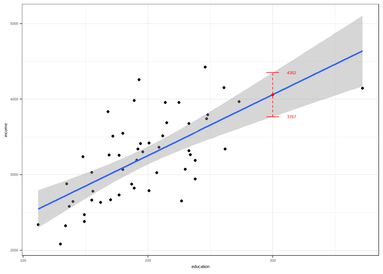
The geom_smooth layer of a ggplot object shows fitted least squares line (specified by parameter method = "lm") and the confidence bands as well (se=TRUE). Default confidence level is level=0.95.
library(ggplot2)
library(carData)
ggplot(data = Anscombe, aes(x=education, y = income))+
    geom_point()+
    geom_smooth(method = "lm", se =TRUE) +
    theme_bw()
For the CI values around an estimate \(\hat{Y}_h\) for a given value \(x_h=300\), we can use the predict function.
mod1 <- lm(income~ education, data = Anscombe)
predict(mod1, data.frame(education = 300), interval = "confidence")
## fit lwr upr
## 1 4059.75 3767.465 4352.035As you can see in the plot below, a confidence interval estimate for \(E(Y|X=300)\) is \((3767,4352)\).
Exercise 6.4 Suppose a simple linear regression model is fitted:
\[ \hat{y}=\hat{\beta}_0+\hat{\beta}_1x \]
You are given the following:
\(\hat{\beta}_0=2.5\), \(\hat{\beta}_1=1.8\)
\(n=25\), \(\bar{x}=10\)
\(s^2_x=8, s^2_y=4\)
\(MSR = 8\)
Find a 95% confidence interval for the mean response at \(x_h=12\).
Hypothesis Testing for the Mean Response
Following previous results, we have the following test about the expected or mean response.
Theorem 6.4 The following can be used to test the following hypotheses:
\[ Ho:E(Y_h)=d\quad\text{vs}\quad Ha:E(Y_h) \neq d \]
Test Statistic: \[ t=\frac{\hat{Y}_h-d} {\sqrt{MSE\cdot\textbf{x}^′_h(\textbf{X}'\textbf{X})^{-1}\textbf{x}_h}} \]
Critical Region: Reject \(Ho\) if \[ t>t(\alpha/2,n-p) \]
6.3 Prediction of a new observation
In the case that we are not estimating a parameter but predicting a particular value of the random variable \(Y_i\) for a particular \(\textbf{x}_i\) , we can use the concept of prediction intervals. In this case, we are predicting an individual outcome drawn from the distribution of \(Y\).
“What value of \(Y\) might we observe for a new case with \(\textbf{x}_i=\textbf{x}_h\)?”
The goal is not just to estimate the conditional mean \(\mathbb{E}[Y_h|\textbf{x}_h]\), but to predict the new value of a new observation:
\[ Y_{h(new)}=\textbf{x}_h'\boldsymbol{\beta}+\varepsilon_h \]
The new observation on \(Y\) is viewed as the result of a new trial, independent of the trials on which the regression analysis is based. We also assume that the underlying regression model applicable for the basic sample data continues to be appropriate for the new observation \(Y_{h(new)}\).
Definition 6.3 (Predicting a new observation and the Prediction Error)
We predict a new observation \(Y_{h(new)}\) using \(\widehat{Y}_{h(new)}=\textbf{x}_h'\hat{\boldsymbol{\beta}}\)
The prediction error is \(Y_{h(new)}-\hat{Y}_{h(new)}\)
Remarks
The new observation \(Y_{h(new)}\) is a random variable.
\(Y_{h(new)}\sim N(\textbf{x}_h'\boldsymbol{\beta},\sigma^2)\)
The value of \(Y_{h(new)}\) cannot be observed, only predicted.
For this case, the predicted value is just the estimated mean
Theorem 6.5 The variance of the prediction error is
\[ Var(Y_{h(new)}-\hat{Y}_{h(new)})=\sigma^2(1+\textbf{x}'_h(\textbf{X}'\textbf{X})^{-1}\textbf{x}_h) \]
Prediction Intervals
Case 1: All parameters are known
If all parameters are known, take note that \[ Y_i\sim N(\textbf{x}_i'\boldsymbol{\beta},\sigma^2) \] A possible pivot to create a prediction interval is: \[ \frac{Y_i-\textbf{x}_i'\boldsymbol{\beta}}{\sigma}\sim N(0,1) \] From this, we can now have the following prediction interval for a new observation \(Y_{h(new)}\):
Theorem 6.6 A prediction interval for \(Y_{h(new)}\) is given by \[ (\textbf{x}_h'\boldsymbol{\beta} \mp z_{\alpha/2}\sigma) \]
Case 2: All parameters are unknown
Assumptions:
parameters \(\boldsymbol{\beta}\) and \(\sigma^2\) have already been estimated (but true value still unknown)
the given \(\textbf{x}_h\) must be independent of the previous sample
Theorem 6.7 A prediction interval for \(Y_{h(new)}\) is given by: \[ (\textbf{x}_h'\hat{\boldsymbol{\beta}} \mp t_{(\alpha/2,n-p)}\sqrt{MSE\cdot[\textbf{x}^′_h(\textbf{X}'\textbf{X})^{-1}\textbf{x}_h+1]}) \]
Remarks:
- Why is there a “+1” in Case 2?
- Note that in predicting a new observation, you are estimating two things technically:
- The mean response \(E(Y_h)\)
- The new observation based on the estimated mean response.
- Let us define the prediction error as \(Y_h-\hat{Y}_h\). The variance of the prediction error is \(Var(Y_h-\hat{Y}_h)= Var(\varepsilon_h)+Var(\hat{Y}_h)\). This implies that there are two sources of variability:
- The random error \(\varepsilon_h\) that generates the point \(Y_h\).
- The uncertainty in the estimated regression line
- For the case of unknown parameters, prediction intervals are wider than confidence intervals.
- Note that in predicting a new observation, you are estimating two things technically:
- How to interpret prediction intervals?
- Under the assumption that the additional observation is obtained in the same way as you obtained your past data, we can interpret \((1 − \alpha)\) as the probability that the new observation is inside the prediction interval.
- This makes sense since we assume that the \(Y_{h(new)}\) is a random variable. Contrary to Confidence Intervals where the constructed interval is for a fixed parameter value that is not random.
- Take note again of the caution of using the model for \(\textbf{x}_h\) not being inside the ”scope” of the model!
Illustration of Predicting a Response in R
Recall the Anscombe dataset.
We use education, young, and urban as linear predictors of income.
library(carData)
data(Anscombe)
mod <- lm(income ~ education + urban + young, data = Anscombe)
summary(mod)
##
## Call:
## lm(formula = income ~ education + urban + young, data = Anscombe)
##
## Residuals:
## Min 1Q Median 3Q Max
## -438.54 -145.21 -41.65 119.20 739.69
##
## Coefficients:
## Estimate Std. Error t value Pr(>|t|)
## (Intercept) 3011.4633 609.4769 4.941 1.03e-05 ***
## education 7.6313 0.8798 8.674 2.56e-11 ***
## urban 1.7692 0.2591 6.828 1.49e-08 ***
## young -6.8544 1.6617 -4.125 0.00015 ***
## ---
## Signif. codes: 0 '***' 0.001 '**' 0.01 '*' 0.05 '.' 0.1 ' ' 1
##
## Residual standard error: 259.7 on 47 degrees of freedom
## Multiple R-squared: 0.7979, Adjusted R-squared: 0.785
## F-statistic: 61.86 on 3 and 47 DF, p-value: 2.384e-16Now, suppose we want to predict the income of 2 new states, and data for education, young ratio, and urban ratio are available. Data is stored in dataframe new_states.
new_state1 <- c(education = 190, young = 350, urban = 500)
new_state2 <- c(education = 300, young = 275, urban = 250)
new_states <- data.frame(rbind(new_state1, new_state2))
new_states
## education young urban
## new_state1 190 350 500
## new_state2 300 275 250Note that the new dataframe new_states has the same columns required for the predictors stored in the lm object mod.
We can estimate the expected income , which is the same as predicting the income, of the two new states given the predictors using the fitted model mod and the function predict(). Confidence interval or prediction interval can be shown by using the interval= argument.
# estimate of expected income with 95% confidence intervals
predict(mod, new_states, interval = "confidence", level = 0.95)
## fit lwr upr
## new_state1 2946.975 2828.350 3065.600
## new_state2 3858.205 3351.406 4365.004# prediction of income with 95% prediction intervals
predict(mod, new_states, interval = "prediction", level = 0.95)## fit lwr upr
## new_state1 2946.975 2411.320 3482.63
## new_state2 3858.205 3130.401 4586.01Notice that the confidence interval of \(E(Y_{h(new)})\) is narrower than the prediction interval of \(Y_{h(new)}\)
Exercise 6.5 In terms of interpretation, what is the difference between the Expected Value and the Predicted Value in regression?
Exercise 6.6 In a regression model predicting income from years of education, you compute the following at \(x_h=12 \text{ years}\):
- 95% CI for the mean response: (30,000, 32,000)
- 95% prediction interval for a new observation: (26,000, 36,000)
Question: why is the prediction interval wider than the confidence interval?
- The prediction interval uses a smaller standard error.
- The confidence interval ignores the variability of the mean.
- The prediction interval includes both model error and individual variability.
- The prediction interval is always 10,000 units wider by definition.
6.4 Assessment of Predictive Ability of Model
Selecting a model based on metrics that are calculated using observations not included in the estimation helps prevent overfitting.
Cross Validation using Train and Test Sets
In this section, we perform a cross validation method to assess how good the model is in predicting a set of new observations. Often, we first split the dataset into a training set and a test set.
Definition 6.4 (Train and Test Sets)
- Train dataset is a subset of the original dataset that we use to create the model.
- Test dataset is a subset of the original dataset that we assume to be new or unobserved, which we use to predict values of the dependent variable to assess the model.
Remarks:
- It is common to split the dataframe to 70-30. 70% of the dataset will be used for training the model, and the rest will be used for testing the model.
- In linear regression, observations belonging in the train or test set are chosen randomly (SRS).
- Prior to splitting, we already assumed that observations in the dataset were sampled independently. Even if we take a sample without replacement (SRSWOR) from the already collected dataset, independence assumption will not be violated if we regress using the training set.
Illustration in R:
Choosing observations randomly that will belong in the train and test datasets.
# obtaining random numbers, 70% of the number of observations
index <- sample(1:nrow(Anscombe),
        size = round(nrow(Anscombe)*0.7,0))
index
## [1] 25 10 15 32 18 45 28 39 5 21 36 17 2 8 7 42 22 16 12 43 9 33 31 3 24
## [26] 46 19 44 49 23 14 1 40 27 50 29# splitting the dataset using the random numbers generated
library(carData)
train <- Anscombe[index,]
test <- Anscombe[-index,]Test dataset:
| education | income | young | urban | |
|---|---|---|---|---|
| MA | 168 | 3835 | 335.3 | 846 |
| CT | 193 | 4256 | 341.0 | 774 |
| IN | 194 | 3412 | 359.3 | 649 |
| MI | 233 | 3675 | 369.2 | 738 |
| NE | 148 | 3239 | 349.9 | 615 |
| WV | 149 | 2470 | 328.8 | 390 |
| FL | 191 | 3191 | 336.0 | 805 |
| MS | 130 | 2081 | 385.2 | 445 |
| AR | 134 | 2322 | 351.9 | 500 |
| OK | 135 | 2880 | 329.8 | 680 |
| TX | 155 | 3029 | 369.4 | 797 |
| WY | 238 | 3190 | 365.6 | 605 |
| WA | 215 | 3688 | 341.3 | 726 |
| OR | 233 | 3317 | 332.7 | 671 |
| HI | 212 | 3513 | 382.9 | 831 |
Train dataset:
| education | income | young | urban | |
|---|---|---|---|---|
| VA | 180 | 3068 | 353.0 | 631 |
| OH | 172 | 3509 | 354.5 | 753 |
| MN | 262 | 3341 | 365.4 | 664 |
| TN | 137 | 2579 | 342.8 | 588 |
| ND | 177 | 2730 | 369.1 | 443 |
| UT | 201 | 2790 | 412.4 | 804 |
| SC | 149 | 2380 | 376.7 | 476 |
| MT | 238 | 2942 | 368.9 | 534 |
| RI | 180 | 3549 | 327.1 | 871 |
| KA | 196 | 3303 | 339.9 | 661 |
| LA | 162 | 2634 | 389.6 | 661 |
| MO | 177 | 3257 | 336.1 | 701 |
| NH | 169 | 3259 | 345.9 | 564 |
| NJ | 214 | 3954 | 333.5 | 889 |
| NY | 261 | 4151 | 326.2 | 856 |
| CO | 192 | 3340 | 358.1 | 785 |
| DE | 248 | 3795 | 375.9 | 722 |
| IO | 234 | 3265 | 343.8 | 572 |
| IL | 189 | 3981 | 348.9 | 830 |
| NM | 227 | 2651 | 421.5 | 698 |
| PA | 201 | 3419 | 326.2 | 715 |
| AL | 112 | 2337 | 362.2 | 584 |
| KY | 140 | 2645 | 349.3 | 523 |
| VT | 230 | 3072 | 348.5 | 322 |
| DC | 246 | 4425 | 352.1 | 1000 |
| NV | 225 | 3957 | 385.1 | 809 |
| SD | 187 | 2876 | 368.7 | 446 |
| AZ | 207 | 3027 | 387.5 | 796 |
| CA | 273 | 3968 | 348.4 | 909 |
| MD | 247 | 3742 | 364.1 | 766 |
| WI | 209 | 3363 | 360.7 | 659 |
| ME | 189 | 2824 | 350.7 | 508 |
| ID | 170 | 2668 | 367.7 | 541 |
| NC | 155 | 2664 | 354.1 | 450 |
| AK | 372 | 4146 | 439.7 | 484 |
| GA | 156 | 2781 | 370.6 | 603 |
Creating a model using the training dataset.
##
## Call:
## lm(formula = income ~ education + young + urban, data = train)
##
## Residuals:
##     Min      1Q  Median      3Q     Max
## -403.04 -145.06  -21.90   85.49  503.72
##
## Coefficients:
##              Estimate Std. Error t value Pr(>|t|)
## (Intercept) 3212.8284   640.9988   5.012 1.92e-05 ***
## education      8.1169     0.9187   8.835 4.29e-10 ***
## young         -7.2888     1.7324  -4.207 0.000195 ***
## urban          1.5343     0.2710   5.661 2.90e-06 ***
## ---
## Signif. codes:  0 '***' 0.001 '**' 0.01 '*' 0.05 '.' 0.1 ' ' 1
##
## Residual standard error: 237.1 on 32 degrees of freedom
## Multiple R-squared:  0.8342, Adjusted R-squared:  0.8186
## F-statistic: 53.66 on 3 and 32 DF,  p-value: 1.385e-12
Now, using the model that we trained from the training dataset, we predict the income in the test dataset.
##       MA       CT       IN       MI       NE       WV       FL       MS
## 3430.506 3481.415 3164.364 3545.312 2807.338 2624.040 3549.188 2143.114
##       AR       OK       TX       WY       WA       OR       HI
## 2502.684 2948.051 3001.259 3408.079 3584.155 3708.559 3417.687
We now compare the predicted values and the actual values in the test dataset.
| actual.income | predicted.income | |
|---|---|---|
| MA | 3835 | 3430.506 |
| CT | 4256 | 3481.415 |
| IN | 3412 | 3164.364 |
| MI | 3675 | 3545.312 |
| NE | 3239 | 2807.338 |
| WV | 2470 | 2624.040 |
| FL | 3191 | 3549.188 |
| MS | 2081 | 2143.114 |
| AR | 2322 | 2502.684 |
| OK | 2880 | 2948.051 |
| TX | 3029 | 3001.259 |
| WY | 3190 | 3408.079 |
| WA | 3688 | 3584.155 |
| OR | 3317 | 3708.559 |
| HI | 3513 | 3417.687 |
We can visualize the relationship of the actual and predicted values using a scatterplot, with a \(y=x\) line.
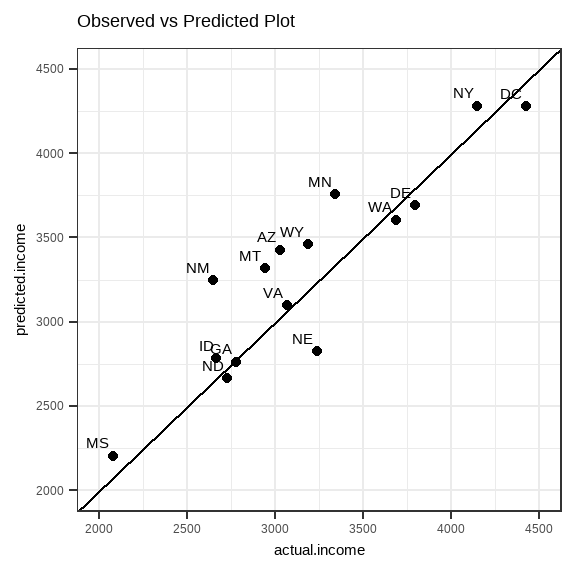
Through visual inspection, the model created using the training dataset seems to predict the income well, since the predicted values and the actual values are close to each other.
Remarks:
- After obtaining predicted values on the test dataset, we compare them against the actual values in the test dataset.
- Some metrics that can be used to compare the predicted vs actual values are the \(RMSE\), \(MAE\), \(MAPE\), among others. Computations of these metrics are available in the R package
Metrics - These metrics will not be discussed further in Stat 136, but you can explore them on your own.
Prediction Error Sum of Squares (PRESS)
Definition 6.5 (Prediction Error Sum of Squares) The PRESS statistic involves regressing using all observations but the \(i^{th}\) observation to obtain a predictor of \(Y_i\) and forming the sum of squared differences between the observed and predicted values for \(i = 1, 2, . . . , n\).
Delete first set of observations \(i\) on the independent and dependent variables.
Fit the proposed regression model to the remaining \((n − 1)\) to obtain estimates \(\hat{\boldsymbol{\beta}}_{(i)}\), the estimate for \(\boldsymbol{\beta}\) when observation \(i\) was removed in the dataset.
Use the fitted model to predict \(Y_i\) by \(\hat{Y}_{(i)}=\textbf{x}_{i}'\hat{\boldsymbol{\beta}}_{(i)}\), where \(\textbf{x}_i\) is the vector of values of independent variables for observation \(i\).
Obtain a predictive discrepancy \((Y_i − \hat{Y}_{(i)})\)
Repeat steps 1 to 4 for \(i=1,...,n\)
- Calculate the sum of squares of the predictive discrepancy\[ PRESS=\sum_{i=1}^n(Y_i-\hat{Y}_{(i)})^2 \]
Notes:
The PRESS statistic is a leave-one-out refitting and prediction method, as described in Allen (1971). This is related with the Jackknife method of model validation approach.
The PRESS statistic tells you how well the model will predict new data that is not included in creating the model.
The smaller the value of PRESS, the better.
PRESS has the advantage of providing a lot of detailed information about the stability of various fitted models over the data space.
Disadvantages
A major disadvantage is the enormous amount of computation required.
The range of values of PRESS may be dependent on the scaling and range of values of the dependent variable, which makes it hard to interpret sometimes. You need to compare this to the PRESS of other models to be interpretable.
Illustration in R
The ols_press() function in olsrr package calculates the PRESS statistic for a model, but not for all possible regression. We can just calculate them manually for candidate regression models.
## [1] 17392465## [1] 4793604## [1] 4194578Predicted \(R^2\)
PRESS can also be used to calculate the predicted \(R^2\) (denoted by \(𝑅_{pred}^2\)) which is generally more intuitive to interpret than PRESS itself.
Definition 6.6 (Predicted R-squared) The predicted \(R^2\) is defined as
\[ R^2_{pred}=1-\frac{PRESS}{SST} \]
Like the coefficient of determination, the predicted \(R^2\) also ranges from 0 to 1.
The predicted \(R^2\) is a useful way in validating predictive ability of the model without splitting the data into training and test sets.
You can use the
ols_pred_rsq()function from theolsrrpackage to compute the \(R^2_{pred}\) of a model.## [1] 0.7325135
6.5 The Inverse Prediction Problem (Optional)
Definition 6.7 A regression model of \(Y\) on \(X\) may be used to predict the value of \(X\) which gave rise to a new observation \(Y\) . This is known as an inverse prediction.
Example: A regression analysis of the amount of decrease in cholesterol level \((Y)\) achieved with a given dosage of a new drug \((X)\) has been conducted, based on observations for 50 patients. A physician is treating a new patient for whom the cholesterol level should decrease to amount \(Y_{h(new)}\). It is desired to estimate the appropriate dosage level \(X_{h(new)}\) to be administered to bring about the needed cholesterol decrease \(Y_{h(new)}\).
The model is assumed to be \(Y_i=\beta_0+\beta X_i+\varepsilon_i\) and the estimated regression line is \(\hat{Y}_i=\hat{\beta}_0+\hat{\beta}X_i\).
If a new observation \(Y_{h(new)}\) becomes available, a natural point estimator for level \(X_{h(new)}\) which gave rise to \(Y_{h(new)}\) is
\[ \hat{X}_{h(new)}=\frac{\hat{Y}_{h(new)}-\hat{\beta}_0}{\hat{\beta}} \]
Illustrations:
- Suppose \(Y\) = mortality rate of grouper juveniles and \(X\) = concentration of heavy metal (lead), and the estimated regression model is \(\hat{Y}=30+0.60X\). What should be the value of \(X\) so \(\hat{Y}=50\) is attained?
- Suppose \(Y\) = sales and \(X\) = expenditure to print advertisement. Suppose that a 10% increase in sales is targeted, current sales level is at 100 → 10% increase to 110. Can it be supported by increase in expenditure to print advertisement? Suppose \(\hat{Y} = 100 + 2.5X\) , find \(X\) when \(\hat{Y} = 110\).
Remarks:
Estimates for \(X\) are functions of parameter estimates. Standard errors for the predictions can be approximated from the standard errors of the least square estimates of the regression coefficients.
However, since the standard errors of the predictions depends on the original regression model, one may encounter problem in using them for prediction intervals. Sometimes the upper and lower bounds may create some problems.
The inverse prediction problem is also known as a calibration problem since it is applicable when inexpensive, quick, and approximate measurements \(Y\) are related to precise, often expensive, and time-consuming measurements \(X\) based on \(n\) observations.
The resulting regression model is used to estimate the precise measurement \(X\) for a new approximate measurement \(Y\). One can easily extend the notion of the calibration problem to two or more independent variables. However, calibration should be done to one independent variable only. That is, hold other independent variables constant while finding the value \(X_j\) for the \(j^{th}\) independent variable.
The inverse prediction problem has aroused controversy among statisticians. Some statisticians have suggested that inverse predictions should be made in direct fashion by regressing \(X\) on \(Y\). That is, use the \(X\) as dependent variable, and use \(Y\) as the independent variable. This regression is called inverse regression.