10 Probit Regression (Stata)
10.1 Lab Overview
This web page provides a brief overview of probit regression and a detailed explanation of how to run this type of regression in Stata. Download the script file to execute sample code for probit regression. We’ll be running the same analyses as the logistic regression lab, so you can click back and forth to see the differences between the two types of models.
Research Question: What rookie year statistics are associated with having an NBA career longer than 5 years?
Lab Files
Data:
Download nba_rookie.dta
Script File:
Download lab5_PR.do
10.2 Probit Regression Review
In probit regression you are predicting the z-score change of your outcome as a function of your independent variables. To understand why our dependent variable becomes the z-score of our outcome, let’s take a look at the binomial distribution.
Binary outcomes follow what is called the binomial distribution, whereas our outcomes in normal linear regression follow the normal distribution. In this logistic regression, we assumed that the probabilities following this binomial distribution fell on a logistic curve. In probit regression, we instead assume that the probabilities fall on a very similar curve, the cumulative normal curve. Let’s review the normal curve, the cumulative normal curve, and the difference between the logistic curve and the cumulative normal curve.
Plot 1: The Normal Distribution
You should be very familiar with the bell curve, aka the normal distribution, aka the Gaussian distribution. I’m emphasizing the word Gaussian because it’s the technical statistical name that you will see pop up in explanations of probit regression and it can be confusing if you don’t know what it is. It’s just the normal distribution, aka this:
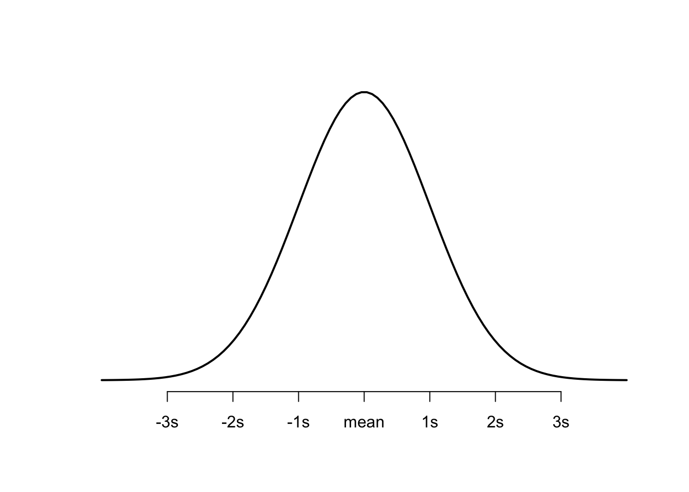
This plot shows the probability of a value falling above or below the mean at any given point.
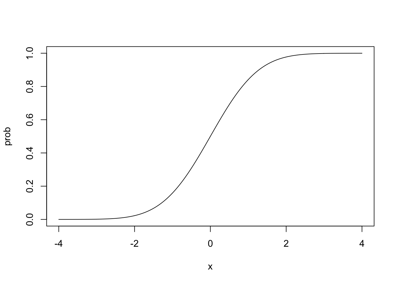
Plot2: The Cumulative Normal Distribution
This is the normal distribution curve, but cumulative. So instead of plotting the probability at a point. It plots the probability of getting that value and any value below that. It is the equation of this curve that we use to model probit regresion.
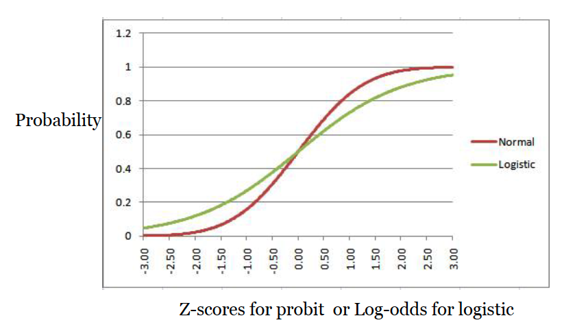
It is very very similar to the logistic curve. But it’s not as mathematically convenient as the logistic curve equation, so probit has become the less-often used curve for binary regression. As a reminder, this is what the normal cumulative curve and the logistic curve look like lined up on top of each other.
Here’s a shortened version of how we use the equation for this curve to get to our probit regression.
This equation says that the probability of our outcome being equal to one can be calculated by putting our familiar linear equation inside the equation for the cumulative normal distribution (aka the curve above). \(\Phi\) refers to the cumulative normal distribution function.
\[P(Y=1) = \Phi(\beta_0 + \beta_1X_1 + ... \beta_kX_k) \]
But how in the world are we supposed use this equation in a regression?
We want our handy linear equation to exist all on it’s own on the right hand side
(\(\beta_0 + \beta_1X_1 + ... \beta_kX_k\)) because again, we want to be able to predict our outcome by adding together the effects of all our covariates using that linear equation. We solve for that linear equation by taking the inverse of the normal distribution curve.
\[ \Phi^{-1}(P(Y = 1)) = \beta_0 + \beta_1X_1 + ... \beta_kX_k\] Now that’s more like it! On the right side of the equals sign we have our familiar linear equation. On the left side of the equals sign we have our outcome put through the inverse normal distribution function. That sounds complicated, but all it really means its our outcome is a now a z-score. You may remember from basic stats. You use a z-score table to find a probability (basic stats throwback!). You reverse that to get from a probability to a z-score.
10.2.1 Interpreting Z-Scores via Probability
A one unit change in X is associated with a one unit change
in the z-score of Y.
Running a probit regression in Stata is exactly the same as running a logistic regression. BUT your outcomes are now in z-score units rather than log-odds. But just like log-odds, z-score units are not intuitive and probably won’t mean anything to your reader. There is no equivalent of an odds ratio for probit regression, because we’re not working with odds or log-odds outcomes anymore. That means our option for interpreting probit regression results is our good buddy probability. If you’re interested in the math behind how Stata goes from z-score units to probability, brush up on your z-score table knowledge and the normal distribution functions. It’s pretty mathematically complicated to calculate probability from a normal distribution, and we have to approximate it (that’s what z-tables are for), so you’ll never need to do it by hand in probit regression. Practically, we’ll just use the margins command to translate our coefficients into predicted probabilities and marginal effects (aka changes in probability).
10.2.2 Assumptions of the model
(1) The outcome is binary
A binary variable has only two possible response categories. It is often referred to as present/not present or fail/success. Examples include: male/female, yes/no, pass/fail, drafted/not drafted, and many more!
(2) The probit (aka z-score) of the outcome and independent variable have a linear relationship
Although a smoothing line of your raw data will often reveal an s-shaped relationship between the outcome and explanatory variable, the probit of the outcome vs the explanatory variable should have a linear relationship.
How to address it?
Like a linear regression, you can play around with squared and cubed terms to see if they address the curved relationship in your data.
(3) Normally distributed errors
In logistic regression, we do not expect errors to be normally distributed. But because we are modeling probit regression based on a cumulative normal distribution, this assumption from logistic regression returns. Again if the sample size is large enough (>20 cases) violating this assumption is not too worrysome.
(4) Errors are independent
Like linear regression we don’t want to have obvious clusters in our data. Examples of clusters would be multiple observations from the same person at different times, multiple observations withing schools, people within cities, and so on.
How to address it?
If you have a variable identifying the cluster (e.g., year, school, city, person), you can run a probit regression adjusted for clustering using cluster-robust standard errors (rule of thumb is to have 50 clusters for this method). However, you may also want to consider learning about and applying a hierarchical linear model.
(5) No severe multicolinearity
This is another carryover from linear regression. Multicollineary can throw a wrench in your model when one or more independent variables are correlated to one another.
How to address it?
Run a VIF (variance inflation factor) to detect correlation between your independent variables. Consider dropping variables or combining them into one factor variable.
Differences to logistic regression assumptions
Like logistic regression, probit regression DOES NOT require an assumption of homoskedasticity, but it does assume that the errors are normally distributed, unlike logistic regression.
10.2.3 Pros and Cons of the model
Pros:
- Some statisticians like assuming the normal distribution over the logistic distribution.
Cons:
- Z-scores are not as straightforward to interpret as the outcomes of a linear probability model.
- We can’t use odds ratios to describe findings.
- It’s more mathematically complicated than logistic regression.
- Economists like that you can do more complicated analysis with probit that logit cannot handle.
10.3 Running a probit regression in Stata
Now we will walk through running and interpreting a probit regression in Stata from start to finish. Like logistic regression, the trickiest piece of this code is interpretation via predicted probabilities and marginal effects.
These steps assume that you have already:
- Cleaned your data.
- Run descriptive statistics to get to know your data in and out.
- Transformed variables that need to be transformed (logged, squared, etc.)
We will be running a probit regression to see what rookie characteristics are associated with an NBA career greater than 5 years.
STEP 1: Plot your outcome and key independent variable
This step isn’t strictly necessary, but it is always good to get a sense of your data and the potential relationships at play before you run your models.
To get a sense of the relationship in a probit regression you can plot your outcome over your key independent variable. You can also do this with any other independent variable in your model.
scatter target_5yrs pts || lowess target_5yrs pts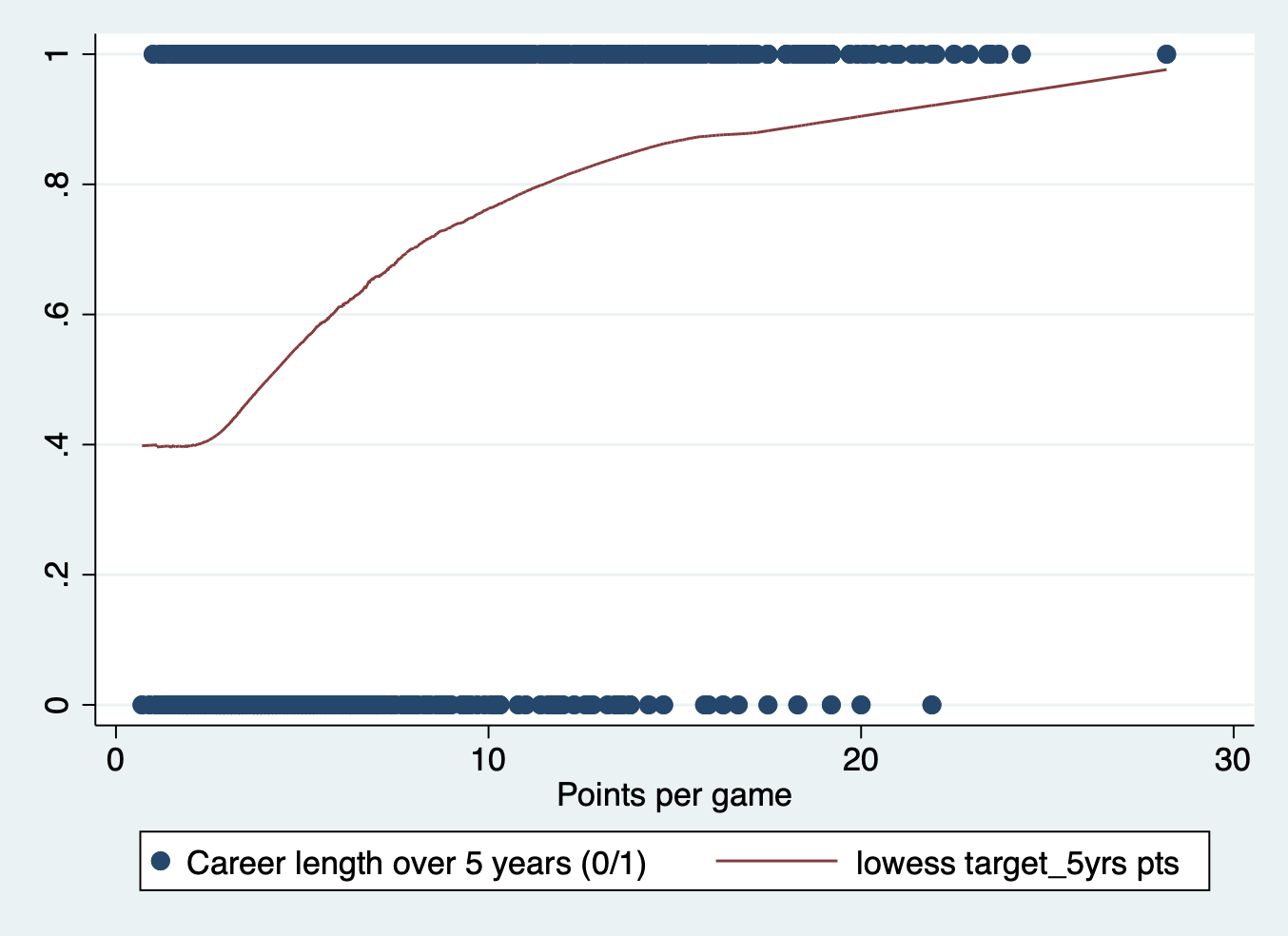
STEP 2: Run your models
There is only one command to run a normal probit model in stata, the probit command.
Like with the other models we’ve learned, it is good practice to run the most basic model first without any other covariates. Then you can get a sense of how the effect has changed once you add in your control variables. Our key variable is average points per game.
probit target_5yrs pts, nologProbit regression Number of obs = 1,340
LR chi2(1) = 155.18
Prob > chi2 = 0.0000
Log likelihood = -812.15587 Pseudo R2 = 0.0872
------------------------------------------------------------------------------
target_5yrs | Coefficient Std. err. z P>|z| [95% conf. interval]
-------------+----------------------------------------------------------------
pts | .1162099 .0101929 11.40 0.000 .0962322 .1361875
_cons | -.4321148 .0713262 -6.06 0.000 -.5719117 -.292318
------------------------------------------------------------------------------And then run the full model with all your covariates. You can also add them one at a time or in groups, depending on how you anticipate each independent variable affecting your outcome and how it ties back to your research question.
probit target_5yrs pts gp fg p ast blk, nologProbit regression Number of obs = 1,329
LR chi2(6) = 268.70
Prob > chi2 = 0.0000
Log likelihood = -747.19655 Pseudo R2 = 0.1524
------------------------------------------------------------------------------
target_5yrs | Coefficient Std. err. z P>|z| [95% conf. interval]
-------------+----------------------------------------------------------------
pts | .0370395 .01465 2.53 0.011 .0083261 .065753
gp | .0220105 .0026555 8.29 0.000 .0168058 .0272151
fg | .0237958 .0072869 3.27 0.001 .0095138 .0380778
p | .0011584 .0026386 0.44 0.661 -.0040131 .0063298
ast | .0315016 .0372342 0.85 0.398 -.0414762 .1044794
blk | .3033653 .1299551 2.33 0.020 .0486579 .5580727
_cons | -2.444897 .3288523 -7.43 0.000 -3.089436 -1.800359
------------------------------------------------------------------------------STEP 3: Interpret your model
As you’ve seen, running the probit regression model is exactly the same as logistic regression. Unlike logistic regression, we only have the raw z-score coefficients and the probability interpretations (predicted probabilities and marginal effects) to interpret the model.
Z Score Units
This interpretation doesn’t communicate much, except to let you know whether the relationship of the effect is increasing or decreasing. Let’s interpret two of the coefficients:
Points per game: Each additional point scored per game is associated with a .037 increase in the z-score of having an NBA career longer than 5 years.
Blocks per game: Each additional block per game is associated with a .303 increase in the z-score of having an NBA career longer than 5 years.
Again, this doesn’t mean much, so we’ll pivot immediately to stating the results in terms of probability.
Marginal Effects
As usual, we have three approaches for producing marginal effects (at means, at representative values, and average marginal effects). For these examples we will use the average marginal effects approach to restate the coefficients in terms of probability.
Points per game: Each additional point scored per game is associated with a 0.012 (1.2%) increase in the probability of having an NBA career longer than 5 years.
margins, dydx(pts)Average marginal effects Number of obs = 1,329
Model VCE: OIM
Expression: Pr(target_5yrs), predict()
dy/dx wrt: pts
------------------------------------------------------------------------------
| Delta-method
| dy/dx std. err. z P>|z| [95% conf. interval]
-------------+----------------------------------------------------------------
pts | .0118006 .0046428 2.54 0.011 .0027009 .0209003
------------------------------------------------------------------------------Blocks per game: Each additional point scored per game is associated with a .097 (9.7%) increase in the probability of having an NBA career longer than 5 years.
margins, dydx(blk)Average marginal effects Number of obs = 1,329
Model VCE: OIM
Expression: Pr(target_5yrs), predict()
dy/dx wrt: blk
------------------------------------------------------------------------------
| Delta-method
| dy/dx std. err. z P>|z| [95% conf. interval]
-------------+----------------------------------------------------------------
blk | .0966506 .0412124 2.35 0.019 .0158757 .1774254
------------------------------------------------------------------------------Important Note: Remember while marginal effects can give us a single number for the effect of a one unit change in a given X variable, in logistic and probit regression the size of that change varies across the X distribution. The effect might be large on the front end of the distribution and small on the back end. That is where predicted probability plots come in. They visualize the effect over the whole range of X (or at least the points we specify).
Predicted Probability Plots
With predicted probability plots, we don’t calculate the change in probability but instead the overall predicted probability at certain values of our covariates. Again, we want to choose an X variable to display the predicted probabilities over and an approach to handling the other covariates (at means, at representative values, or average predicted probabilities). I’ll use predicted probabilities at means for all of these plots.
Predicted probabilities at different levels of pts
margins, at(pts = (0(5)25)) atmeans
marginsplot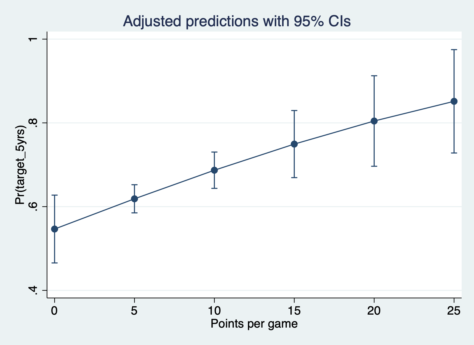
Predicted probabilities at different levels of blk
margins, at(blk = (0(.75)4)) atmeans
marginsplot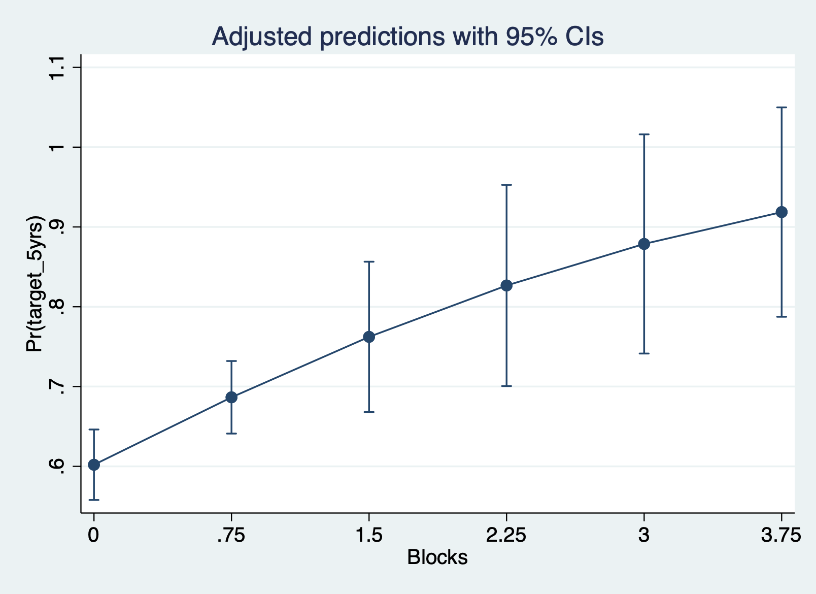
STEP 4: Check your assumptions
The outcome is binary
This is another logic check. Are we using a binary outcome in this analysis? Yes a player either does or does not have a career longer than 5 years.
The z-score outcome and x variables have a linear relationship
We can check this assumption by predicting the probit (aka outcome in z-score units), saving them to our dataset, and then plotting them against each independent variable. Here is what the scatter plot of the predicted log odds vs pts like with a lowess line.
predict probit, xb
scatter probit pts || lowess probit pts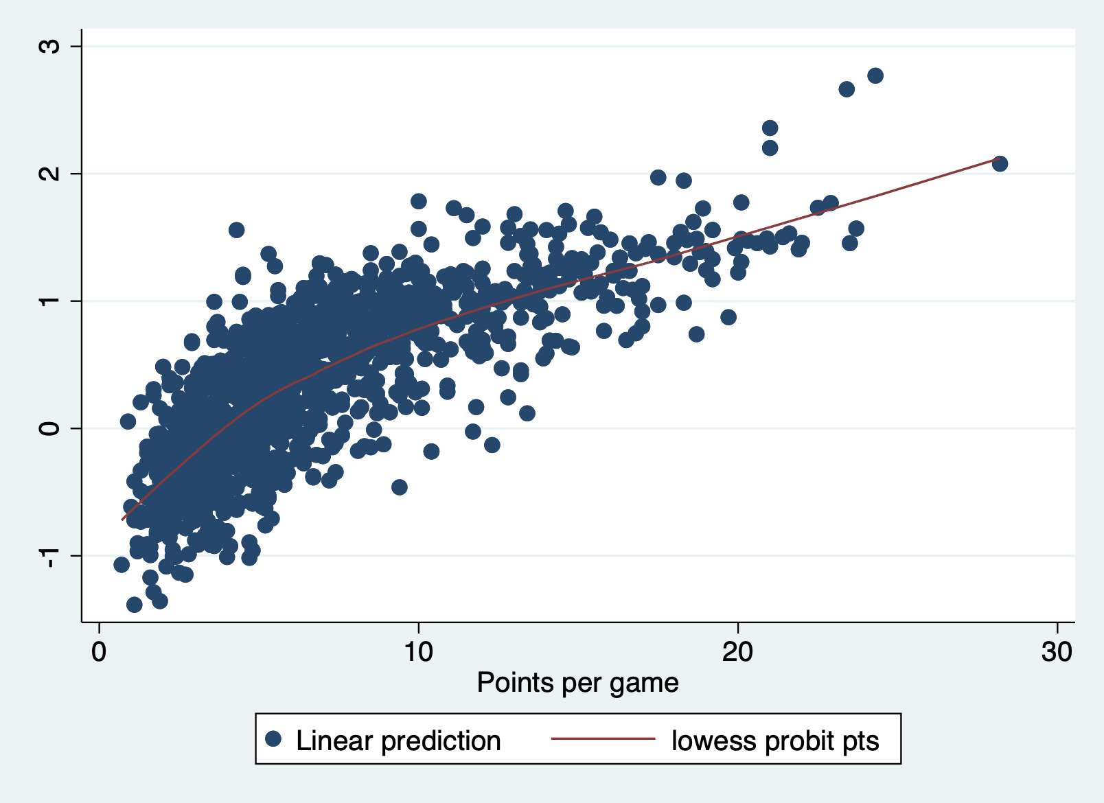
It has a little bend at the beginning, but not enough to concern me.
Normally distributed errors
Unlike logistic regression, we have to check whether the errors follow a normal distribution. We can do this the same way we do in linear regression.
First predict your errors, then plot them as a histogram.
predict r1
hist r1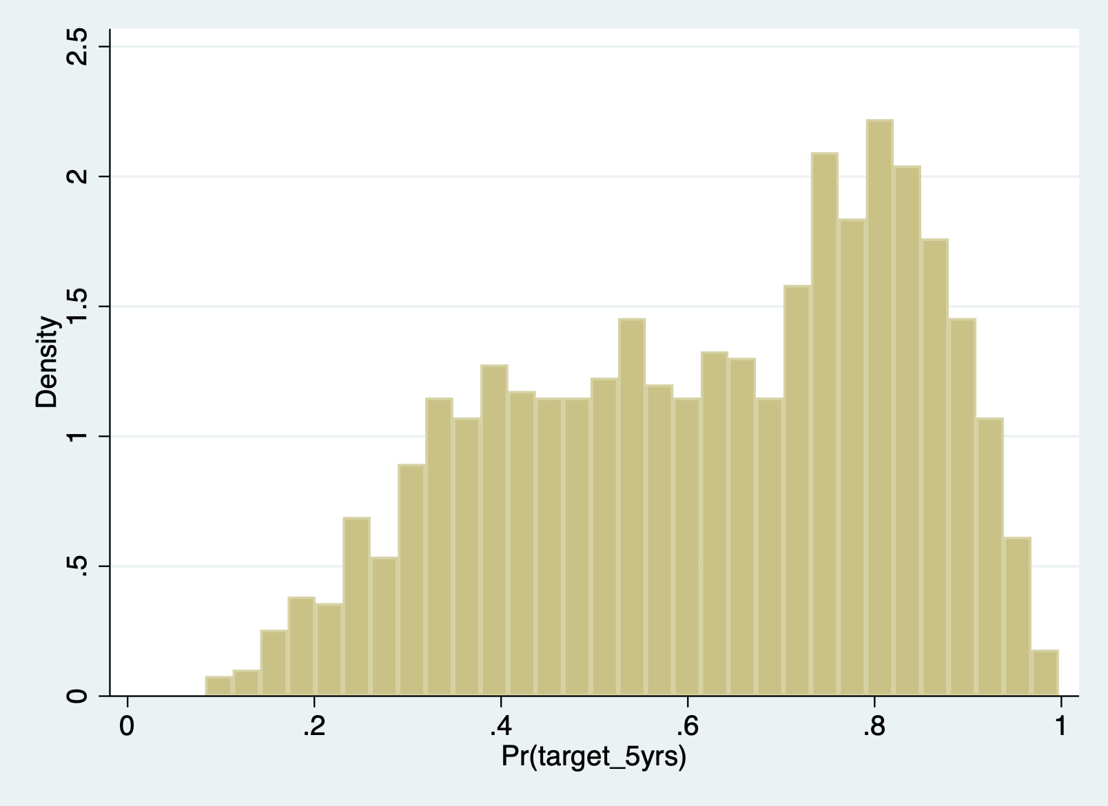
You can also look at the Q-Q plot. This plot graphs the normal distribution as a straight line. The further the points deviate from that line, the less normal the errors are.
qnorm r1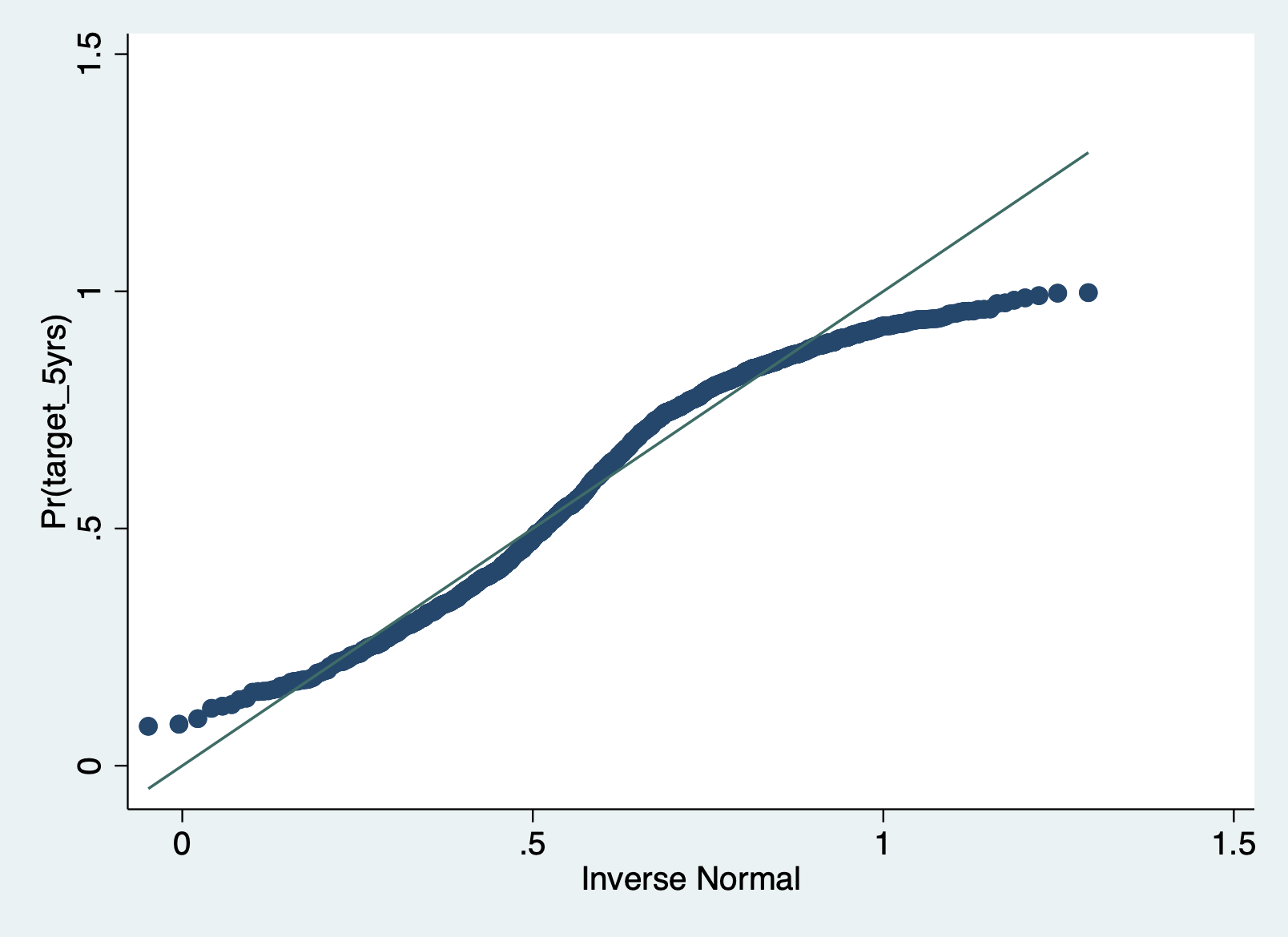
Errors are independent
This is another logic check. Do we have any clusters in this dataset? Well, if we had the team the player is on, that would be a cluster we would want to account for. Teams have the same schedule, the same teammates, and other potential similarities that would make their outcomes look more similar. Because we don’t have that variable in this dataset, we cannot account for it and have to decide how we think that clustering would change our results.
Multicolinearity
You may remember from linear regression that we can test for multicollinearity by calculating the variance inflation factor (VIF) for each covariate after the regression. Unfortunately, we can’t just use vif after the probit command. We can use this user written package instead.
First install the collin command if you haven’t yet:
net describe collin, from(https://stats.idre.ucla.edu/stat/stata/ado/analysis)
net install collin
And then run the collin command with all your covariates:
collin pts gp fg p ast blk(obs=1,329)
Collinearity Diagnostics
SQRT R-
Variable VIF VIF Tolerance Squared
----------------------------------------------------
pts 2.37 1.54 0.4214 0.5786
gp 1.53 1.24 0.6554 0.3446
fg 1.44 1.20 0.6924 0.3076
p 1.28 1.13 0.7825 0.2175
ast 1.85 1.36 0.5416 0.4584
blk 1.55 1.25 0.6435 0.3565
----------------------------------------------------
Mean VIF 1.67
Cond
Eigenval Index
---------------------------------
1 5.5363 1.0000
2 0.6868 2.8391
3 0.3789 3.8226
4 0.2512 4.6944
5 0.1017 7.3779
6 0.0382 12.0429
7 0.0068 28.4326
---------------------------------
Condition Number 28.4326
Eigenvalues & Cond Index computed from scaled raw sscp (w/ intercept)
Det(correlation matrix) 0.2046We’re looking for any VIF over 10, and we are good!