4 Logistic Regression (Stata)
4.1 Lab Overview
This web page provides a brief overview of logistic regression and a detailed explanation of how to run this type of regression in Stata. Download the script file to execute sample code for logistic regression. The last section of the script will ask you to apply the code you’ve learned with a simple example.
Research Question: What rookie year statistics are associated with having an NBA career longer than 5 years?
Lab Files
Data:
Download nba_rookie.dta
Script File:
Download lab2_LR.do
Script with answers to application question:
Download lab2_LR_w.answers.do
4.2 Logistic Regression Review
In logistic regression you are predicting the log-odds of your outcome as a function of your independent variables. To understand why our dependent variable becomes the log-odds of our outcome, let’s take a look at the binomial distribution.
Binary outcomes follow what is called the binomial distribution, whereas our outcomes in normal linear regression follow the normal distribution. In this scenario we are assuming that the probabilities following this binomial distribution fall on a logistic curve. It looks somewhat like an “S,” in contrast to the straight line we are used to seeing in linear regression.
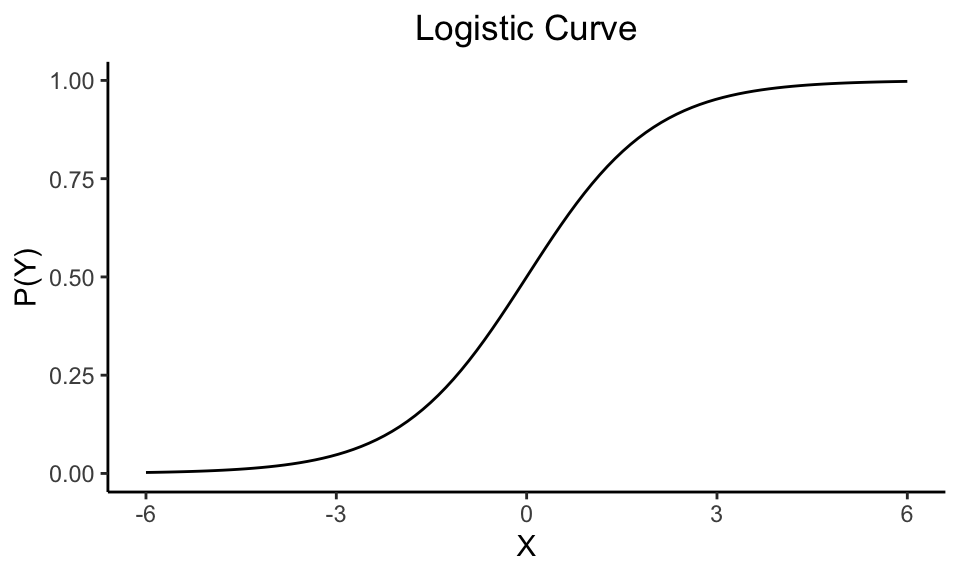
This distribution says that the probability of an event occurring \(P(Y=1)\) follows the logistic equation, where \(X\) is your independent variable. I promise there is math behind this that makes it all make sense, but for this class you can take my word for.
\[P(Y=1) = \displaystyle \frac{e^{\beta_0 + \beta_1X_1 + ... \beta_kX_k}}{1 + e^{\beta_0 + \beta_1X_1 + ... \beta_kX_k}}\]
But how in the world are we supposed use this equation in a regression?
Well, you might spot our handy linear equation in there (\(\beta_0 + \beta_1X_1 + ... \beta_kX_k\)). We want to be able to predict our outcome by adding together the effects of all our covariates using that linear equation. If we solve for that familiar equation we get:
\[\ln(\displaystyle \frac{P}{1-P}) = \beta_0 + \beta_1X_1 + ... \beta_kX_k\] Now that’s more like it! On the right side of the equals sign we have our familiar linear equation. The connection to the linear equation is why both logistic regression and normal linear regression are part of the same family: generalized linear models. On the left side of the equals sign we have log odds, which literally means “the log of the odds.” And as a reminder odds equals the probability of success (\(P\)) divided by the probability of failure (\(1-P\)).
4.2.1 Interpreting Log Odds – the Odds Ratio!
A one unit change in X is associated with a one unit change
in the log-odds of Y.
Running a logistic regression in Stata is going to be very similar to running a linear regression. The big difference is we are interpreting everything in log odds. Your coefficients are all in log odds units. Except…you are pretty much never going to describe something in terms of log odds. You will want to transform it into a (drum roll)…odds ratio.
An odds ratio (OR) is the odds of A over the odds of B. Let’s see how that works with a concrete example.
Example: The odds ratio for women vs men graduating from high school is 1.2.
Interpretation: Women are 1.2x more likely to graduate from high school than men.
Odds ratio makes interpreting coefficients in logistic regression very intuitive. Here’s a continuous variable example.
Example: The odds ratio for the effect of mother’s education on whether their child graduates high school is 1.05.
Interpretation: For every additional year of a mother’s education, a child is 1.05 times more likely to graduate from high school.
How do you go from a log odds to an odds ratio?
All you have to do to go from log odds to an odds ratio is “undo” the log part of log-odds. We do this by exponentiating exp() our coefficients, aka…
\[ e^\beta\]
So if the coefficient sex in a linear regression of high school graduation is 0.183…
\[ e^{0.183} = 1.2\]
And that is your odds ratio. In Stata you can use a command that automatically displays the odds ratios for each coefficient, no math necessary!
4.2.2 Assumptions of the model
(1) The outcome is binary
A binary variable has only two possible response categories. It is often referred to as present/not present or fail/success. Examples include: male/female, yes/no, pass/fail, drafted/not drafted, and many more!
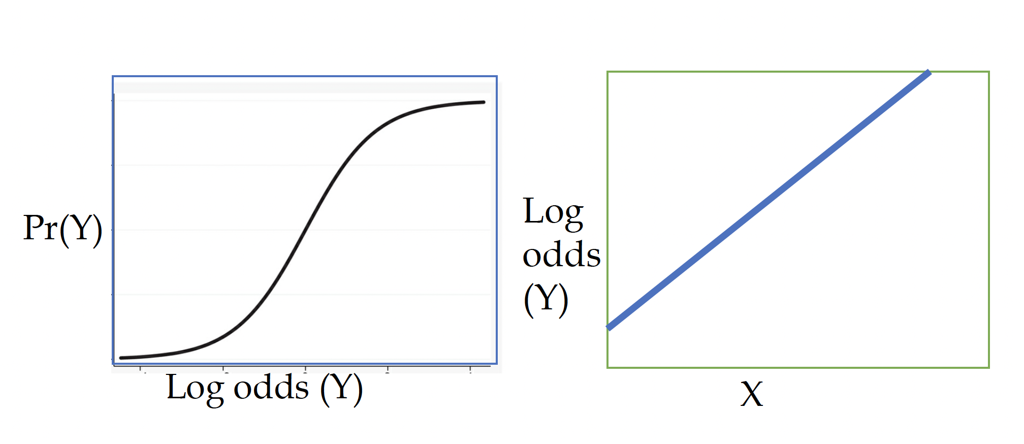
(2) The log-odds of the outcome and independent variable have a linear relationship
Although a smoothing line of your raw data will often reveal an s-shaped relationship between the outcome and explanatory variable, the log-odds of the outcome vs the explanatory variable should have a linear relationship. In the plots below, the blue box on the right shows the raw s-shape and the green plot on the left shows the transformed, linear log-odds relationship.
How to address it?
Like a linear regression, you can play around with squared and cubed terms to see if they address the curved relationship in your data.
(3) Errors are independent
Like linear regression we don’t want to have obvious clusters in our data. Examples of clusters would be multiple observations from the same person at different times, multiple observations withing schools, people within cities, and so on.
How to address it?
If you have a variable identifying the cluster (e.g., year, school, city, person), you can run a logistic regression adjusted for clustering using cluster-robust standard errors (rule of thumb is to have 50 clusters for this method). However, you may also want to consider learning about and applying a hierarchical linear model.
(4) No severe multicolinearity
This is another carryover from linear regression. Multicollineary can throw a wrench in your model when one or more independent variables are correlated to one another.
How to address it?
Run a VIF (variance inflation factor) to detect correlation between your independent variables. Consider dropping variables or combining them into one factor variable.
Differences to linear regression assumptions
Logistic regression and linear regression belong to the same family of models, but logistic regression DOES NOT require an assumption of homoskedasticity or that the errors be normally distributed.
4.2.3 Pros and Cons of the model
Pros:
- You can interpret an odds ratio as how many more times someone is likely to experience the outcome (e.g., nba players with high scoring averages are 1.5 times more likely to have a career over five years).
- Logistic regression are the most common model used for binary outcomes.
Cons:
- Odds ratios and log-odds are not as straightforward to interpret as the outcomes of a linear probability model.
- It assumes linearity between log-odds outcome and explanatory variables.
4.3 Running a logistic regression in Stata
Now we will walk through running and interpreting a logistic regression in Stata from start to finish. The trickiest piece of this code is interpretation via predicted probabilities and marginal effects.
These steps assume that you have already:
- Cleaned your data.
- Run descriptive statistics to get to know your data in and out.
- Transformed variables that need to be transformed (logged, squared, etc.)
We will be running a logistic regression to see what rookie characteristics are associated with an NBA career greater than 5 years.
STEP 1: Plot your outcome and key independent variable
This step isn’t strictly necessary, but it is always good to get a sense of your data and the potential relationships at play before you run your models.
To get a sense of the relationship in a logistic regression you can plot your outcome over your key independent variable. You can also do this with any other independent variable in your model.
scatter target_5yrs pts || lowess target_5yrs pts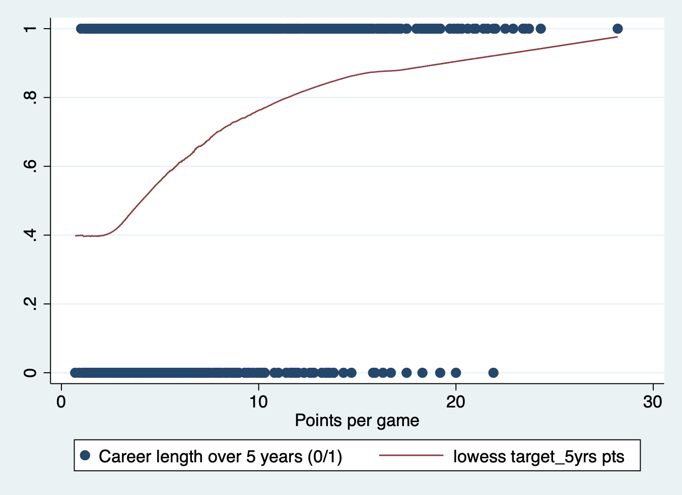
STEP 2: Run your models
You can run this with the logit command or the logistic command. Because it is more common to present odds ratios, I will go ahead and use the logistic command.
Like with linear regression and linear probability models, it is good practice to run the most basic model first without any other covariates. Then you can get a sense of how the effect has changed once you add in your control variables. Our key variable is average points per game.
logistic target_5yrs ptsLogistic regression Number of obs = 1,340
LR chi2(1) = 159.18
Prob > chi2 = 0.0000
Log likelihood = -810.15675 Pseudo R2 = 0.0895
------------------------------------------------------------------------------
target_5yrs | Odds ratio Std. err. z P>|z| [95% conf. interval]
-------------+----------------------------------------------------------------
pts | 1.226937 .0232817 10.78 0.000 1.182144 1.273428
_cons | .4579115 .0562467 -6.36 0.000 .3599364 .5825556
------------------------------------------------------------------------------
Note: _cons estimates baseline odds.And then run the full model with all your covariates. You can also add them one at a time or in groups, depending on how you anticipate each independent variable affecting your outcome and how it ties back to your research question.
logistic target_5yrs pts gp fg p ast blkLogistic regression Number of obs = 1,329
LR chi2(6) = 268.31
Prob > chi2 = 0.0000
Log likelihood = -747.39055 Pseudo R2 = 0.1522
------------------------------------------------------------------------------
target_5yrs | Odds ratio Std. err. z P>|z| [95% conf. interval]
-------------+----------------------------------------------------------------
pts | 1.068487 .0275617 2.57 0.010 1.01581 1.123896
gp | 1.036207 .0046205 7.98 0.000 1.027191 1.045303
fg | 1.039597 .0127005 3.18 0.001 1.015 1.06479
p | 1.001582 .0043688 0.36 0.717 .9930561 1.010182
ast | 1.053761 .0676164 0.82 0.414 .9292305 1.194981
blk | 1.714731 .3924485 2.36 0.018 1.09492 2.685403
_cons | .0181963 .0100923 -7.22 0.000 .0061359 .0539622
------------------------------------------------------------------------------
Note: _cons estimates baseline odds.STEP 3: Interpret your model
As you’ve seen, running the logistic regression model itself isn’t that much different than a linear regression. What gets more complicated is interpretation. There are four ways you can interpret a logistic regression:
- Log odds (the raw output given by a logistic regression)
- Odds ratios
- Predicted probabilities
- Marginal effects
This lab will cover the last three. A change in log odds is a pretty meaningless unit of measurement. So you will want to report your results in at least one of these three forms. This lab cannot cover every variation of running predicted probability and marginal effects in Stata. We will practice margins in a future lab, but for now try to wrap your mind around these basic variations.
Odds Ratios
Remember, we go from log odds to odds ratios by exponentiating the raw log odds coefficients. But logistic has already done that for us. Let’s interpret two of the coefficients:
Points per game: Each additional point scored per game makes a player 1.07 times more likely to have an NBA career longer than 5 years OR the odds a player has an NBA career longer than 5 years increases the odds by 7%.
Blocks per game: Each additional block per game makes a player 1.71 times more likely to have an NBA career longer than 5 years OR the odds a player has an NBA career longer than 5 years increases the odds by 71%.
Predicted Probability Plots
Here we return to our good friend the margins command. In linear regression, the margins command produces predicted values. So if the outcome of the linear regression was income, the predicted value would be some income value based on the model. In logistic regression, the outcome of the margins command is a predicted probability. Our outcome ranges from 0 to 1, and the predicted probability tells us the likelihood the outcome will occur based on the model. You can then plot those predicted probabilities to visualize the findings from the model. There are three approaches to calculating these probabilities. Why are there multiple approaches, because we get predicted probabilities/values from plugging in values to our regression equation. Stata needs to know what value to plug into each variable in our equation. Let’s look at the three approaches to doing those calculations…
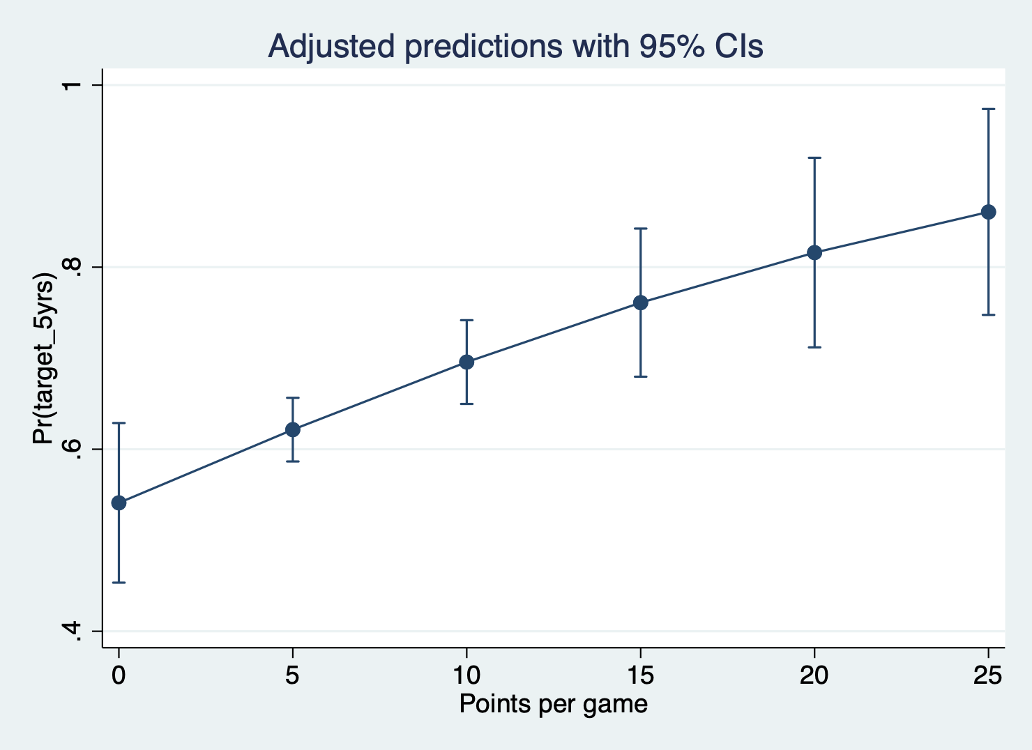
(1) Predicted probabilities with all other variables held AT MEANS
In this method, you choose an explanatory variable you want to plot your probabilities over and plug in the average value for each of the other variables. For example, here we ask Stata to calculate the predicted probabilities for our outcome over the range of our pts variable. We have to specify which values of pts we want Stata to calculate, and then we tell Stata to put the other variables at means.
What values of pts do we want to get probabilities for? I’m using the (start(interval)end) format to predict values from 0 (start) to 25 (end) at intervals of 5.
margins, at(pts = (0(5)25)) atmeans
marginsplot
Adjusted predictions Number of obs = 1,329
Model VCE: OIM
Expression: Pr(target_5yrs), predict()
1._at: pts = 0
gp = 60.40256 (mean)
fg = 44.11753 (mean)
p = 19.30813 (mean)
ast = 1.558992 (mean)
blk = .36614 (mean)
2._at: pts = 5
gp = 60.40256 (mean)
fg = 44.11753 (mean)
p = 19.30813 (mean)
ast = 1.558992 (mean)
blk = .36614 (mean)
3._at: pts = 10
gp = 60.40256 (mean)
fg = 44.11753 (mean)
p = 19.30813 (mean)
ast = 1.558992 (mean)
blk = .36614 (mean)
4._at: pts = 15
gp = 60.40256 (mean)
fg = 44.11753 (mean)
p = 19.30813 (mean)
ast = 1.558992 (mean)
blk = .36614 (mean)
5._at: pts = 20
gp = 60.40256 (mean)
fg = 44.11753 (mean)
p = 19.30813 (mean)
ast = 1.558992 (mean)
blk = .36614 (mean)
6._at: pts = 25
gp = 60.40256 (mean)
fg = 44.11753 (mean)
p = 19.30813 (mean)
ast = 1.558992 (mean)
blk = .36614 (mean)
------------------------------------------------------------------------------
| Delta-method
| Margin std. err. z P>|z| [95% conf. interval]
-------------+----------------------------------------------------------------
_at |
1 | .5410642 .0447506 12.09 0.000 .4533546 .6287739
2 | .6214831 .0178435 34.83 0.000 .5865106 .6564557
3 | .6957347 .0234751 29.64 0.000 .6497244 .741745
4 | .7610217 .0415165 18.33 0.000 .6796508 .8423925
5 | .8160046 .053124 15.36 0.000 .7118834 .9201258
6 | .8606537 .0577089 14.91 0.000 .7475464 .973761
------------------------------------------------------------------------------
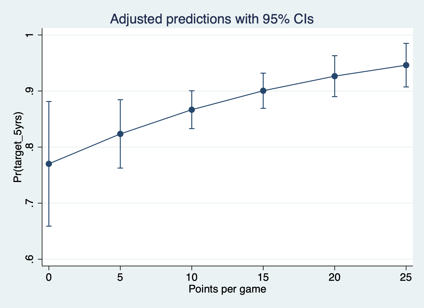
(2) Predicted probabilities with all other variables at REPRESENTATIVE VALUES
In this method, you choose an explanatory variable you want to plot your probabilities over and plug in representative values for the other variables. Remember, there is no “average” person. So maybe you are predicting the probability of high school graduation and want to show the probability for a low-income student with a lot of adverse childhood experiences. You specify the values of the main explanatory variable you want to predict over and fill in the other variables with the values corresponding to that profile.
Let’s say we think Michael Finley is a mid-level rookie player (this is totally made up, I know very little about basketball). So we’ll plug in his values to get our predicted probability.
margins, at(pts = (0(5)25) gp == 82 fg == 47.6 p == 32.8 ///
                                ast == 3.5 blk == .4)
marginsplot
> ast == 3.5 blk == .4)
Adjusted predictions Number of obs = 1,329
Model VCE: OIM
Expression: Pr(target_5yrs), predict()
1._at: pts = 0
gp = 82
fg = 47.6
p = 32.8
ast = 3.5
blk = .4
2._at: pts = 5
gp = 82
fg = 47.6
p = 32.8
ast = 3.5
blk = .4
3._at: pts = 10
gp = 82
fg = 47.6
p = 32.8
ast = 3.5
blk = .4
4._at: pts = 15
gp = 82
fg = 47.6
p = 32.8
ast = 3.5
blk = .4
5._at: pts = 20
gp = 82
fg = 47.6
p = 32.8
ast = 3.5
blk = .4
6._at: pts = 25
gp = 82
fg = 47.6
p = 32.8
ast = 3.5
blk = .4
------------------------------------------------------------------------------
| Delta-method
| Margin std. err. z P>|z| [95% conf. interval]
-------------+----------------------------------------------------------------
_at |
1 | .7701667 .0567214 13.58 0.000 .6589948 .8813385
2 | .8235335 .0311068 26.47 0.000 .7625652 .8845017
3 | .8666541 .0172264 50.31 0.000 .8328909 .9004173
4 | .9005109 .0159995 56.28 0.000 .8691524 .9318693
5 | .9265004 .0186286 49.74 0.000 .889989 .9630117
6 | .946107 .0198164 47.74 0.000 .9072674 .9849465
------------------------------------------------------------------------------
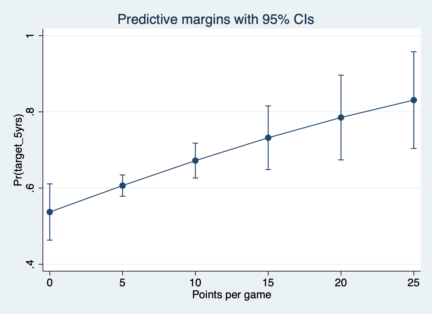
(3) AVERAGE predicted probabilities
This is the most common method of predicting probabilities and the default in Stata. In this method, you choose an explanatory variable you want to plot your probabilities over. Stata plugs in the actual observed values for every observation, calculates the probability over your specified range of values, and then calculates the average probability across all observations. You don’t have to specify anything except for the values of your explanatory variable to calculate probabilities for.
margins, at(pts = (0(5)25))
marginsplot
Predictive margins Number of obs = 1,329
Model VCE: OIM
Expression: Pr(target_5yrs), predict()
1._at: pts = 0
2._at: pts = 5
3._at: pts = 10
4._at: pts = 15
5._at: pts = 20
6._at: pts = 25
------------------------------------------------------------------------------
| Delta-method
| Margin std. err. z P>|z| [95% conf. interval]
-------------+----------------------------------------------------------------
_at |
1 | .5371862 .0376362 14.27 0.000 .4634206 .6109518
2 | .6065213 .0142551 42.55 0.000 .5785819 .6344608
3 | .6720795 .0233919 28.73 0.000 .6262321 .7179268
4 | .7320496 .0425491 17.20 0.000 .648655 .8154443
5 | .7851854 .0567287 13.84 0.000 .6739993 .8963716
6 | .8308522 .064745 12.83 0.000 .7039542 .9577501
------------------------------------------------------------------------------
Marginal Effects
Now we are staying with our friend margins, but we’re going to move from calculating the probability to calculating how the probability changes when we increase one unit of an explanatory variable. Because probabilities aren’t linear, the effect of a one-unit change will be different as we move across the range of X values. We can use these three approaches to get a single value answer for how a one unit change in X affects the probability of Y. We do this by specifying dydx() in our margins command. Again, there are three ways to do this calculation. We’re plugging values in the equation again, but using calculus to find this marginal effect. The command for the three approaches are very similar to the above, with the addition of dydx().
(1) Marginal effect of a one unit change in X AT MEANS (MEM)
Here you specify which variable you want to find the marginal effect for inside of dydx(), and tell Stata to plug in the mean for each of the other X variables.
Get the marginal effect of average points per game, at means:
margins, dydx(pts) atmeansConditional marginal effects Number of obs = 1,329
Model VCE: OIM
Expression: Pr(target_5yrs), predict()
dy/dx wrt: pts
At: pts = 6.820166 (mean)
gp = 60.40256 (mean)
fg = 44.11753 (mean)
p = 19.30813 (mean)
ast = 1.558992 (mean)
blk = .36614 (mean)
------------------------------------------------------------------------------
| Delta-method
| dy/dx std. err. z P>|z| [95% conf. interval]
-------------+----------------------------------------------------------------
pts | .0150823 .005845 2.58 0.010 .0036263 .0265384
------------------------------------------------------------------------------Interpretation: Holding all variables at their means, a one unit increase in avg points per game is associated with a 0.015 increase in the probability of an NBA career beyond 5 years.
You can also see all the marginal effects at means for all X variables:
margins, dydx(*) atmeansConditional marginal effects Number of obs = 1,329
Model VCE: OIM
Expression: Pr(target_5yrs), predict()
dy/dx wrt: pts gp fg p ast blk
At: pts = 6.820166 (mean)
gp = 60.40256 (mean)
fg = 44.11753 (mean)
p = 19.30813 (mean)
ast = 1.558992 (mean)
blk = .36614 (mean)
------------------------------------------------------------------------------
| Delta-method
| dy/dx std. err. z P>|z| [95% conf. interval]
-------------+----------------------------------------------------------------
pts | .0150823 .005845 2.58 0.010 .0036263 .0265384
gp | .0080978 .0010224 7.92 0.000 .006094 .0101017
fg | .0088414 .0027907 3.17 0.002 .0033718 .0143111
p | .00036 .0009933 0.36 0.717 -.0015868 .0023067
ast | .0119226 .0146065 0.82 0.414 -.0167057 .0405509
blk | .1227768 .0518679 2.37 0.018 .0211176 .2244361
------------------------------------------------------------------------------(2) Marginal effect of one unit change in X at REPRESENTATIVE VALUES (MER)
Now for this approach we specify the variable we want to find the marginal effect for and then specify the specific values for the other variables that correspond with our “representative case.” We’ll use Michael Finley’s profile again.
Get the marginal effect of average points per game with representative values:
margins, dydx(pts) at (gp == 82 fg == 47.6 p == 32.8 ///
                        ast == 3.5 blk == .4)
> ast == 3.5 blk == .4)
Average marginal effects Number of obs = 1,329
Model VCE: OIM
Expression: Pr(target_5yrs), predict()
dy/dx wrt: pts
At: gp = 82
fg = 47.6
p = 32.8
ast = 3.5
blk = .4
------------------------------------------------------------------------------
| Delta-method
| dy/dx std. err. z P>|z| [95% conf. interval]
-------------+----------------------------------------------------------------
pts | .0089695 .0042941 2.09 0.037 .0005532 .0173857
------------------------------------------------------------------------------Intepretation: For a player with these stats in their rookie year, a one unit increase in avg points per game is associated with a 0.008 increase in the probability of an NBA career past 5 years.
(3) AVERAGE marginal effects (AME)
Again, this is the most common/default method to produce marginal effects in Stata. You only have to specify the variable you want to calculate the marginal effects for.
Get the average marginal effect for points per game with representative values:
margins, dydx(pts)Average marginal effects Number of obs = 1,329
Model VCE: OIM
Expression: Pr(target_5yrs), predict()
dy/dx wrt: pts
------------------------------------------------------------------------------
| Delta-method
| dy/dx std. err. z P>|z| [95% conf. interval]
-------------+----------------------------------------------------------------
pts | .0126177 .0048798 2.59 0.010 .0030535 .022182
------------------------------------------------------------------------------Interpretation: Holding all other variables at their observed values, on average a one unit increase in average points per game is associated with a 0.012 increase in the probability of an NBA career past 5 years.
STEP 4: Check your assumptions
The outcome is binary
This is another logic check. Are we using a binary outcome in this analysis? Yes a player either does or does not have a career longer than 5 years.
The log-odds of the outcome and independent variable have a linear relationship
We can check this assumption by predicting the logits (aka the log odds), saving them to our dataset, and then plotting them against each independent variable. Here is what the scatter plot of the predicted log odds vs pts like with a lowess line.
predict logits, xb
scatter logits pts || lowess logits pts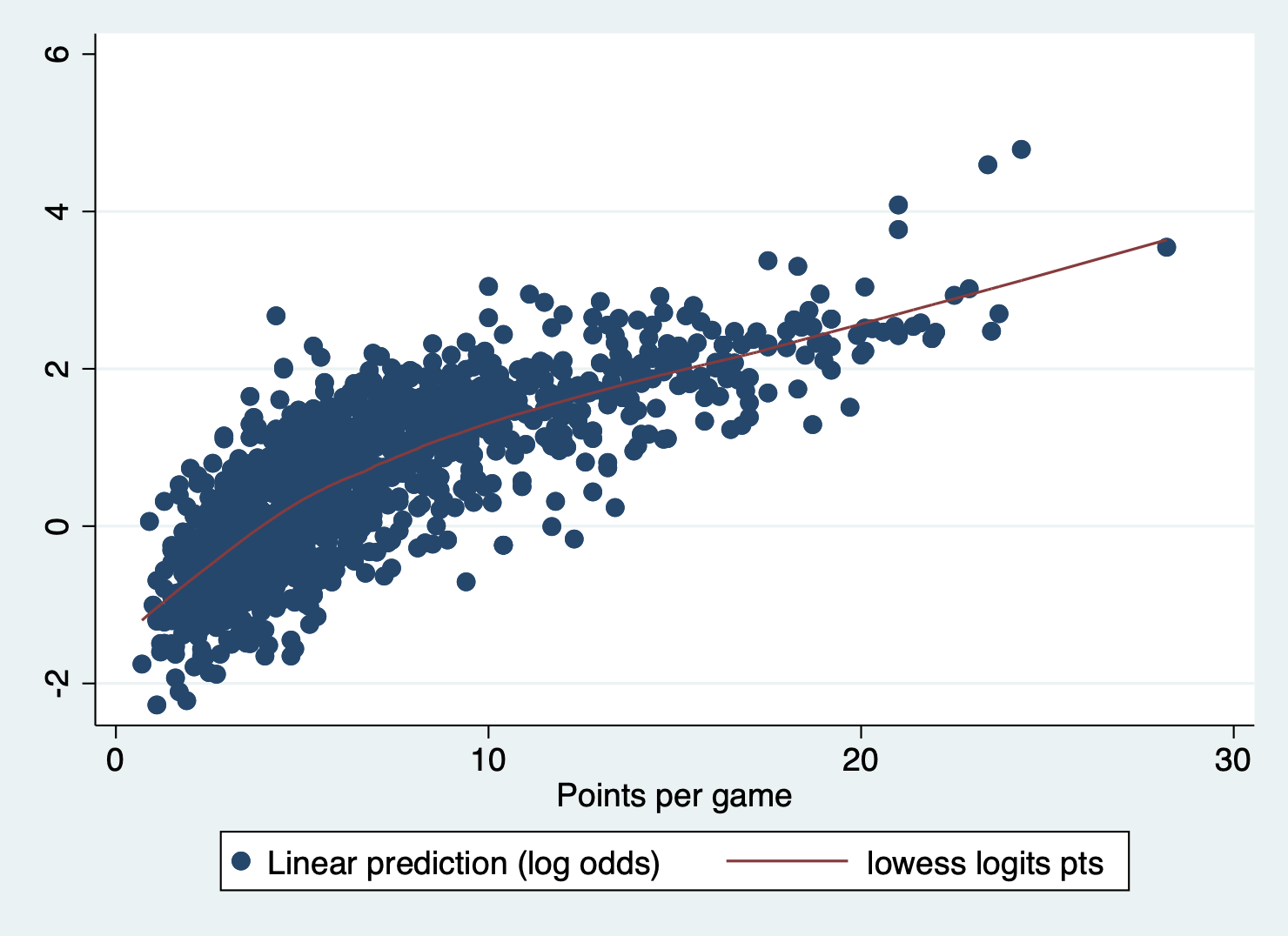
It has a little bend at the beginning, but not enough to concern me.
Errors are independent
This is another logic check. Do we have any clusters in this dataset? Well, if we had the team the player is on, that would be a cluster we would want to account for. Teams have the same schedule, the same teammates, and other potential similarities that would make their outcomes look more similar. Because we don’t have that variable in this dataset, we cannot account for it and have to decide how we think that clustering would change our results.
No severe multicolinearity
You may remember from linear regression that we can test for multicollinearity by calculating the variance inflation factor (VIF) for each covariate after the regression. Unfortunately, we can’t just use vif after the logistic command. We can use this user written package instead.
First install the collin command:
net describe collin, from(https://stats.idre.ucla.edu/stat/stata/ado/analysis)
net install collin
And then run the collin command with all your covariates:
collin pts gp fg p ast blk(obs=1,329)
Collinearity Diagnostics
SQRT R-
Variable VIF VIF Tolerance Squared
----------------------------------------------------
pts 2.37 1.54 0.4214 0.5786
gp 1.53 1.24 0.6554 0.3446
fg 1.44 1.20 0.6924 0.3076
p 1.28 1.13 0.7825 0.2175
ast 1.85 1.36 0.5416 0.4584
blk 1.55 1.25 0.6435 0.3565
----------------------------------------------------
Mean VIF 1.67
Cond
Eigenval Index
---------------------------------
1 5.5363 1.0000
2 0.6868 2.8391
3 0.3789 3.8226
4 0.2512 4.6944
5 0.1017 7.3779
6 0.0382 12.0429
7 0.0068 28.4326
---------------------------------
Condition Number 28.4326
Eigenvalues & Cond Index computed from scaled raw sscp (w/ intercept)
Det(correlation matrix) 0.2046We’re looking for any VIF over 10, and we are good!
A note on R-squared
We will discuss this more in our lab on comparing models, but R-squared statistics are more complicated with linear regression. They cannot be calculated in the same way as a linear regression because the estimation procedures are different. People have come up with many different ways to calculate an R-squared statistic. Stata shows “Pseudo R-squared” or Mcfadden’s R-squared, but there are other ways of evaluating how well your model fits the data for logistic regressions.
4.4 Apply this model on your own
Run a new regression using
target_5yrsas your outcome and three new independent variables. You can uselogitorlogistic.Calculate and plot the predicted probabilities at different levels of ONE independent variable, holding the other two at means.
Calculate the average marginal effect of ONE of your independent variables