2 Linear Probability Models (Stata)
2.1 Lab Overview
Today you will be learning the first regression method you can use to predict a binary outcome. This web page includes a more detailed explanation of Linear Probability Models in Stata and a script file you will execute to learn the basics of running this new model. The last section of the script will ask you to apply the code you’ve learned with a simple example.
Research Question: What characteristics of passengers are associated with survival on the Titanic?
Lab Files
Data:
Download titanic_df.dta
Script File:
Download lab1_LPM.do
Script with answers to application question:
Download lab1_LPM_w.answers.do
2.2 What is a Linear Probability Model (LPM)?
First, let’s review some of the basic characteristics of a Linear Probability Model (LPM):
LPM uses a normal OLS linear regression (ordinary least squares), but with a binary outcome rather than a continuous outcome.
A binary outcome is coded as 0 = not present, 1 = present. Sometimes binary outcomes are thought of as “success” or “failure.” Sometimes a binary outcome could be a characteristic. Some examples of binary outcomes are: graduating from high school, getting arrested, agreeing with a statement, getting a disease, and many more!
When you run a LPM, your interpretation of the regression results changes. Your coefficients now refers to the probability that an outcome occurs.
Probability of an event is always between 0 and 1, but a LPM can sometimes give us probabilities greater than 1.
The LPM is an alternative to logistic regression or probit regression. There are rarely big differences in the results between the three models.
This is the basic equation set up for a linear probability model:
\[P(Yi = 1|Xi) = \beta_0 \ + \ \beta_1X_{i,1} \ + \ \beta_2X_{i,2} + ... \beta_kX_{i,k} + \epsilon\]
- \(P(Yi = 1|Xi)\): The probability that the outcome is present (1 = present / 0 = not present)
- That probability is predicted as a linear function (meaning the effects of each coefficient are just added together to get the outcome probability).
- \(\beta_0\) - the intercept (or probability of all coefficients are 0).
- \(\beta_k\) - the probability associated with any covariate
- \(X_k\) - the value of the covariate
- \(\epsilon\) - the error (aka the difference between the predicted probability and the actual outcome [0/1])
- \(\beta_0\) - the intercept (or probability of all coefficients are 0).
Why should you care about this equation?
For each model we learn this quarter, I will break down how to understand the basic model equation. I do this for several reasons:
- Very practically, you will need to write out the equation for your model in the methods sections of your quantitative papers.
- It will help with your quantitative literacy when reading journal articles! I know I sometimes check out when I see an equation in an article that goes way over my head. This is a way to make yourself feel like a smarty pants.
- It can help you wrap your mind around what a model is actually doing. Any model that we run is predicting an outcome as an equation, like a recipe. One part this variable plus one part that variable should equal this outcome. As we switch from model to model, the equation that we are using to predict outcomes will change.
2.2.1 Assumptions of the model
The assumptions of a LPM are pretty much the same as a normal linear regression. This means you need to consider each of these assumptions when you run a linear probability model on a binary outcome in your data.
1) Violation of the linearity assumption
LPM knowingly violates the assumption that there is a linear relationship between
the outcome and the covariates. If you run a lowess line, it often looks s-shaped.
2) Violation of the homoskedasticity assumption
Errors in a linear probability model will by nature have systematic heteroskedasticity. You can account for this by automatically using robust standard errors.
3) Normally distributed errors
Errors follow a normal distribution. This assumption only matters if you have a very small sample size.
4) Errors are independent
There is no potential clustering within your data. Examples would be data collected from withing a set of schools, within a set of cities, from different years, and so on.
5) X is not invariant
The covariates that you choose can’t all be the same value! You want variation so you can test to see how the outcome changes when the x value changes.
6) X is independent of the error term
There are no glaring instances of confounding in your model. This assumption is about unmeasured or unobserved variables that you might reasonably expect would be associated with your covariates and outcome. You can never fully rule this violation out, but you should familiarize yourself with other studies in your area to know what major covariates you should include.
7) Errors have a mean of 0 (at every level of X)
This is an assumption we did not cover last quarter. It essentially looks at whether your model is consistently over-estimating or under-estimating the outcomes. If the mean is positive, your model is UNDER-estimating the outcome (more of the errors are positive). If the mean is negative, your model is OVER-estimating the outcome.
Why didn’t we cover this assumption last quarter? Good Question! By including an intercept or constant in our regression (\(\beta_0\)), we force the errors to have a mean of 0, so we don’t have to worry about it. You will almost never run a regression without an intercept.
2.2.2 Pros and cons of the model
Pros:
- The LPM is simple to run if you already know how to run a linear regression.
- It is easy to interpret as a change in the probability of the outcome ocurring.
Cons:
- It violates two of the main assumptions of normal linear regression.
- You’ll get predict probabilities that can’t exist (i.e., they are above 1 or below 0).
2.3 Running a LPM in Stata
Now we will walk through running and interpreting a linear regression in Stata from start to finish. This will be relatively straightforward if you know how to run a linear regression in Stata, because we will be following basically the same steps. These steps assume that you have already:
- Cleaned your data.
- Run descriptive statistics to get to know your data in and out.
- Transformed variables that need to be transformed (logged, squared, etc.)
We will be running a LPM to see what personal characteristics are associated with surviving the Titanic shipwreck.
Step 1: Plot your outcome and key independent variable
Before you run your regression. Take a look at your outcome and key independent variables in a scatter plot with a lowess line to see if there may be a relationship between your variables. A flat line would indicate no relationship.
scatter survived port || lowess survived port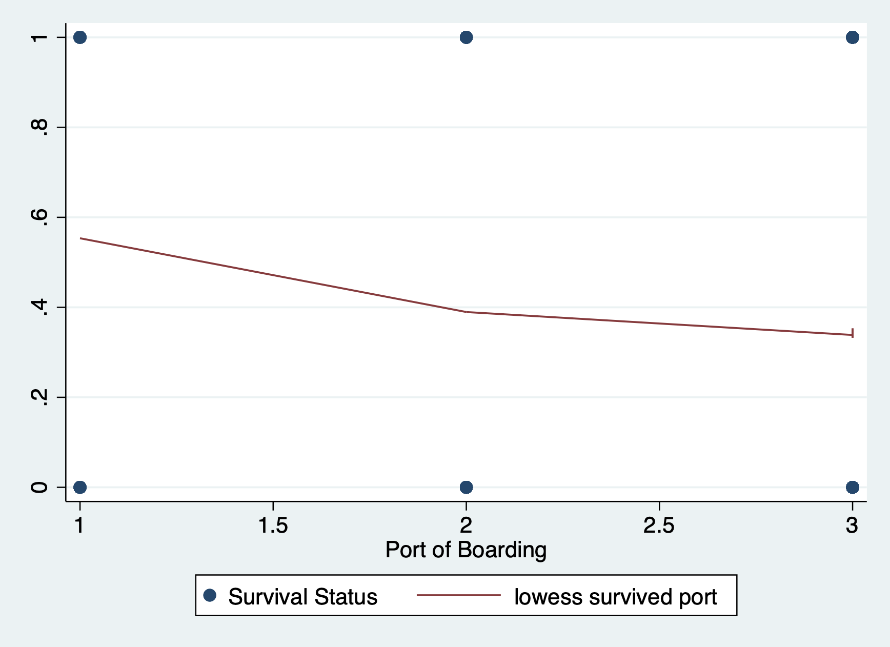
You can see that there is a classic curve to this relationship we will be seeing more as we learn other binary regression models this quarter.
Step 2: Run your model
First, you want to run a basic model with your outcome and key independent variable.
NOTE: We will be using robust standard errors because we know we will be violating the heteroskedasticity assumption.
regress survived i.port, robust Linear regression Number of obs = 889
F(2, 886) = 12.88
Prob > F = 0.0000
R-squared = 0.0298
Root MSE = .4795
------------------------------------------------------------------------------
| Robust
survived | Coefficient std. err. t P>|t| [95% conf. interval]
-------------+----------------------------------------------------------------
port |
Queenstown | -.163961 .0676383 -2.42 0.016 -.2967111 -.031211
Southampton | -.2166149 .0427093 -5.07 0.000 -.3004382 -.1327916
|
_cons | .5535714 .0384187 14.41 0.000 .4781692 .6289736
------------------------------------------------------------------------------Then you want to run your model with additional covariates.
regress survived i.port i.female log_fare, robust Linear regression Number of obs = 889
F(4, 884) = 157.61
Prob > F = 0.0000
R-squared = 0.3368
Root MSE = .3969
------------------------------------------------------------------------------
| Robust
survived | Coefficient std. err. t P>|t| [95% conf. interval]
-------------+----------------------------------------------------------------
port |
Queenstown | -.0869602 .0539718 -1.61 0.107 -.192888 .0189675
Southampton | -.1023845 .0367179 -2.79 0.005 -.1744489 -.0303201
|
female |
Female | .4960477 .0322092 15.40 0.000 .4328324 .5592631
log_fare | .090448 .0146489 6.17 0.000 .0616974 .1191986
_cons | .0224237 .0580422 0.39 0.699 -.0914929 .1363404
------------------------------------------------------------------------------Step 3: Interpret your model
There are three ways we can interpret and communicate the results of our model:
- Interpretation of the coefficients
- Plot the regression line
- Plot our predicted probabilities (aka margins)
Interpret coefficients
The reason people like the LPM is that the coefficients are so straightforward to interpret. A one unit change in X is associated with a change in the probability that Y occurs. Remember our outcome is binary: yes the outcome occurs or no it does not. It often makes the most sense to interpret that probability change as a change in the percent probability of our outcome occurring, so we multiply the coefficient by 100.
To do basic math with our coefficients in helps to know how Stata labels them. You can find this out by pulling up your coefficient legend.
regress, coeflegendLinear regression Number of obs = 889
F(4, 884) = 157.61
Prob > F = 0.0000
R-squared = 0.3368
Root MSE = .3969
------------------------------------------------------------------------------
survived | Coefficient Legend
-------------+----------------------------------------------------------------
port |
Queenstown | -.0869602 _b[2.port]
Southampton | -.1023845 _b[3.port]
|
female |
Female | .4960477 _b[1.female]
log_fare | .090448 _b[log_fare]
_cons | .0224237 _b[_cons]
------------------------------------------------------------------------------Let’s interpret each coefficient…
Port - Queenstown: A person boarding in Queenstown had a _____ % descreased probability of surviving compared to someone boarding in Cherbourg. (not statistically significant)
display _b[2.port] * 100-8.6960235Port - Southhampton: A person boarding in Southhampton had a _____ % decreased probability of surviving compared to someone boarding in Cherbourg.
display _b[3.port] * 100-10.238453Female: A female passenger had a ______ % increased probability of surviving compared to a male passenger.
display _b[1.female] * 100 49.604775Log_fare: A 1% increase in ticket fare is associated with a ______ % increased probability of surviving. NOTE - the variable for the cost of the ticket (aka ticket fare) was logged. When we log an x variable we can interpret it as a 1% change in X rather than a 1 unit change in X.
display _b[log_fare] * 1009.0448002Plot your regression line
Because we are forcing a linear regression line onto a nonlinear relationship, I think it useful to do a quick visual of your line of best fit.
scatter survived port, jitter(30) msize(tiny) ///
            || lfit survived port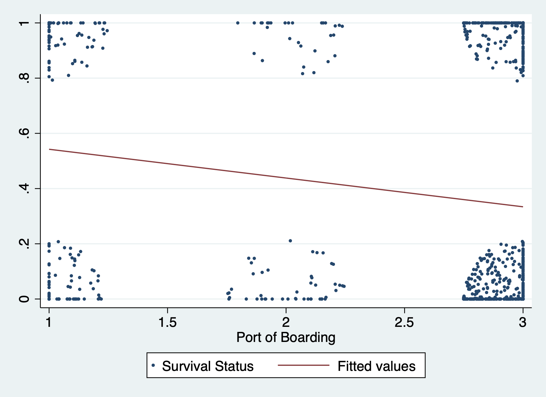
Plot your predicted probabilities in a margins plot
We will have a lab dedicated to reviewing margins plots, but for now here are a couple simple margins plots for this regression. With a normal linear regression, these plots display the predicted values of our outcome across different values of a covariate (or covariates). With a LPM the plots display the predicted probability of our outcome occurring across different values of a covariate (or covariates) we specify.
Predicted probability of surviving by boarding port
margins port
marginsplot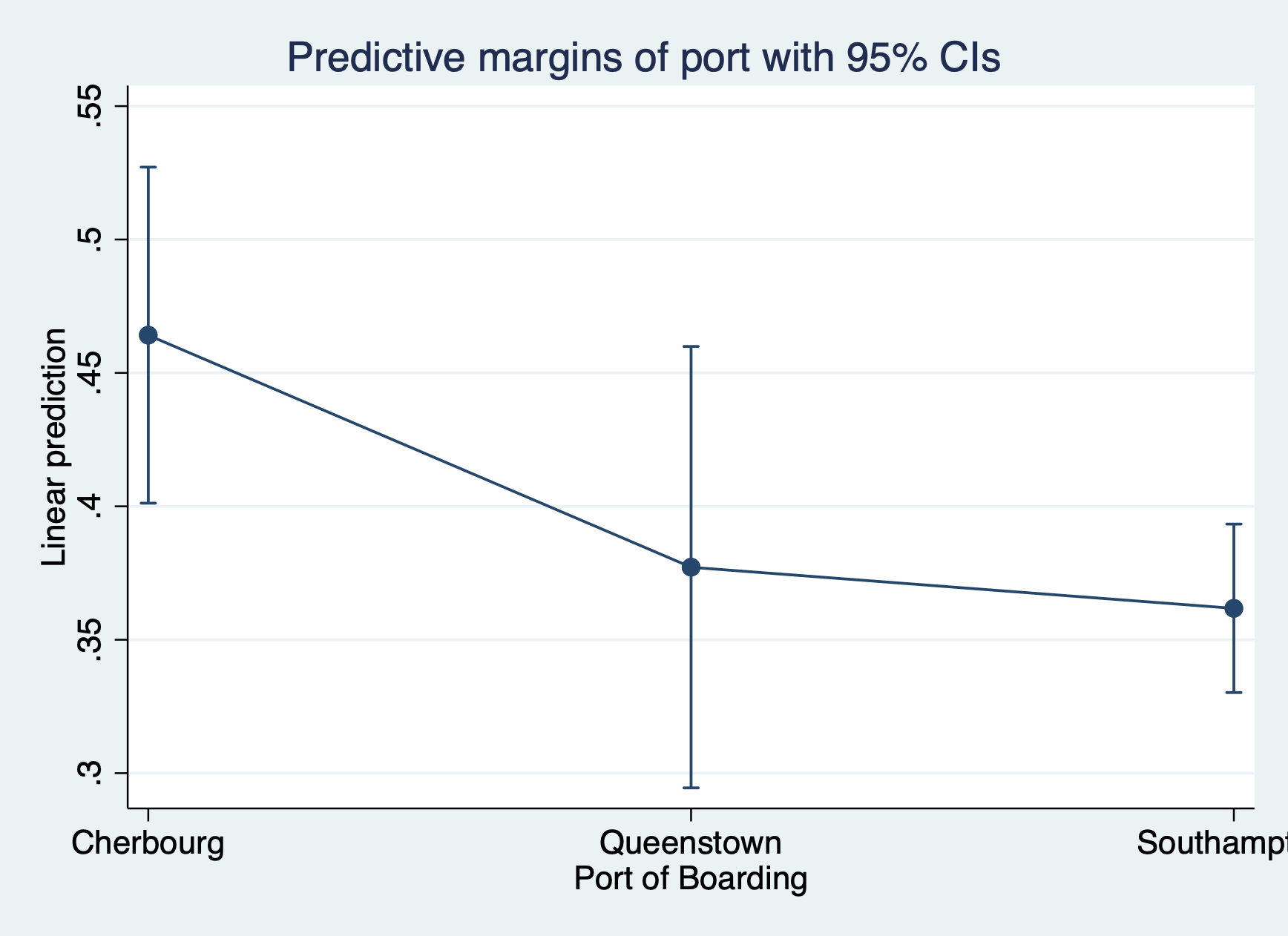
Predicted probability of surviving by boarding port by gender
margins port
marginsplot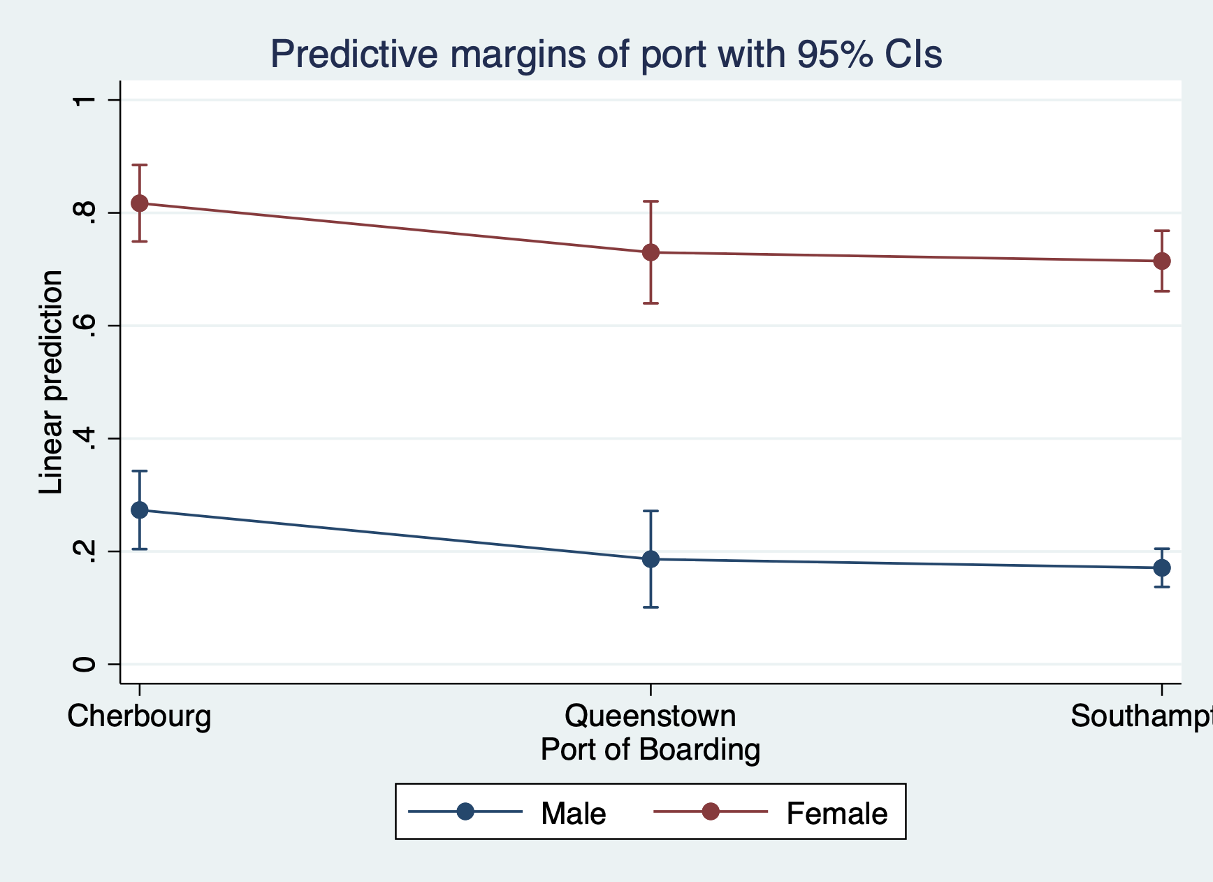
Step 4: Check your assumptions
1) Linearity assumption – violated!
But we don’t care so let’s move on.
2) Check out the violation of the heteroskedasticity assumption
We know we’re violating this assumption, but because you’ll be using this plot moving forward, let’s check out that violation with a…
Residuals vs Fitted Values Plot
rvfplot, yline(0)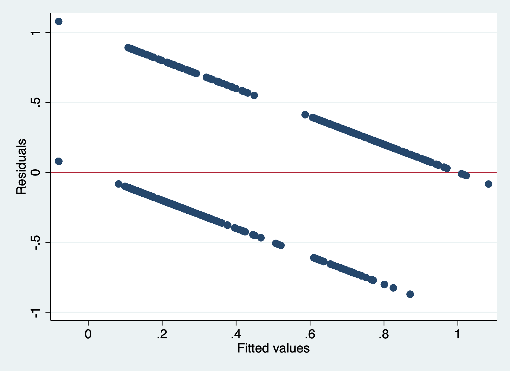
3) Normally distributed errors
To test this assumption you need to predict your residuals (or errors), which saves them as a new variable in your dataset that you can plot.
Predict your errors
predict r1 Then we’ll look at two plots, first a histogram…
hist r1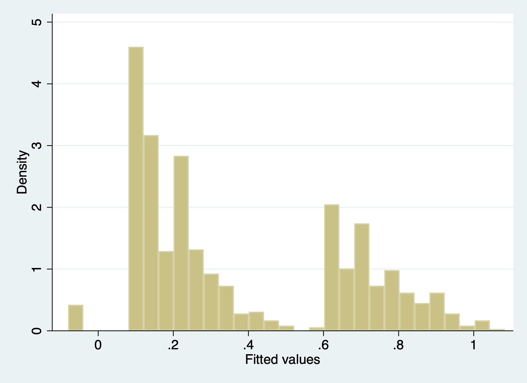
Not very normal at all!
And then we’ll look at the q-q plot. Remember, if the errors are normal they will stick close to the plotted line.
qnorm r1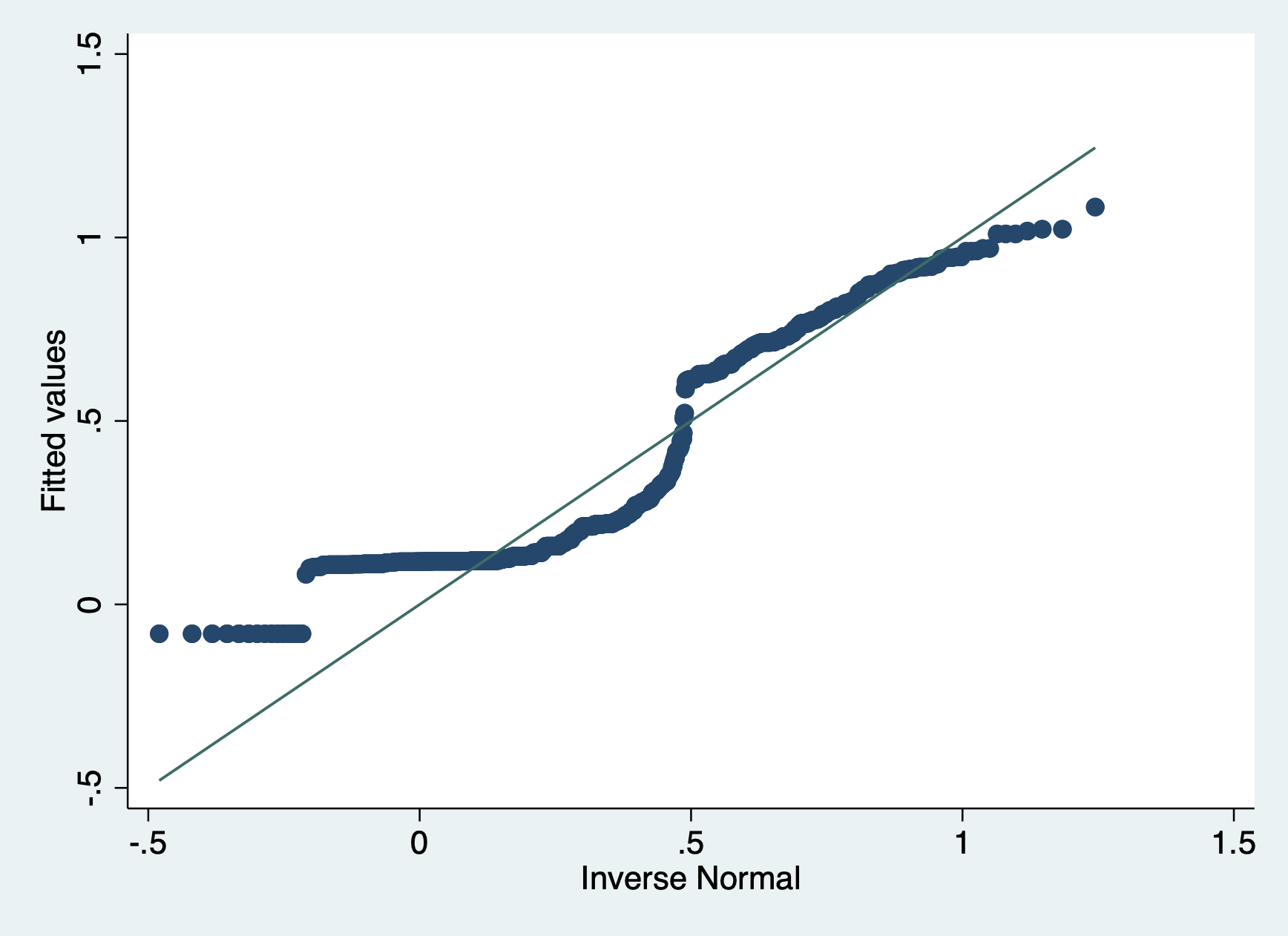
Also not normal!
We violate this assumption, but our sample size is high enough that we are okay.
5) X is not invariant
Logic check - yup, our x variables take on more than one value!
6) X is independent of the error term
Are there any confounding variables? For sure. Do we think they are a big enough detail that they would change our results.
We did not include passenger class, which if you know the story of the titanic had a huge effect on who lived and who died. This leads you to our application question…
2.4 Apply this model on your own
At the end of the .do file for this lab, run a LPM adding in passenger class (pclass) as an additional covariate.
- Interpret the
pclasscoefficient. - How does including this variable affect our other coefficients?
- (If time) Try to produce a margins plot for this variable.
Answers to these questions can be found in the “w.answers” version of the script file.