12 Handling Influential Observations (Stata)
12.1 Lab Overview
This is part 2 of lab 5, looking at how to handle influential observations in logistic regression.
Research Question: What characteristics are associated with separtist movements in ethnocultural groups?
Lab Files
Data:
Download M.A.R_Cleaned.dta
Codebook: Download MAR_Codebook.pdf
Script File: Download lab5_InfluentialObvs.do
12.2 DBETA
When looking for influential observations in logistic regressions, we use Pregibon’s dbeta to find the average change across all coefficients when that observation is removed.
Pregibon’s dbeta: Pregibon’s dbeta is a measure of how much influence an observation has on your model. It is very similar to Cook’s Distance (see the R lab), except it is less computationally intensive. It is a score that tells you how much the coefficients were changed if the observation at hand were removed. Higher means more influence. It calculates the score by computing the standardized differences in coefficients (aka betas) when an observation is removed.
NOTE: This will not work for probit regression. Stata does not have any built in options to find influential observations in probit regression.
There is no clear cut-off for a dbeta value that is “too high,” so visualizing dbeta over the predicted probability is important to helping you see what is a high influential observation.
Here is the typical process a person might undergo to evaluate their model.
STEP 1: Run regression, calculate dbeta
The first step is to run the logistic regression and generate the dbetas and the predicted probabilities for all observations. I am also going to label them to assist with our analysis.
logit sepkin i.trsntlkin kinmatsup kinmilsup i.grplang c.pct_ctry, nolog
    eststo est1

predict dbeta, dbeta
label variable dbeta "Pregibon Delta Beta"

predict phat, p
label variable phat "Predicted Probability"
Logistic regression Number of obs = 837
LR chi2(8) = 86.99
Prob > chi2 = 0.0000
Log likelihood = -463.4036 Pseudo R2 = 0.0858
-----------------------------------------------------------------------------------------------------
sepkin | Coefficient Std. err. z P>|z| [95% conf. interval]
------------------------------------+----------------------------------------------------------------
trsntlkin |
Close Kindred/Not Adjoining Base | 1.855838 .4394358 4.22 0.000 .9945597 2.717116
Close Kindred, Adjoining Base | 1.64484 .4544549 3.62 0.000 .7541243 2.535555
Close Kindred, More than 1 Country | 2.430812 .4495432 5.41 0.000 1.549723 3.3119
|
kinmatsup | -.2695913 .383968 -0.70 0.483 -1.022155 .4829722
kinmilsup | 1.546308 .4640465 3.33 0.001 .6367938 2.455822
|
grplang |
Some Speak Native Lang | .2350164 .2380003 0.99 0.323 -.2314556 .7014885
Most Speak Native Lang | 1.02658 .2753858 3.73 0.000 .4868337 1.566326
|
pct_ctry | -.0002825 .0061351 -0.05 0.963 -.012307 .0117421
_cons | -3.058763 .4824376 -6.34 0.000 -4.004323 -2.113203
-----------------------------------------------------------------------------------------------------
(15 missing values generated)
(15 missing values generated)STEP 2: Visualize dbeta over predicted probabilities
Create a scatter graph to see which variables are highly influential. Look for any observations that stand out. We add the unique id variable in the mlab() command to label the points.
scatter dbeta phat, mlab(numcode) 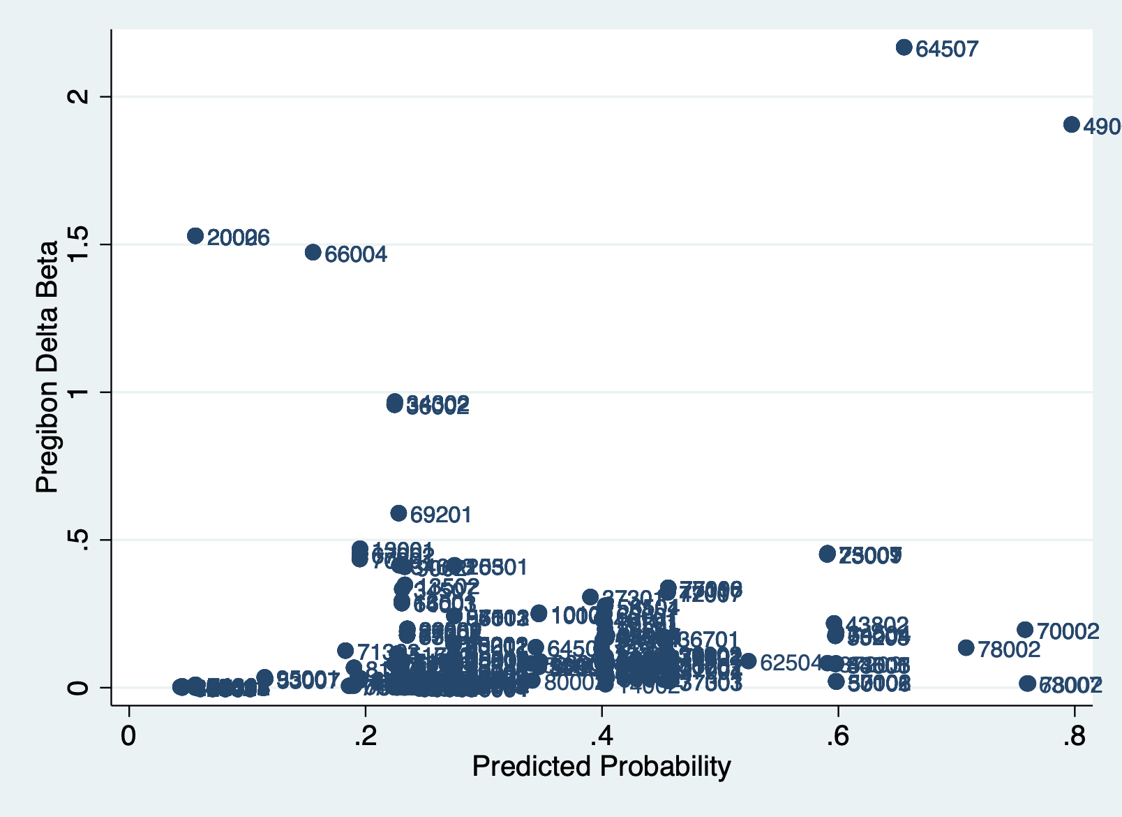
There really is no cutoff standard. To my eye, you could make arguments for cutoffs of .5, 1, or even 1.5. Lets look at what happens if we use .5 as the cutoff.
STEP 3: List the outliers
It’s always important to look holistically at the observations that are influential outliers according to dbeta. Think through why they might be different than the other observations, if they are important part of the pattern, or if different from the rest of the sample in some key way. Is there a theoretically difference why they might be different? Are the values wrong in some way? These aren’t questions with easy answers, but ones you need to think through as you decide what to include or exclude.
list numcode trsntlkin dbeta if dbeta > 0.5 & dbeta != . | numcode trsntlkin dbeta |
|---------------------------------------------------------|
16. | 2002 No Close Kindred 1.52948 |
17. | 2002 No Close Kindred 1.52948 |
18. | 2002 No Close Kindred 1.52948 |
130. | 20006 No Close Kindred 1.52954 |
131. | 20006 No Close Kindred 1.52954 |
|---------------------------------------------------------|
132. | 20006 No Close Kindred 1.52954 |
193. | 34302 Close Kindred/Not Adjoining Base .9684139 |
194. | 34302 Close Kindred/Not Adjoining Base .9684139 |
195. | 34302 Close Kindred/Not Adjoining Base .9684139 |
247. | 36002 Close Kindred/Not Adjoining Base .9575255 |
|---------------------------------------------------------|
248. | 36002 Close Kindred/Not Adjoining Base .9575255 |
249. | 36002 Close Kindred/Not Adjoining Base .9575255 |
424. | 49009 Close Kindred/Not Adjoining Base 1.906184 |
425. | 49009 Close Kindred/Not Adjoining Base 1.906184 |
426. | 49009 Close Kindred/Not Adjoining Base 1.906184 |
|---------------------------------------------------------|
601. | 64507 Close Kindred, More than 1 Country 2.16777 |
602. | 64507 Close Kindred, More than 1 Country 2.16777 |
603. | 64507 Close Kindred, More than 1 Country 2.16777 |
622. | 66004 Close Kindred, Adjoining Base 1.473813 |
623. | 66004 Close Kindred, Adjoining Base 1.473813 |
|---------------------------------------------------------|
624. | 66004 Close Kindred, Adjoining Base 1.473813 |
640. | 69201 Close Kindred/Not Adjoining Base .5906782 |
641. | 69201 Close Kindred/Not Adjoining Base .5906782 |
642. | 69201 Close Kindred/Not Adjoining Base .5906782 |
+---------------------------------------------------------+STEP 4: Run regression excluding potential influential observations
Once you do a visual scan and decide what your threshold will be, run a regression excluding observations above your selected dbeta.
logit sepkin i.trsntlkin kinmatsup kinmilsup i.grplang c.pct_ctry ///
        if dbeta < 0.5, nolog
eststo est2
> if dbeta < 0.5, nolog
note: 0.trsntlkin != 0 predicts failure perfectly;
0.trsntlkin omitted and 99 obs not used.
note: 3.trsntlkin omitted because of collinearity.
Logistic regression Number of obs = 714
LR chi2(7) = 85.32
Prob > chi2 = 0.0000
Log likelihood = -404.56366 Pseudo R2 = 0.0954
-----------------------------------------------------------------------------------------------------
sepkin | Coefficient Std. err. z P>|z| [95% conf. interval]
------------------------------------+----------------------------------------------------------------
trsntlkin |
No Close Kindred | 0 (empty)
Close Kindred/Not Adjoining Base | -.6523045 .2072025 -3.15 0.002 -1.058414 -.246195
Close Kindred, Adjoining Base | -1.004568 .2411389 -4.17 0.000 -1.477192 -.5319447
Close Kindred, More than 1 Country | 0 (omitted)
|
kinmatsup | -2.329287 .8737652 -2.67 0.008 -4.041836 -.6167388
kinmilsup | 3.781221 .8897452 4.25 0.000 2.037352 5.52509
|
grplang |
Some Speak Native Lang | .1692215 .2551201 0.66 0.507 -.3308048 .6692477
Most Speak Native Lang | 1.194825 .2917816 4.09 0.000 .6229435 1.766706
|
pct_ctry | -.0032303 .0069341 -0.47 0.641 -.016821 .0103603
_cons | -.5358927 .3103325 -1.73 0.084 -1.144133 .0723478
-----------------------------------------------------------------------------------------------------Then create a table to compare how the coefficients changed. Note I stored the results from the first regressuion using estab.
esttab est1 est2 (1) (2)
sepkin sepkin
--------------------------------------------
sepkin
0.trsntlkin 0 0
(.) (.)
1.trsntlkin 1.856*** -0.652**
(4.22) (-3.15)
2.trsntlkin 1.645*** -1.005***
(3.62) (-4.17)
3.trsntlkin 2.431*** 0
(5.41) (.)
kinmatsup -0.270 -2.329**
(-0.70) (-2.67)
kinmilsup 1.546*** 3.781***
(3.33) (4.25)
0.grplang 0 0
(.) (.)
1.grplang 0.235 0.169
(0.99) (0.66)
2.grplang 1.027*** 1.195***
(3.73) (4.09)
pct_ctry -0.000282 -0.00323
(-0.05) (-0.47)
_cons -3.059*** -0.536
(-6.34) (-1.73)
--------------------------------------------
N 837 714
--------------------------------------------
t statistics in parentheses
* p<0.05, ** p<0.01, *** p<0.001There are some pretty significant differences!
At the end of the day there is no hard and fast rule about what influential observations to exclude. You can use these processes to identify variables that are outliers and statistically influential, but then it’s up to you to examine each potential outlier and decide according to your theory and knowledge of the data whether it makes sense to exclude them from your analysis. Ask yourself: “If I include this/these observation(s) will my data be telling an incorrect story?”