14 Multinomial Logit Regression (Stata)
14.1 Lab Overview
This web page provides a brief overview of multinomial logit regression and a detailed explanation of how to run this type of regression in Stata. Download the script file to execute sample code for logit regression regression. We’re using the same ethnocultural groups (MAR) dataset.
Research Question: What characteristics are associated with the types of cultural grievances expressed by ethnocultural groups at risk?
Lab Files
Data:
Download M.A.R_Cleaned.dta
Script File: Download lab6_MLR.do
14.2 Multinomial Logit Regression Review
Multionmial logistic regression extends the model we use for typical binary logistic regression to a categorical outcome variable with more than two categories. Like our past regressions, the most complicated part of multinomial logistic regression is the interpretation. However, our interpretation is more complex than any of the previous models. We’ll walk through a brief overview of the model carefully to try to build more intuition when running this type of regression.
Overall, I want you to think of multinomial logistic regression as stacking two or more logistic regressions on top of each other.
The Equation
If you recall, our logistic regression equation is as follows:
\[\ln(\displaystyle \frac{P}{1-P}) = \beta_0 + \beta_1X_1 + ... \beta_kX_k\]
We use the logistic equation as the link function, which transforms our outcome into log-odds.
For multinomial logistic regression, our outcome, instead of being the log odds, becomes the log odds of the probability of one category over the probability of the base category. Let’s say category A is the base category. I am going to refer to probability as \(P\). Our outcome is now the natural log of this ratio (still log-odds, just with a ratio now). This is called the relative log-odds:
\[\ln(\displaystyle \frac{P_{categoryB}}{P_{categoryA}})\]
So if we had three categories in our outcome: Category A, Category B, and Category C. We decide that Category A is our base category, and then we have two equations: one for Category B and one for Category C.
Equation 1: Category B compared to Category A \[\ln(\displaystyle \frac{P_{categoryB}}{P_{categoryA}}) = \beta_0 + \beta_1X_1 + ... \beta_kX_k\] Equation 2: Category C compared to Category A \[\ln(\displaystyle \frac{P_{categoryC}}{P_{categoryA}}) = \beta_0 + \beta_1X_1 + ... \beta_kX_k\] So what’s the takeaway?
- We have two equations that each run as a binary regression.
- The first equation looks to see how a one unit change in each coefficient changes the log-odds of going from Category A to Category B.
- The second equation looks to see how a one unit change in each coefficient changes the log-odds of going from Category C to Category B.
- Again, it’s like we’re stacking two binary regressions on top of each other.
Big Point: Because every coefficient in this model refers back to the base category, you need to think carefully through which reference category to choose. This is not a statistics question, it is a theoretical/knowledge question. You have to think what set of comparison is the most interesting or relevant.
The Interpretation
We have four options for interpreting coefficients in multinomial logistic regression. They are pretty much the same as logistic regression, just formatted as a comparison from the base category to another category.
- Relative Log Odds: This is equivalent to log-odds in the logistic regression. This is the default output in Stata.
“A one-unit change in X is associated with a [blank] change in the log odds of being in category B compared to the base category.”
- Relative Risk Ratios: This is equivalent to odds ratios in logistic regression. It’s calculated by exponentiating the coefficient (\(e^\beta\)). It is very common to refer to odds here as “risk,” but they are interchangeable.
“A one-unit change in X is associated with a [blank] change in the”risk" of being in category B compared to the base category."
- Predicted Probabilities: The same thing as logistic regression, but it’s the probability of falling in a specific category. Stata will calculate this for you using the margins command you should be familiar with. Again, Stata is plugging in values for the covarites into the equation, and calculating a predicted value in terms of the probability of the outcome (or in this case being in a given category).
“An observation with these values has a [blank] predicted probability of being in [blank] category.”
Note: We no longer have to reference the base category for the outcome. Stata will produce a predicted probability for being in each category in our analysis, BUT if your independent variable is categorical it won’t produce predicted probabilities for the base category for that variable.
- Marginal Effects: The same thing as logistic regression, but it’s the change in probability of falling into a specific category. Stata will calculate this for you using the margins command you should be familiar with and the
dydx()option.
“A one unit change in X is associated with a [blank] change in the probability of being in [blank] category.”
Note: Here we also no longer have to reference the base category. Stata will produce a marginal effect for the probability of being in each category in our analysis. BUT if your independent variable is categorical it won’t produce predicted probabilities for the base category for that variable.
The Output
I am adding this category because making sense of the output in Stata can be difficult for multinomial logistic regressions. It’s the sorting through of all the results that you will have to work through carefully. We’ll go through the interpretation of this model more below when we get to the practical example in Stata. This is to help you know what to expect when you run a multinomial logistic regression in Stata.
What you should look for in the output:
- No base category coefficients: You will see an empty line where the name of your base category is listed. All the coefficients will be in relative log-odds or relative risk ratios comparing back to this category.
- Second Category: The second chunk in the output will be the coefficients for the second category. Remember, all these coefficients are like a binary logistic regression telling you the relative log-odds or relative risk of being in category 2 compared to the base category.
- Third Category: Next comes the third chunk with all the coefficients for the third category. Same deal as the second chunk, all these coefficients are like a binary logistic regression telling you the relative log-odds or relative risk of being in category 3 compared to the base category.
The Assumptions
These assumptions are pretty much the same as logistic regression with the addition of one big one, which we’ll cover first.
(1) Independence of irrelevant alternatives (IIA)
This assumption states that the relative likelihood of being in one category compared to the base category would not change if you added any other categories. Remember that multinomial logistic regression almost stacks two logistic regressions in one model. This assumption extends from that and the relative independence of those two stacked regressions. The likelihood of being in category B compared to base category A should not change whether or not category C is an option.
Here’s a practical example offered by Benson(2016): A man asks his date if she wants to go to a rock concert or a classical music concert. She chooses classical music, but when he adds that jazz is also an option she says she’d actually like jazz the best. Jazz is a relevant alternative and would violate the IIA assumption.
Remember this is particularly important if two of the options are relatively similar and another option is quite different. The relative similarity of options A and B obscure the big difference between options A and C.
How to address it?
There are not good statistical tests to address this problem, so you are going to have to rely on your knowledge of the variables in the dataset. You have to make a judgment call whether you think two categories are too similar and try your best to make each category is a unique option.
(2) The outcome is categorical
A categorical variable appropriate for multinomial logistic regression has three or more possible response categories. Technically you can run this model for ordered or unordered categorical variables, but other models are recommended for ordinal outcome variables.
(3) The log-odds of the outcome and independent variable have a linear relationship
Like normal logistic regression, the log-odds of the outcome vs the any continuous explanatory variables should have a linear relationship.
How to address it?
Like a linear regression, you can play around with squared and cubed terms to see if they address the curved relationship in your data.
(4) Errors are independent
Like linear regression we don’t want to have obvious clusters in our data. Examples of clusters would be multiple observations from the same person at different times, multiple observations withing schools, people within cities, and so on.
How to address it?
If you have a variable identifying the cluster (e.g., year, school, city, person), you can run a logistic regression adjusted for clustering using cluster-robust standard errors (rule of thumb is to have 50 clusters for this method). However, you may also want to consider learning about and applying a hierarchical linear model.
(5) No severe multicolinearity
This is another carryover from linear regression. Multicollineary can throw a wrench in your model when one or more independent variables are correlated to one another.
How to address it?
Run a VIF (variance inflation factor) to detect correlation between your independent variables. Consider dropping variables or combining them into one factor variable.
The Pros and Cons
Pros:
- The basic interpretation is very similar to a binary logistic regression.
- Logistic regression are the most common model used for categorical outcomes.
Cons:
- The many coefficients can be complicated to interpret and lead to complex results.
- It assumes linearity between log-odds outcome and continuous explanatory variables.
14.3 Running a MLR in Stata
Now we will walk through running and interpreting a multinomial logistic regression in Stata from start to finish. To run the regression we’ll be using the mlogit command.
These steps assume that you have already:
- Cleaned your data.
- Run descriptive statistics to get to know your data in and out.
- Transformed variables that need to be transformed (logged, squared, etc.)
We will be running a multinomial logistic regression to see what characteristics are associated with the types of cultural grievances expressed by ethnocultural groups at risk. We will use the variable ‘culgrieve’ as our outcome, which represents the level of cultural grievances expressed by ethnic groups at risk. This variable has three values (the outcomes for our multinomial):
0 - No Grievances Expressed
1 - Ending Discrmination
2 - Creating/Strengthening Remedial Policies
STEP 1: Plot your outcome and key independent variable
We’ll plot two plots instead of one in order to look at our two stacked regressions separately.
Category 0 compared to Category 1
scatter culgrieve grplang if culgrieve == 0 | culgrieve == 1 || ///
lowess culgrieve grplang if culgrieve == 0 | culgrieve == 1 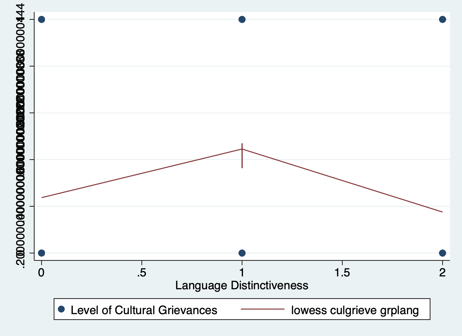
Category 0 compared to Category 2
scatter culgrieve grplang if culgrieve == 0 | culgrieve == 2 || ///
lowess culgrieve grplang if culgrieve == 0 | culgrieve == 2 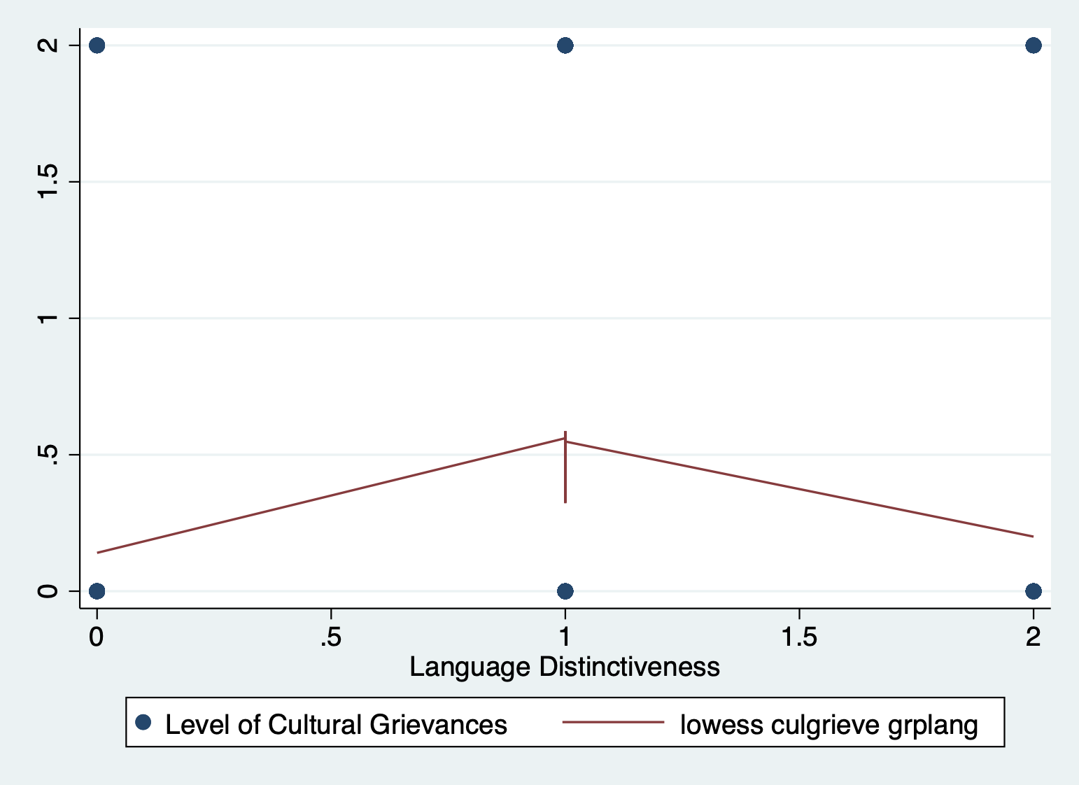
STEP 2: Run your models
Running a multinomial logit command in Stata is not too difficult. The syntax of the command is the same as other regressions just with mlogit.
First run a basic model with your outcome and key independent variable. The nolog option is added just to condense the output.
mlogit culgrieve i.grplang, nologMultinomial logistic regression Number of obs = 848
LR chi2(4) = 66.11
Prob > chi2 = 0.0000
Log likelihood = -775.91756 Pseudo R2 = 0.0409
-------------------------------------------------------------------------------------------------
culgrieve | Coefficient Std. err. z P>|z| [95% conf. interval]
--------------------------------+----------------------------------------------------------------
No_Grievances_Expressed | (base outcome)
--------------------------------+----------------------------------------------------------------
Ending_Discrimination |
grplang |
Some Speak Native Lang | .9490701 .2108233 4.50 0.000 .535864 1.362276
Most Speak Native Lang | -.3784314 .2969308 -1.27 0.202 -.9604051 .2035423
|
_cons | -1.168206 .1882296 -6.21 0.000 -1.537129 -.7992823
--------------------------------+----------------------------------------------------------------
Creating_Strengthening_Remedial |
grplang |
Some Speak Native Lang | 1.575306 .3667691 4.30 0.000 .8564514 2.29416
Most Speak Native Lang | .3846743 .4605508 0.84 0.404 -.5179887 1.287337
|
_cons | -2.581899 .3457087 -7.47 0.000 -3.259475 -1.904322
-------------------------------------------------------------------------------------------------Then add in your other covariates.
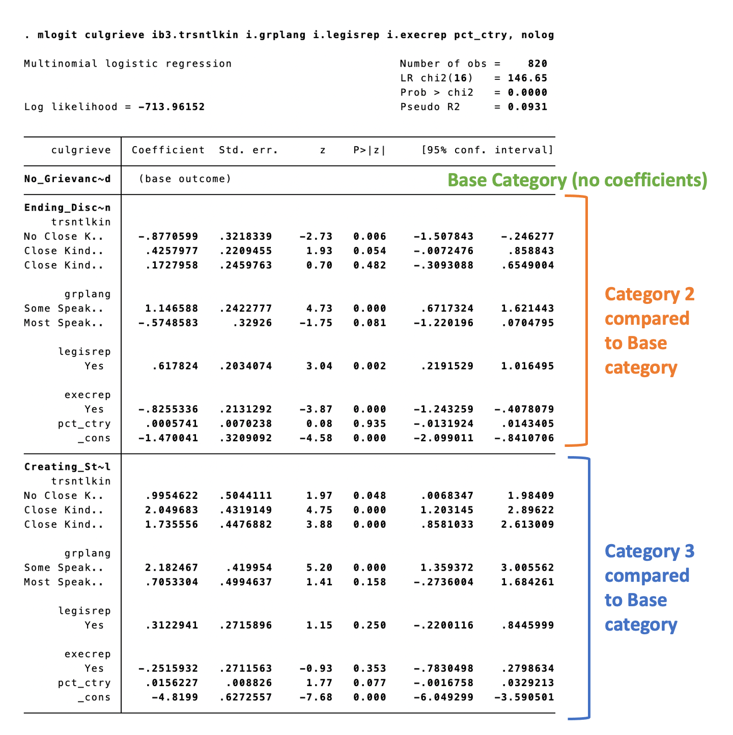
mlogit culgrieve i.grplang i.trsntlkin i.legisrep i.execrep pct_ctry, nologMultinomial logistic regression Number of obs = 820
LR chi2(16) = 146.65
Prob > chi2 = 0.0000
Log likelihood = -713.96152 Pseudo R2 = 0.0931
-----------------------------------------------------------------------------------------------------
culgrieve | Coefficient Std. err. z P>|z| [95% conf. interval]
------------------------------------+----------------------------------------------------------------
No_Grievances_Expressed | (base outcome)
------------------------------------+----------------------------------------------------------------
Ending_Discrimination |
grplang |
Some Speak Native Lang | 1.146588 .2422777 4.73 0.000 .6717324 1.621443
Most Speak Native Lang | -.5748583 .32926 -1.75 0.081 -1.220196 .0704795
|
trsntlkin |
Close Kindred/Not Adjoining Base | 1.302858 .3015785 4.32 0.000 .7117746 1.893941
Close Kindred, Adjoining Base | 1.049856 .3204527 3.28 0.001 .42178 1.677931
Close Kindred, More than 1 Country | .8770599 .3218339 2.73 0.006 .246277 1.507843
|
legisrep |
Yes | .617824 .2034074 3.04 0.002 .2191529 1.016495
|
execrep |
Yes | -.8255336 .2131292 -3.87 0.000 -1.243259 -.4078079
pct_ctry | .0005741 .0070238 0.08 0.935 -.0131924 .0143405
_cons | -2.347101 .3775301 -6.22 0.000 -3.087046 -1.607155
------------------------------------+----------------------------------------------------------------
Creating_Strengthening_Remedial |
grplang |
Some Speak Native Lang | 2.182467 .419954 5.20 0.000 1.359372 3.005562
Most Speak Native Lang | .7053304 .4994637 1.41 0.158 -.2736004 1.684261
|
trsntlkin |
Close Kindred/Not Adjoining Base | 1.05422 .353805 2.98 0.003 .3607755 1.747665
Close Kindred, Adjoining Base | .7400939 .3750042 1.97 0.048 .0050992 1.475089
Close Kindred, More than 1 Country | -.9954622 .5044111 -1.97 0.048 -1.98409 -.0068347
|
legisrep |
Yes | .3122941 .2715896 1.15 0.250 -.2200116 .8445999
|
execrep |
Yes | -.2515932 .2711563 -0.93 0.353 -.7830498 .2798634
pct_ctry | .0156227 .008826 1.77 0.077 -.0016758 .0329213
_cons | -3.824438 .5650666 -6.77 0.000 -4.931948 -2.716928
-----------------------------------------------------------------------------------------------------And finally, run the full model and add rrr to exponentiate the coefficients and get the relative risk ratios.
mlogit culgrieve i.grplang i.trsntlkin i.legisrep i.execrep pct_ctry, rrr nologMultinomial logistic regression Number of obs = 820
LR chi2(16) = 146.65
Prob > chi2 = 0.0000
Log likelihood = -713.96152 Pseudo R2 = 0.0931
-----------------------------------------------------------------------------------------------------
culgrieve | RRR Std. err. z P>|z| [95% conf. interval]
------------------------------------+----------------------------------------------------------------
No_Grievances_Expressed | (base outcome)
------------------------------------+----------------------------------------------------------------
Ending_Discrimination |
grplang |
Some Speak Native Lang | 3.147435 .7625533 4.73 0.000 1.957626 5.060389
Most Speak Native Lang | .5627846 .1853025 -1.75 0.081 .2951723 1.073023
|
trsntlkin |
Close Kindred/Not Adjoining Base | 3.679797 1.109748 4.32 0.000 2.037604 6.645505
Close Kindred, Adjoining Base | 2.857239 .9156098 3.28 0.001 1.524673 5.354468
Close Kindred, More than 1 Country | 2.403822 .7736315 2.73 0.006 1.279254 4.516976
|
legisrep |
Yes | 1.854887 .3772978 3.04 0.002 1.245022 2.763492
|
execrep |
Yes | .4380012 .0933509 -3.87 0.000 .2884426 .6651066
pct_ctry | 1.000574 .0070279 0.08 0.935 .9868943 1.014444
_cons | .0956461 .0361093 -6.22 0.000 .0456366 .200457
------------------------------------+----------------------------------------------------------------
Creating_Strengthening_Remedial |
grplang |
Some Speak Native Lang | 8.868158 3.724218 5.20 0.000 3.893749 20.19756
Most Speak Native Lang | 2.024516 1.011172 1.41 0.158 .760636 5.388469
|
trsntlkin |
Close Kindred/Not Adjoining Base | 2.869737 1.015327 2.98 0.003 1.434441 5.741184
Close Kindred, Adjoining Base | 2.096132 .7860584 1.97 0.048 1.005112 4.371423
Close Kindred, More than 1 Country | .3695526 .1864064 -1.97 0.048 .1375057 .9931886
|
legisrep |
Yes | 1.366557 .3711425 1.15 0.250 .8025095 2.327047
|
execrep |
Yes | .777561 .2108406 -0.93 0.353 .4570101 1.322949
pct_ctry | 1.015745 .0089649 1.77 0.077 .9983256 1.033469
_cons | .0218307 .0123358 -6.77 0.000 .0072124 .0660775
-----------------------------------------------------------------------------------------------------
Note: _cons estimates baseline relative risk for each outcome.STEP 3: Interpret your model
Interpretation is the hard part. We’ll practice in the lab together. For each of our four ways to interpret the model, I will interpret the coefficients for one continuous variable (pct_ctry) and one categorical variable (grplang).
Relative Log-Odds
Percent of population:
- Category: Ending Discrimination
- A one unit increase in percent population is associated with a .0006 increase in the log-odds of an ethnocultural group wanting to end discrimination vs having no grievances. It is not statistically significant.
- Category: Creating/Strengthening Remedial Policies
- A one unit increase in percent population is associated with a .0156 increase in the log-odds of an ethnocultural group wanting to create or strengthen remedial policies vs having no cultural grievances. It is not statistically significant.
Language distinctiveness:
- Category: Ending Discrimination
- A group where some medium percentage of members speak the native language (compared to groups where <10% speak the language) is associated with a 1.147 increase in the log-odds of a group wanting to end discrimination compared to having no cultural grievances.
- A group where most members speak the native language (compared to groups where <10% speak the language) is associated with a .575 decrease in the log-odds of a group wanting to end discrimination compared to having no cultural grievances. It is not statistically significant.
- Category: Creating/Strengthening Remedial Policies
- A group where some medium percentage of members speak the native language (compared to groups where <10% speak the language) is associated with a 2.182 increase in the log-odds of a group wanting to create/strengthen remedial policies compared to having no cultural grievances.
- A group where most members speak the native language (compared to groups where <10% speak the language) is associated with a .705 decrease in the log-odds of a group wanting to create/strengthen remedial policies compared to having no cultural grievances. It is not statistically significant.
Relative Risk Ratios
Percent of population:
- Category: Ending Discrimination
- A one unit increase in percent population multiplies the odds of wanting to end discrimination vs having no grievances by 1.0006 (basically 0%). It is not statistically significant.
- Category: Creating/Strengthening Remedial Policies
- A one unit increase in percent population multiplies the odds of wanting to create or strengthen remedial policies vs having no cultural grievances by 1.016 (1.6%). It is not statistically signifcant.
Language distinctiveness:
- Category: Ending Discrimination
- A group where some medium percentage of members speak the native language (compared to groups where <10% speak the language) is multiplies the odds of wanting to end discrimination compared to having no cultural grievances by 3.15 (215%).
- A group where most members speak the native language (compared to groups where <10% speak the language) multiplies the odds of wanting to end discrimination compared to having no cultural grievances by .562 (-43.8%). It is not statistically significant.
- Category: Creating/Strengthening Remedial Policies
- A group where some medium percentage of members speak the native language (compared to groups where <10% speak the language) multiplies the odds of wanting to create/strengthen remedial policies compared to having no cultural grievances by 8.87 (786.8 %).
- A group where most members speak the native language (compared to groups where <10% speak the language) multiplies the odds of wanting to create/strengthen remedial policies compared to having no cultural grievances by 2.02 (102%). It is not statistically significant.
Marginal Effects
Percent of population:
margins, dydx(pct_ctry)Average marginal effects Number of obs = 820
Model VCE: OIM
dy/dx wrt: pct_ctry
1._predict: Pr(culgrieve==No_Grievances_Expressed), predict(pr outcome(0))
2._predict: Pr(culgrieve==Ending_Discrimination), predict(pr outcome(1))
3._predict: Pr(culgrieve==Creating_Strengthening_Remedial), predict(pr outcome(2))
------------------------------------------------------------------------------
| Delta-method
| dy/dx std. err. z P>|z| [95% conf. interval]
-------------+----------------------------------------------------------------
pct_ctry |
_predict |
1 | -.0010959 .0013132 -0.83 0.404 -.0036698 .001478
2 | -.0006117 .001317 -0.46 0.642 -.003193 .0019697
3 | .0017075 .0009463 1.80 0.071 -.0001472 .0035622
------------------------------------------------------------------------------Category 1: No Grievances
- A one unit increase in the percent the group represents in the total population is associated with a .001 descrease in the probability that the group has no grievances.
Category 2: Ending Discrimination
- A one unit increase in the percent the group represents in the total population is associated with a .0006 decrease in the probability that the group wants to end discrimination.
Category 3: Creating/Strengthening Remedial Policies
- A one unit increase in the percent the group represents in the total population is associated with a .002 increase in the probability that the group wants to create or strengthen remedial policies.
Language Distinctiveness:
margins, dydx(grplang)Average marginal effects Number of obs = 820
Model VCE: OIM
dy/dx wrt: 1.grplang 2.grplang
1._predict: Pr(culgrieve==No_Grievances_Expressed), predict(pr outcome(0))
2._predict: Pr(culgrieve==Ending_Discrimination), predict(pr outcome(1))
3._predict: Pr(culgrieve==Creating_Strengthening_Remedial), predict(pr outcome(2))
------------------------------------------------------------------------------
| Delta-method
| dy/dx std. err. z P>|z| [95% conf. interval]
-------------+----------------------------------------------------------------
0.grplang | (base outcome)
-------------+----------------------------------------------------------------
1.grplang |
_predict |
1 | -.3072404 .0428567 -7.17 0.000 -.391238 -.2232428
2 | .1569385 .0414252 3.79 0.000 .0757466 .2381304
3 | .1503019 .0240357 6.25 0.000 .1031928 .197411
-------------+----------------------------------------------------------------
2.grplang |
_predict |
1 | .04122 .0498993 0.83 0.409 -.0565809 .1390209
2 | -.0870293 .0443172 -1.96 0.050 -.1738894 -.0001693
3 | .0458093 .0280464 1.63 0.102 -.0091606 .1007792
------------------------------------------------------------------------------
Note: dy/dx for factor levels is the discrete change from the base level.Category 1: No Grievances
- A group where some medium percentage of members speak the native language (compared to groups where <10% speak the language) is associated with a .307 decrease in the probability of having no grievances.
- A group where most members speak the native language (compared to groups where <10% speak the language) is associated with a .041 increase in the probability of having no grievances. It is not statistically significant.
Category 2: Ending Discrimination
- A group where some medium percentage of members speak the native language (compared to groups where <10% speak the language) is associated with a .157 increase in the probability of wanting to end discrimination.
- A group where most members speak the native language (compared to groups where <10% speak the language) is associated with a .087 decrease in the probability of wanting to end discrimination. It is not statistically significant.
Category 3: Creating/Strengthening Remedial Policies
- A group where some medium percentage of members speak the native language (compared to groups where <10% speak the language) is associated with a .150 increase in the probability of wanting to create or strengthen remedial policies.
- A group where most members speak the native language (compared to groups where <10% speak the language) is associated with a .045 increase in the probability of wanting to create/strengthen remedial policies. It is not statistically significant.
Predicted Probabilities
Because in class you all pointed out the difficulties of reading these plots because of the formatting, I decided to format these using our shortcuts (go to the graph fundamentals lab for code to install).
Set the new default styles for your graph
grstyle clear
set scheme s2color
grstyle init
grstyle set plain, box
grstyle color background white
grstyle set color mono
grstyle set color Dark2, n(3)
grstyle yesno draw_major_hgrid yes
grstyle yesno draw_major_ygrid yes
grstyle set size 14pt: axis_title
Percent of Population
quietly margins, at(pct_ctry = (0(20)80)) atmeans
marginsplot, ///
    legend(order(1 "Ending Discrimination" ///
                 2 "Remedial Policies" ///
                 0 "No Grievances"))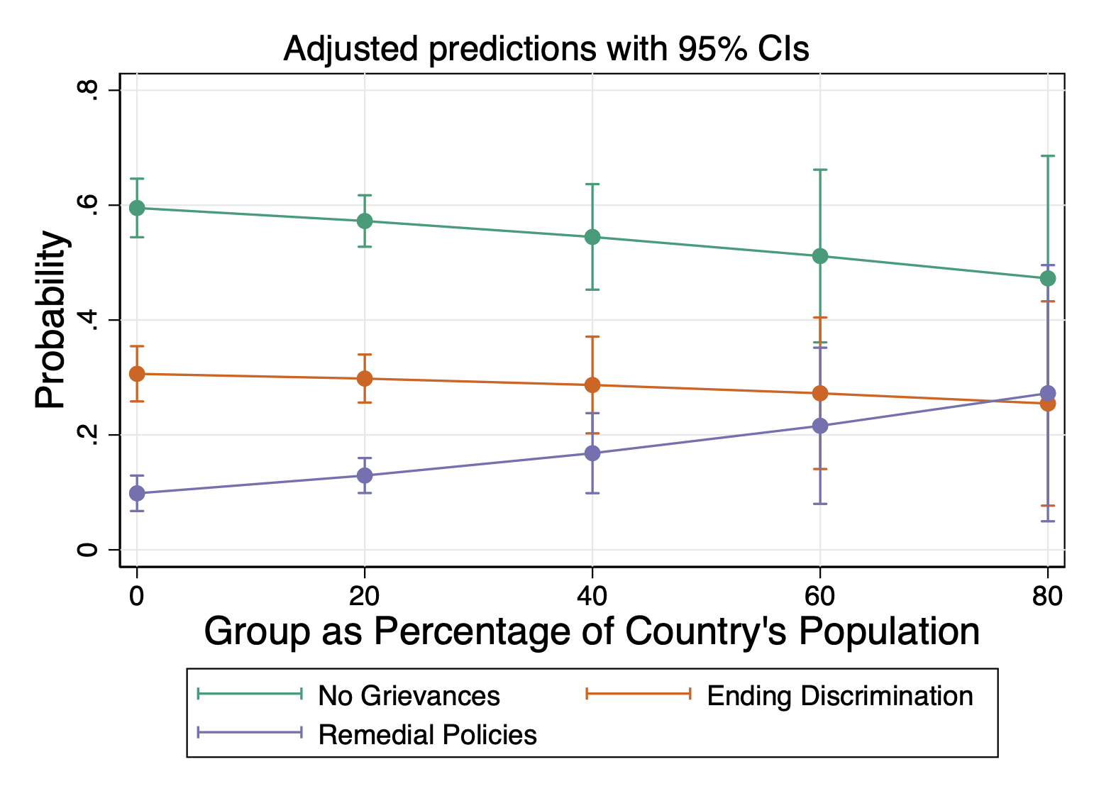
Language Distinctiveness
quietly margins grplang, atmeans
marginsplot, ///
    legend(order(1 "Ending Discrimination" ///
                 2 "Remedial Policies" ///
                 0 "No Grievances"))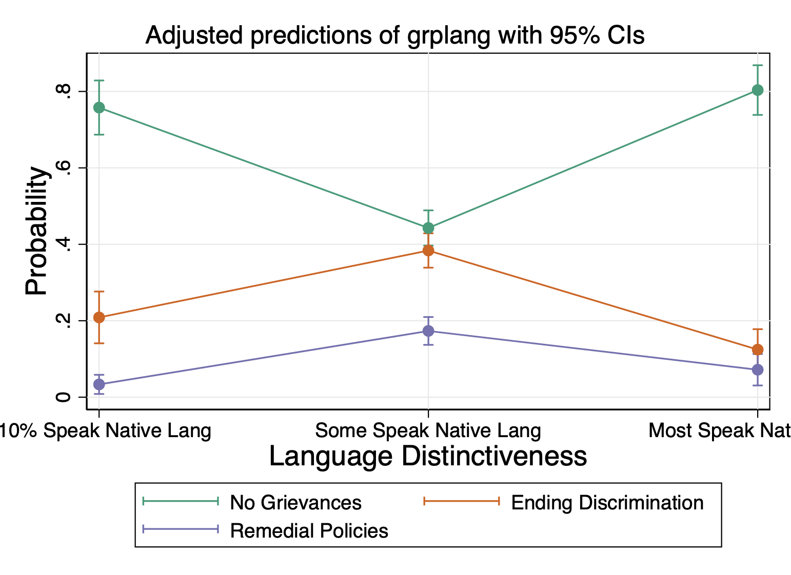
STEP 4: Check your assumptions
To keep this lab from being too long and because the way you check assumptions carries over from logistic regression, I am not going to include them in this lab.
But if we were checking for the independence of irrelevant alternatives (IIA) assumption, we would want to make sure that we were sure ending discrimination and remedial policies are truly distinct categories.
14.4 Wald Test for MLR
Overall, the Wald test is identical to what you would do for all the other models. The one thing that is different, however, is that the name of coefficients are a little different given multiple outcome categories. That is where ‘coeflegend’ comes in: it allows you to see the exact name of a variable so you can get its name right. Beyond this, we interpret the Wald test the same way we do in previous contexts.
quietly mlogit culgrieve ib3.trsntlkin i.grplang legisrep execrep pct_ctry, rrr
mlogit, coeflegend
Multinomial logistic regression Number of obs = 820
LR chi2(16) = 146.65
Prob > chi2 = 0.0000
Log likelihood = -713.96152 Pseudo R2 = 0.0931
---------------------------------------------------------------------------------------------------
culgrieve | Coefficient Legend
----------------------------------+----------------------------------------------------------------
No_Grievances_Expressed | (base outcome)
----------------------------------+----------------------------------------------------------------
Ending_Discrimination |
trsntlkin |
No Close Kindred | -.8770599 _b[Ending_Discrimination:0.trsntlkin]
Close Kindred/Not Adjoining Base | .4257977 _b[Ending_Discrimination:1.trsntlkin]
Close Kindred, Adjoining Base | .1727958 _b[Ending_Discrimination:2.trsntlkin]
|
grplang |
Some Speak Native Lang | 1.146588 _b[Ending_Discrimination:1.grplang]
Most Speak Native Lang | -.5748583 _b[Ending_Discrimination:2.grplang]
|
legisrep | .617824 _b[Ending_Discrimination:legisrep]
execrep | -.8255336 _b[Ending_Discrimination:execrep]
pct_ctry | .0005741 _b[Ending_Discrimination:pct_ctry]
_cons | -1.470041 _b[Ending_Discrimination:_cons]
----------------------------------+----------------------------------------------------------------
Creating_Strengthening_Remedial |
trsntlkin |
No Close Kindred | .9954622 _b[Creating_Strengthening_Remedial:0.trsntlkin]
Close Kindred/Not Adjoining Base | 2.049683 _b[Creating_Strengthening_Remedial:1.trsntlkin]
Close Kindred, Adjoining Base | 1.735556 _b[Creating_Strengthening_Remedial:2.trsntlkin]
|
grplang |
Some Speak Native Lang | 2.182467 _b[Creating_Strengthening_Remedial:1.grplang]
Most Speak Native Lang | .7053304 _b[Creating_Strengthening_Remedial:2.grplang]
|
legisrep | .3122941 _b[Creating_Strengthening_Remedial:legisrep]
execrep | -.2515932 _b[Creating_Strengthening_Remedial:execrep]
pct_ctry | .0156227 _b[Creating_Strengthening_Remedial:pct_ctry]
_cons | -4.8199 _b[Creating_Strengthening_Remedial:_cons]
---------------------------------------------------------------------------------------------------Test if adding pct_ctry has an effect for both outcomes
test (_b[Ending_Discrimination:pct_ctry] = 0 ) ///
    (_b[Creating_Strengthening_Remedial:pct_ctry] = 0 )
> (_b[Creating_Strengthening_Remedial:pct_ctry] = 0 )
( 1) [Ending_Discrimination]pct_ctry = 0
( 2) [Creating_Strengthening_Remedial]pct_ctry = 0
chi2( 2) = 3.30
Prob > chi2 = 0.1924Fail to reject the null
Test whether the coefficients for pct_ctry for each outcome are statistically different
test (_b[Ending_Discrimination:pct_ctry] = ///
    _b[Creating_Strengthening_Remedial:pct_ctry])
> _b[Creating_Strengthening_Remedial:pct_ctry])
( 1) [Ending_Discrimination]pct_ctry - [Creating_Strengthening_Remedial]pct_ctry = 0
chi2( 1) = 2.40
Prob > chi2 = 0.1210Fail to reject the null
Test if adding legisrep has an effect
test (_b[Ending_Discrimination:legisrep] = 0) ///
    (_b[Creating_Strengthening_Remedial:legisrep] = 0)
> (_b[Creating_Strengthening_Remedial:legisrep] = 0)
( 1) [Ending_Discrimination]legisrep = 0
( 2) [Creating_Strengthening_Remedial]legisrep = 0
chi2( 2) = 9.24
Prob > chi2 = 0.0098Reject the null!
Test whether the coefficients for legisrep for each outcome are statistically different
test (_b[Ending_Discrimination:legisrep] = ///
    _b[Creating_Strengthening_Remedial:legisrep])
> _b[Creating_Strengthening_Remedial:legisrep])
( 1) [Ending_Discrimination]legisrep - [Creating_Strengthening_Remedial]legisrep = 0
chi2( 1) = 1.20
Prob > chi2 = 0.2732Fail to reject the null
The other thing you might want to consider is testing the similarity BETWEEN outcomes.
H0: the predictors for two outcome categories (the x values that shapes y) are the same.
If we reject the null, then we should keep them seaparate. If we fail to reject, we might consider collapsing them together.
In the code, ‘common’ simply means: test using variables common to each both. In this model case, it doesn’t really matter because its a multinomial. It might matter if you were test across models though.
quietly: mlogit culgrieve ib3.trsntlkin i.grplang legisrep execrep pct_ctry
test [Ending_Discrimination = Creating_Strengthening_Remedial], common
( 1) [Ending_Discrimination]0.trsntlkin - [Creating_Strengthening_Remedial]0.trsntlkin = 0
( 2) [Ending_Discrimination]1.trsntlkin - [Creating_Strengthening_Remedial]1.trsntlkin = 0
( 3) [Ending_Discrimination]2.trsntlkin - [Creating_Strengthening_Remedial]2.trsntlkin = 0
( 4) [Ending_Discrimination]3b.trsntlkin - [Creating_Strengthening_Remedial]3b.trsntlkin = 0
( 5) [Ending_Discrimination]0b.grplang - [Creating_Strengthening_Remedial]0b.grplang = 0
( 6) [Ending_Discrimination]1.grplang - [Creating_Strengthening_Remedial]1.grplang = 0
( 7) [Ending_Discrimination]2.grplang - [Creating_Strengthening_Remedial]2.grplang = 0
( 8) [Ending_Discrimination]legisrep - [Creating_Strengthening_Remedial]legisrep = 0
( 9) [Ending_Discrimination]execrep - [Creating_Strengthening_Remedial]execrep = 0
(10) [Ending_Discrimination]pct_ctry - [Creating_Strengthening_Remedial]pct_ctry = 0
Constraint 4 dropped
Constraint 5 dropped
chi2( 8) = 24.29
Prob > chi2 = 0.0020Reject the null!