15 Multinomial Logit Regression (R)
15.1 Lab Overview
This web page provides a brief overview of multinomial logit regression and a detailed explanation of how to run this type of regression in R. Download the script file to execute sample code for logit regression regression. We’re using the same ethnocultural groups (MAR) dataset.
Research Question: What characteristics are associated with the types of cultural grievances expressed by ethnocultural groups at risk?
Lab Files
Data:
Download M.A.R_Cleaned.csv
Script File: Download lab6_MLR.r
Packages for this lab:
You may need to install packages that you have never used before with install.packages("packagename")
# Basic data cleaning and visualization packages
library(tidyverse)
library(ggplot2)
# Package for multinomial logistic regression
library(nnet)
# To transpose output results
library(broom)
# To create html tables
library(knitr)
library(kableExtra)
# To exponentiate results to get RRR
library(gtsummary)
# To plot predicted values
library(ggeffects)
# To get average marginal effect
library(marginaleffects)
# For the Wald Test
library(car)
Setting factor variables
Some quick data cleaning to set these variables as factors
# Set categorical variables as factors
df_MAR <- df_MAR %>%
  mutate(
    culgrieve = factor(culgrieve,
                       labels = c("No Grievances Expressed",
                                  "Ending Discrimination",
                                  "Creating/Strengthening Remedial Policies")),
    legisrep = factor(legisrep,
                      labels = c("No", "Yes")),
    execrep = factor(execrep,
                      labels = c("No", "Yes")),
    grplang = factor(grplang,
                     labels = c("<10% Speak Native Lang",
                                "Some Speak Native Lang",
                                "Most Speak Native Lang")),
    trsntlkin = factor(trsntlkin,
                       labels = c("No Close Kindred",
                                  "Close Kindred/Not Adjoining Base",
                                  "Close Kindred, Adjoining Base",
                                  "Close Kindred, More than 1 Country")),
  )
15.2 Multinomial Logit Regression Review
Multionmial logistic regression extends the model we use for typical binary logistic regression to a categorical outcome variable with more than two categories. Like our past regressions, the most complicated part of multinomial logistic regression is the interpretation. However, our interpretation is more complex than any of the previous models. We’ll walk through a brief overview of the model carefully to try to build more intuition when running this type of regression.
Overall, I want you to think of multinomial logistic regression as stacking two or more logistic regressions on top of each other.
The Equation
If you recall, our logistic regression equation is as follows:
\[\ln(\displaystyle \frac{P}{1-P}) = \beta_0 + \beta_1X_1 + ... \beta_kX_k\]
We use the logistic equation as the link function, which transforms our outcome into log-odds.
For multinomial logistic regression, our outcome, instead of being the log odds, becomes the log odds of the probability of one category over the probability of the base category. Let’s say category A is the base category. I am going to refer to probability as \(P\). Our outcome is now the natural log of this ratio (still log-odds, just with a ratio now). This is called the relative log-odds:
\[\ln(\displaystyle \frac{P_{categoryB}}{P_{categoryA}})\]
So if we had three categories in our outcome: Category A, Category B, and Category C. We decide that Category A is our base category, and then we have two equations: one for Category B and one for Category C.
Equation 1: Category B compared to Category A \[\ln(\displaystyle \frac{P_{categoryB}}{P_{categoryA}}) = \beta_0 + \beta_1X_1 + ... \beta_kX_k\] Equation 2: Category C compared to Category A \[\ln(\displaystyle \frac{P_{categoryC}}{P_{categoryA}}) = \beta_0 + \beta_1X_1 + ... \beta_kX_k\] So what’s the takeaway?
- We have two equations that each run as a binary regression.
- The first equation looks to see how a one unit change in each coefficient changes the log-odds of going from Category A to Category B.
- The second equation looks to see how a one unit change in each coefficient changes the log-odds of going from Category C to Category B.
- Again, it’s like we’re stacking two binary regressions on top of each other.
Big Point: Because every coefficient in this model refers back to the base category, you need to think carefully through which reference category to choose. This is not a statistics question, it is a theoretical/knowledge question. You have to think what set of comparison is the most interesting or relevant.
The Interpretation
We have four options for interpreting coefficients in multinomial logistic regression. They are pretty much the same as logistic regression, just formatted as a comparison from the base category to another category.
- Relative Log Odds: This is equivalent to log-odds in the logistic regression. This is the default output in R.
“A one-unit change in X is associated with a [blank] change in the log odds of being in category B compared to the base category.”
- Relative Risk Ratios: This is equivalent to odds ratios in logistic regression. It’s calculated by exponentiating the coefficient (\(e^\beta\)). It is very common to refer to odds here as “risk,” but they are interchangeable.
“A one-unit change in X is associated with a [blank] change in the”risk" of being in category B compared to the base category."
- Predicted Probabilities: The same thing as logistic regression, but it’s the probability of falling in a specific category. R will calculate this for you using the margins command you should be familiar with. Again, R is plugging in values for the covarites into the equation, and calculating a predicted value in terms of the probability of the outcome (or in this case being in a given category).
“An observation with these values has a [blank] predicted probability of being in [blank] category.”
Note: We no longer have to reference the base category for the outcome. R will produce a predicted probability for being in each category in our analysis, BUT if your independent variable is categorical it won’t produce predicted probabilities for the base category for that variable.
- Marginal Effects: The same thing as logistic regression, but it’s the change in probability of falling into a specific category. R will calculate this for you using the margins command you should be familiar with and the
dydx()option.
“A one unit change in X is associated with a [blank] change in the probability of being in [blank] category.”
Note: Here we also no longer have to reference the base category. R will produce a marginal effect for the probability of being in each category in our analysis. BUT if your independent variable is categorical it won’t produce predicted probabilities for the base category for that variable.
The Output
I am adding this category because making sense of the output in R can be difficult for multinomial logistic regressions. It’s the sorting through of all the results that you will have to work through carefully. We’ll go through the interpretation of this model more below when we get to the practical example in R. This is to help you know what to expect when you run a multinomial logistic regression in R.
The image below is the tidied (tidy()) version of the output. Some of the columns don’t show fully, but we’ll come up with the solution for that when we run through the code. Here’s what you should look for in the output:
- No base category coefficients: There is no section for the base category of the dependent variable. All the coefficients will be in relative log-odds or relative risk ratios comparing back to this category.
- Second Category: The first chunk in the output will be the coefficients for the second category. The first column in the output lists the category name. The second column lists each of the the covariates. Remember, all these coefficients are like a binary logistic regression telling you the relative log-odds or relative risk of being in category 2 compared to the base category.
- Third Category: Next comes the second chunk with all the coefficients for the third category. The first column in the output lists the category name. The second column lists each of the the covariates. Same deal as the second chunk, all these coefficients are like a binary logistic regression telling you the relative log-odds or relative risk of being in category 3 compared to the base category.
The Assumptions
These assumptions are pretty much the same as logistic regression with the addition of one big one, which we’ll cover first.
(1) Independence of irrelevant alternatives (IIA)
This assumption states that the relative likelihood of being in one category compared to the base category would not change if you added any other categories. Remember that multinomial logistic regression almost stacks two logistic regressions in one model. This assumption extends from that and the relative independence of those two stacked regressions. The likelihood of being in category B compared to base category A should not change whether or not category C is an option.
Here’s a practical example offered by Benson(2016): A man asks his date if she wants to go to a rock concert or a classical music concert. She chooses classical music, but when he adds that jazz is also an option she says she’d actually like jazz the best. Jazz is a relevant alternative and would violate the IIA assumption.
Remember this is particularly important if two of the options are relatively similar and another option is quite different. The relative similarity of options A and B obscure the big difference between options A and C.
How to address it?
There are not good statistical tests to address this problem, so you are going to have to rely on your knowledge of the variables in the dataset. You have to make a judgment call whether you think two categories are too similar and try your best to make each category is a unique option.
(2) The outcome is categorical
A categorical variable appropriate for multinomial logistic regression has three or more possible response categories. Technically you can run this model for ordered or unordered categorical variables, but other models are recommended for ordinal outcome variables.
(3) The log-odds of the outcome and independent variable have a linear relationship
Like normal logistic regression, the log-odds of the outcome vs the any continuous explanatory variables should have a linear relationship.
How to address it?
Like a linear regression, you can play around with squared and cubed terms to see if they address the curved relationship in your data.
(4) Errors are independent
Like linear regression we don’t want to have obvious clusters in our data. Examples of clusters would be multiple observations from the same person at different times, multiple observations withing schools, people within cities, and so on.
How to address it?
If you have a variable identifying the cluster (e.g., year, school, city, person), you can run a logistic regression adjusted for clustering using cluster-robust standard errors (rule of thumb is to have 50 clusters for this method). However, you may also want to consider learning about and applying a hierarchical linear model.
(5) No severe multicolinearity
This is another carryover from linear regression. Multicollineary can throw a wrench in your model when one or more independent variables are correlated to one another.
How to address it?
Run a VIF (variance inflation factor) to detect correlation between your independent variables. Consider dropping variables or combining them into one factor variable.
The Pros and Cons
Pros:
- The basic interpretation is very similar to a binary logistic regression.
- Logistic regression are the most common model used for categorical outcomes.
Cons:
- The many coefficients can be complicated to interpret and lead to complex results.
- It assumes linearity between log-odds outcome and continuous explanatory variables.
15.3 Running a MLR in R
Now we will walk through running and interpreting a multinomial logistic regression in R from start to finish. To run the regression we’ll be using the mlogit command.
These steps assume that you have already:
- Cleaned your data.
- Run descriptive statistics to get to know your data in and out.
- Transformed variables that need to be transformed (logged, squared, etc.)
We will be running a multinomial logistic regression to see what characteristics are associated with the types of cultural grievances expressed by ethnocultural groups at risk. We will use the variable ‘culgrieve’ as our outcome, which represents the level of cultural grievances expressed by ethnic groups at risk. This variable has three values (the outcomes for our multinomial):
0 - No Grievances Expressed
1 - Ending Discrmination
2 - Creating/Strengthening Remedial Policies
STEP 1: Plot your outcome and key independent variable
We’ll plot two plots instead of one in order to look at our two stacked regressions separately.
Category 0 compared to Category 1
ggplot(df_MAR %>% filter(culgrieve == "No Grievances Expressed" |
                           culgrieve == "Ending Discrimination"),
       aes(x = as.numeric(grplang), y = as.numeric(culgrieve))) +
  geom_point() +
  geom_smooth(method = "loess", se = FALSE) +
  theme_classic()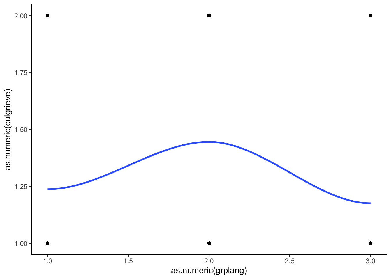
Category 0 compared to Category 2
ggplot(df_MAR %>% filter(culgrieve == "No Grievances Expressed" |
                        culgrieve == "Creating/Strengthening Remedial Policies"),
       aes(x = as.numeric(grplang), y = as.numeric(culgrieve))) +
  geom_point() +
  geom_smooth(method = "loess", se = FALSE) +
  theme_classic()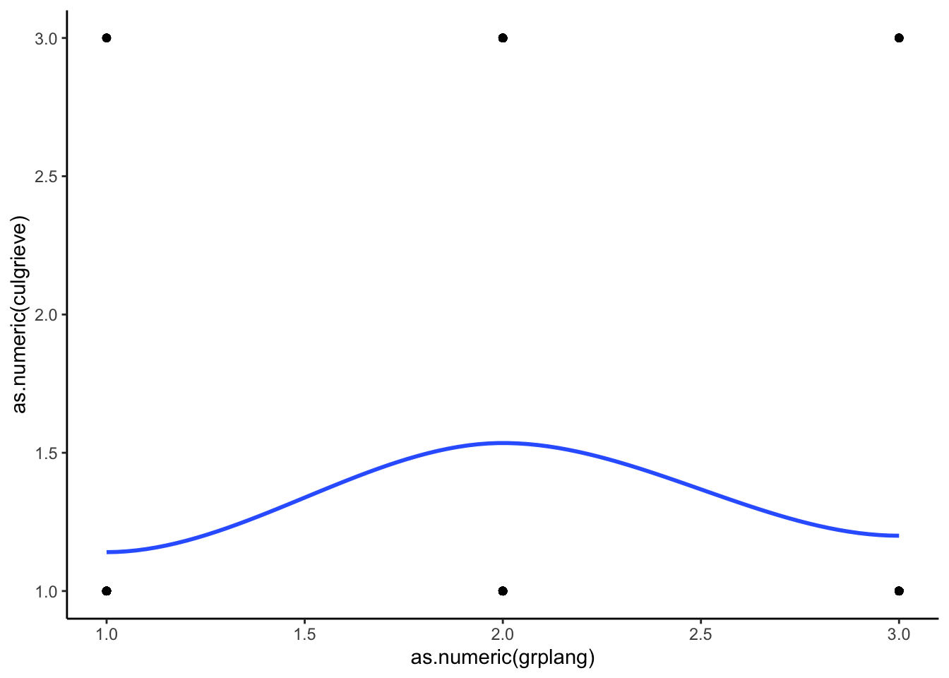
STEP 2: Run your models
Running a multinomial logit command in R is not too difficult. The syntax of the command is the same as other regressions, but instead of using the glm() call,
we’ll use the multinom() function from the nnet package.
First run a basic model with your outcome and key independent variable.
fit_basic <- multinom(culgrieve ~ grplang, data = df_MAR)We have two options for displaying the results of an MLR in R. Our classic summary() function, or a function from the broom package – tidy().
Looking at option 1 below, the results display are flipped from what we are used to. The outcome categories of our dependent variable are the rows and the variable coefficients are the columns. The coefficients and standard errors are stacked on top of each other. It’s a little weird, and it often is difficult to read if the category names are long.
# Option 1 for display
summary(fit_basic)
Call:
multinom(formula = culgrieve ~ grplang, data = df_MAR)
Coefficients:
(Intercept)
Ending Discrimination -1.168166
Creating/Strengthening Remedial Policies -2.581645
grplangSome Speak Native Lang
Ending Discrimination 0.9489541
Creating/Strengthening Remedial Policies 1.5751415
grplangMost Speak Native Lang
Ending Discrimination -0.3786253
Creating/Strengthening Remedial Policies 0.3837751
Std. Errors:
(Intercept)
Ending Discrimination 0.1882289
Creating/Strengthening Remedial Policies 0.3456718
grplangSome Speak Native Lang
Ending Discrimination 0.2108233
Creating/Strengthening Remedial Policies 0.3667327
grplangMost Speak Native Lang
Ending Discrimination 0.2969347
Creating/Strengthening Remedial Policies 0.4605736
Residual Deviance: 1551.835
AIC: 1563.835 If we want our classic display with every X variable as a row in the results table, we can pass the results through the tidy() function with the option to include confidence intervals. The first column is the dependent variable outcome and the second column is the X variable that refer to the coefficient in the estimate column.
# Option 2 for display
tidy(fit_basic, conf.int = TRUE)| y.level | term | estimate | std.error | statistic | p.value | conf.low | conf.high |
|---|---|---|---|---|---|---|---|
| Ending Discrimination | (Intercept) | -1.17 | 0.188 | -6.21 | 5.43e-10 | -1.54 | -0.799 |
| Ending Discrimination | grplangSome Speak Native Lang | 0.949 | 0.211 | 4.5 | 6.76e-06 | 0.536 | 1.36 |
| Ending Discrimination | grplangMost Speak Native Lang | -0.379 | 0.297 | -1.28 | 0.202 | -0.961 | 0.203 |
| Creating/Strengthening Remedial Policies | (Intercept) | -2.58 | 0.346 | -7.47 | 8.11e-14 | -3.26 | -1.9 |
| Creating/Strengthening Remedial Policies | grplangSome Speak Native Lang | 1.58 | 0.367 | 4.3 | 1.75e-05 | 0.856 | 2.29 |
| Creating/Strengthening Remedial Policies | grplangMost Speak Native Lang | 0.384 | 0.461 | 0.833 | 0.405 | -0.519 | 1.29 |
And if you don’t like that you can’t see the full “term” column, you
can use kable() and kable_styling() to display this as an html table.
tidy(fit_basic, conf.int = TRUE) %>%
  kable() %>%
kable_styling("basic", full_width = FALSE)| y.level | term | estimate | std.error | statistic | p.value | conf.low | conf.high |
|---|---|---|---|---|---|---|---|
| Ending Discrimination | (Intercept) | -1.1681661 | 0.1882289 | -6.2060925 | 0.0000000 | -1.5370880 | -0.7992442 |
| Ending Discrimination | grplangSome Speak Native Lang | 0.9489541 | 0.2108233 | 4.5011826 | 0.0000068 | 0.5357480 | 1.3621601 |
| Ending Discrimination | grplangMost Speak Native Lang | -0.3786253 | 0.2969347 | -1.2751132 | 0.2022692 | -0.9606066 | 0.2033559 |
| Creating/Strengthening Remedial Policies | (Intercept) | -2.5816451 | 0.3456718 | -7.4684865 | 0.0000000 | -3.2591494 | -1.9041409 |
| Creating/Strengthening Remedial Policies | grplangSome Speak Native Lang | 1.5751415 | 0.3667327 | 4.2950667 | 0.0000175 | 0.8563585 | 2.2939244 |
| Creating/Strengthening Remedial Policies | grplangMost Speak Native Lang | 0.3837751 | 0.4605736 | 0.8332545 | 0.4047012 | -0.5189327 | 1.2864828 |
Then add in your other covariates.
fit_full <- multinom(culgrieve ~ grplang + trsntlkin + legisrep + execrep +
                       pct_ctry, data = df_MAR)
# Option 1 for display
summary(fit_full)Call:
multinom(formula = culgrieve ~ grplang + trsntlkin + legisrep +
execrep + pct_ctry, data = df_MAR)
Coefficients:
(Intercept)
Ending Discrimination -2.347042
Creating/Strengthening Remedial Policies -3.824512
grplangSome Speak Native Lang
Ending Discrimination 1.146561
Creating/Strengthening Remedial Policies 2.182542
grplangMost Speak Native Lang
Ending Discrimination -0.5749323
Creating/Strengthening Remedial Policies 0.7051977
trsntlkinClose Kindred/Not Adjoining Base
Ending Discrimination 1.302823
Creating/Strengthening Remedial Policies 1.054295
trsntlkinClose Kindred, Adjoining Base
Ending Discrimination 1.0498235
Creating/Strengthening Remedial Policies 0.7401936
trsntlkinClose Kindred, More than 1 Country
Ending Discrimination 0.8770279
Creating/Strengthening Remedial Policies -0.9954818
legisrepYes execrepYes pct_ctry
Ending Discrimination 0.6178156 -0.8255464 0.0005750173
Creating/Strengthening Remedial Policies 0.3123242 -0.2516610 0.0156195847
Std. Errors:
(Intercept)
Ending Discrimination 0.377527
Creating/Strengthening Remedial Policies 0.565078
grplangSome Speak Native Lang
Ending Discrimination 0.2422761
Creating/Strengthening Remedial Policies 0.4199663
grplangMost Speak Native Lang
Ending Discrimination 0.3292604
Creating/Strengthening Remedial Policies 0.4994863
trsntlkinClose Kindred/Not Adjoining Base
Ending Discrimination 0.3015762
Creating/Strengthening Remedial Policies 0.3538105
trsntlkinClose Kindred, Adjoining Base
Ending Discrimination 0.3204507
Creating/Strengthening Remedial Policies 0.3750092
trsntlkinClose Kindred, More than 1 Country
Ending Discrimination 0.3218313
Creating/Strengthening Remedial Policies 0.5044287
legisrepYes execrepYes pct_ctry
Ending Discrimination 0.2034079 0.2131296 0.007023725
Creating/Strengthening Remedial Policies 0.2715894 0.2711577 0.008826351
Residual Deviance: 1427.923
AIC: 1463.923 Oof. There are too many variables for this output to be readable with the summary() command.
So instead let’s just use option 2.
# Option 2 for display
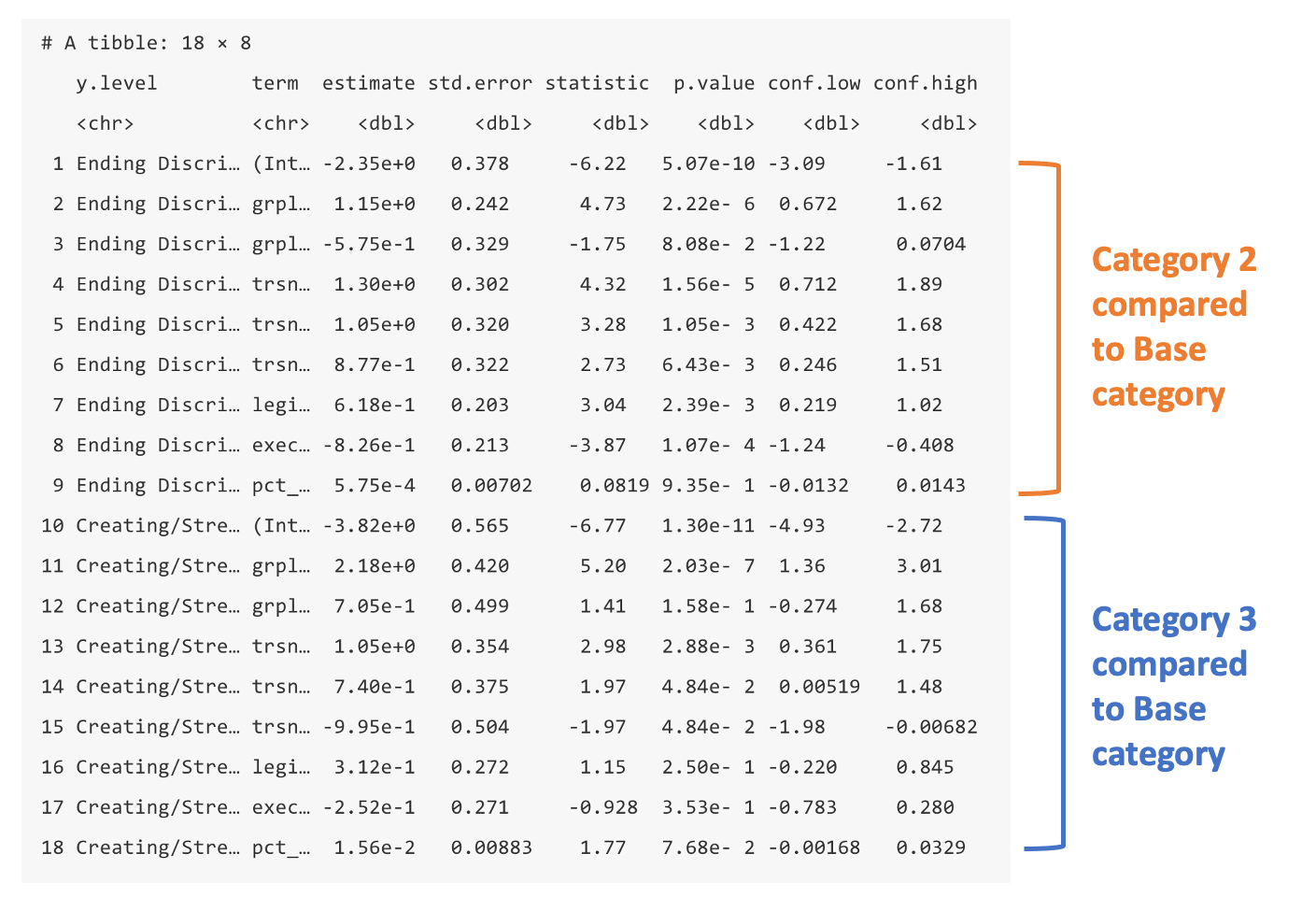
tidy(fit_full, conf.int = TRUE) %>%
kable() %>%
kable_styling("basic", full_width = FALSE)| y.level | term | estimate | std.error | statistic | p.value | conf.low | conf.high |
|---|---|---|---|---|---|---|---|
| Ending Discrimination | (Intercept) | -2.3470420 | 0.3775270 | -6.2168858 | 0.0000000 | -3.0869812 | -1.6071027 |
| Ending Discrimination | grplangSome Speak Native Lang | 1.1465610 | 0.2422761 | 4.7324568 | 0.0000022 | 0.6717087 | 1.6214134 |
| Ending Discrimination | grplangMost Speak Native Lang | -0.5749323 | 0.3292604 | -1.7461322 | 0.0807880 | -1.2202709 | 0.0704064 |
| Ending Discrimination | trsntlkinClose Kindred/Not Adjoining Base | 1.3028231 | 0.3015762 | 4.3200459 | 0.0000156 | 0.7117445 | 1.8939016 |
| Ending Discrimination | trsntlkinClose Kindred, Adjoining Base | 1.0498235 | 0.3204507 | 3.2760842 | 0.0010526 | 0.4217517 | 1.6778954 |
| Ending Discrimination | trsntlkinClose Kindred, More than 1 Country | 0.8770279 | 0.3218313 | 2.7251165 | 0.0064279 | 0.2462501 | 1.5078057 |
| Ending Discrimination | legisrepYes | 0.6178156 | 0.2034079 | 3.0373238 | 0.0023869 | 0.2191435 | 1.0164877 |
| Ending Discrimination | execrepYes | -0.8255464 | 0.2131296 | -3.8734478 | 0.0001073 | -1.2432728 | -0.4078201 |
| Ending Discrimination | pct_ctry | 0.0005750 | 0.0070237 | 0.0818679 | 0.9347518 | -0.0131912 | 0.0143413 |
| Creating/Strengthening Remedial Policies | (Intercept) | -3.8245123 | 0.5650780 | -6.7681142 | 0.0000000 | -4.9320448 | -2.7169798 |
| Creating/Strengthening Remedial Policies | grplangSome Speak Native Lang | 2.1825418 | 0.4199663 | 5.1969450 | 0.0000002 | 1.3594230 | 3.0056607 |
| Creating/Strengthening Remedial Policies | grplangMost Speak Native Lang | 0.7051977 | 0.4994863 | 1.4118459 | 0.1579953 | -0.2737775 | 1.6841729 |
| Creating/Strengthening Remedial Policies | trsntlkinClose Kindred/Not Adjoining Base | 1.0542950 | 0.3538105 | 2.9798299 | 0.0028841 | 0.3608392 | 1.7477507 |
| Creating/Strengthening Remedial Policies | trsntlkinClose Kindred, Adjoining Base | 0.7401936 | 0.3750092 | 1.9738011 | 0.0484044 | 0.0051890 | 1.4751982 |
| Creating/Strengthening Remedial Policies | trsntlkinClose Kindred, More than 1 Country | -0.9954818 | 0.5044287 | -1.9734836 | 0.0484405 | -1.9841440 | -0.0068197 |
| Creating/Strengthening Remedial Policies | legisrepYes | 0.3123242 | 0.2715894 | 1.1499868 | 0.2501493 | -0.2199812 | 0.8446296 |
| Creating/Strengthening Remedial Policies | execrepYes | -0.2516610 | 0.2711577 | -0.9280984 | 0.3533566 | -0.7831203 | 0.2797983 |
| Creating/Strengthening Remedial Policies | pct_ctry | 0.0156196 | 0.0088264 | 1.7696538 | 0.0767848 | -0.0016797 | 0.0329189 |
And finally, look at the full model with relative risk ratios.
Option 1: Use tbl_regression() to exponentiate the coefficients and get a table with relative risk ratios as the coefficients.
tbl_regression(fit_full, exp = TRUE)ℹ Multinomial models have a different underlying structure than the models
gtsummary was designed for. Other gtsummary functions designed to work with
tbl_regression objects may yield unexpected results.| Characteristic | OR1 | 95% CI1 | p-value |
|---|---|---|---|
| Ending Discrimination | |||
| grplang | |||
| <10% Speak Native Lang | — | — | |
| Some Speak Native Lang | 3.15 | 1.96, 5.06 | <0.001 |
| Most Speak Native Lang | 0.56 | 0.30, 1.07 | 0.081 |
| trsntlkin | |||
| No Close Kindred | — | — | |
| Close Kindred/Not Adjoining Base | 3.68 | 2.04, 6.65 | <0.001 |
| Close Kindred, Adjoining Base | 2.86 | 1.52, 5.35 | 0.001 |
| Close Kindred, More than 1 Country | 2.40 | 1.28, 4.52 | 0.006 |
| legisrep | |||
| No | — | — | |
| Yes | 1.85 | 1.25, 2.76 | 0.002 |
| execrep | |||
| No | — | — | |
| Yes | 0.44 | 0.29, 0.67 | <0.001 |
| pct_ctry | 1.00 | 0.99, 1.01 | >0.9 |
| Creating/Strengthening Remedial Policies | |||
| grplang | |||
| <10% Speak Native Lang | — | — | |
| Some Speak Native Lang | 8.87 | 3.89, 20.2 | <0.001 |
| Most Speak Native Lang | 2.02 | 0.76, 5.39 | 0.2 |
| trsntlkin | |||
| No Close Kindred | — | — | |
| Close Kindred/Not Adjoining Base | 2.87 | 1.43, 5.74 | 0.003 |
| Close Kindred, Adjoining Base | 2.10 | 1.01, 4.37 | 0.048 |
| Close Kindred, More than 1 Country | 0.37 | 0.14, 0.99 | 0.048 |
| legisrep | |||
| No | — | — | |
| Yes | 1.37 | 0.80, 2.33 | 0.3 |
| execrep | |||
| No | — | — | |
| Yes | 0.78 | 0.46, 1.32 | 0.4 |
| pct_ctry | 1.02 | 1.00, 1.03 | 0.077 |
|
1
OR = Odds Ratio, CI = Confidence Interval
|
|||
Option 2: Exponentiate within the tidy function
tidy(fit_full, conf.int = TRUE, exponentiate = TRUE) %>%
  kable() %>%
kable_styling("basic", full_width = FALSE)| y.level | term | estimate | std.error | statistic | p.value | conf.low | conf.high |
|---|---|---|---|---|---|---|---|
| Ending Discrimination | (Intercept) | 0.0956517 | 0.3775270 | -6.2168858 | 0.0000000 | 0.0456395 | 0.2004676 |
| Ending Discrimination | grplangSome Speak Native Lang | 3.1473507 | 0.2422761 | 4.7324568 | 0.0000022 | 1.9575793 | 5.0602375 |
| Ending Discrimination | grplangMost Speak Native Lang | 0.5627430 | 0.3292604 | -1.7461322 | 0.0807880 | 0.2951502 | 1.0729441 |
| Ending Discrimination | trsntlkinClose Kindred/Not Adjoining Base | 3.6796699 | 0.3015762 | 4.3200459 | 0.0000156 | 2.0375428 | 6.6452450 |
| Ending Discrimination | trsntlkinClose Kindred, Adjoining Base | 2.8571468 | 0.3204507 | 3.2760842 | 0.0010526 | 1.5246298 | 5.3542754 |
| Ending Discrimination | trsntlkinClose Kindred, More than 1 Country | 2.4037448 | 0.3218313 | 2.7251165 | 0.0064279 | 1.2792194 | 4.5168085 |
| Ending Discrimination | legisrepYes | 1.8548718 | 0.2034079 | 3.0373238 | 0.0023869 | 1.2450099 | 2.7634716 |
| Ending Discrimination | execrepYes | 0.4379956 | 0.2131296 | -3.8734478 | 0.0001073 | 0.2884387 | 0.6650985 |
| Ending Discrimination | pct_ctry | 1.0005752 | 0.0070237 | 0.0818679 | 0.9347518 | 0.9868954 | 1.0144446 |
| Creating/Strengthening Remedial Policies | (Intercept) | 0.0218291 | 0.5650780 | -6.7681142 | 0.0000000 | 0.0072117 | 0.0660740 |
| Creating/Strengthening Remedial Policies | grplangSome Speak Native Lang | 8.8688208 | 0.4199663 | 5.1969450 | 0.0000002 | 3.8939458 | 20.1995576 |
| Creating/Strengthening Remedial Policies | grplangMost Speak Native Lang | 2.0242469 | 0.4994863 | 1.4118459 | 0.1579953 | 0.7605013 | 5.3879926 |
| Creating/Strengthening Remedial Policies | trsntlkinClose Kindred/Not Adjoining Base | 2.8699511 | 0.3538105 | 2.9798299 | 0.0028841 | 1.4345328 | 5.7416735 |
| Creating/Strengthening Remedial Policies | trsntlkinClose Kindred, Adjoining Base | 2.0963414 | 0.3750092 | 1.9738011 | 0.0484044 | 1.0052025 | 4.3719022 |
| Creating/Strengthening Remedial Policies | trsntlkinClose Kindred, More than 1 Country | 0.3695453 | 0.5044287 | -1.9734836 | 0.0484405 | 0.1374983 | 0.9932035 |
| Creating/Strengthening Remedial Policies | legisrepYes | 1.3665977 | 0.2715894 | 1.1499868 | 0.2501493 | 0.8025339 | 2.3271158 |
| Creating/Strengthening Remedial Policies | execrepYes | 0.7775083 | 0.2711577 | -0.9280984 | 0.3533566 | 0.4569779 | 1.3228630 |
| Creating/Strengthening Remedial Policies | pct_ctry | 1.0157422 | 0.0088264 | 1.7696538 | 0.0767848 | 0.9983217 | 1.0334667 |
STEP 3: Interpret your model
Interpretation is the hard part. We’ll practice in the lab together. For each of our four ways to interpret the model, I will interpret the coefficients for one continuous variable (pct_ctry) and one categorical variable (grplang).
Relative Log-Odds
Percent of population:
- Category: Ending Discrimination
- A one unit increase in percent population is associated with a .0006 increase in the log-odds of an ethnocultural group wanting to end discrimination vs having no grievances. It is not statistically significant.
- Category: Creating/Strengthening Remedial Policies
- A one unit increase in percent population is associated with a .0156 increase in the log-odds of an ethnocultural group wanting to create or strengthen remedial policies vs having no cultural grievances. It is not statistically significant.
Language distinctiveness:
- Category: Ending Discrimination
- A group where some medium percentage of members speak the native language (compared to groups where <10% speak the language) is associated with a 1.147 increase in the log-odds of a group wanting to end discrimination compared to having no cultural grievances.
- A group where most members speak the native language (compared to groups where <10% speak the language) is associated with a .575 decrease in the log-odds of a group wanting to end discrimination compared to having no cultural grievances. It is not statistically significant.
- Category: Creating/Strengthening Remedial Policies
- A group where some medium percentage of members speak the native language (compared to groups where <10% speak the language) is associated with a 2.182 increase in the log-odds of a group wanting to create/strengthen remedial policies compared to having no cultural grievances.
- A group where most members speak the native language (compared to groups where <10% speak the language) is associated with a .705 decrease in the log-odds of a group wanting to create/strengthen remedial policies compared to having no cultural grievances. It is not statistically significant.
Relative Risk Ratios
Percent of population:
- Category: Ending Discrimination
- A one unit increase in percent population multiplies the odds of wanting to end discrimination vs having no grievances by 1.0006 (basically 0%). It is not statistically significant.
- Category: Creating/Strengthening Remedial Policies
- A one unit increase in percent population multiplies the odds of wanting to create or strengthen remedial policies vs having no cultural grievances by 1.016 (1.6%). It is not statistically signifcant.
Language distinctiveness:
- Category: Ending Discrimination
- A group where some medium percentage of members speak the native language (compared to groups where <10% speak the language) is multiplies the odds of wanting to end discrimination compared to having no cultural grievances by 3.15 (215%).
- A group where most members speak the native language (compared to groups where <10% speak the language) multiplies the odds of wanting to end discrimination compared to having no cultural grievances by .562 (-43.8%). It is not statistically significant.
- Category: Creating/Strengthening Remedial Policies
- A group where some medium percentage of members speak the native language (compared to groups where <10% speak the language) multiplies the odds of wanting to create/strengthen remedial policies compared to having no cultural grievances by 8.87 (786.8 %).
- A group where most members speak the native language (compared to groups where <10% speak the language) multiplies the odds of wanting to create/strengthen remedial policies compared to having no cultural grievances by 2.02 (102%). It is not statistically significant.
Marginal Effects
The margins() package has difficulty handling multinom results. This is
the closest I can get you to marginal effects for an MLR in R. We are
using the marginaleffects() command from the marginaleffects package.
It does not include marginal effects for the DV reference category for
continuous variables, but I left the results you would get in Stata in
the interpretations below.
NOTE: You must save the results of marginaleffects() as an object and run it
through the summary() command, otherwise the average marginal effects will not
display. You will get a marginal effect for every observation. Heed the warning that the method of producing standard errors are different from Stata.
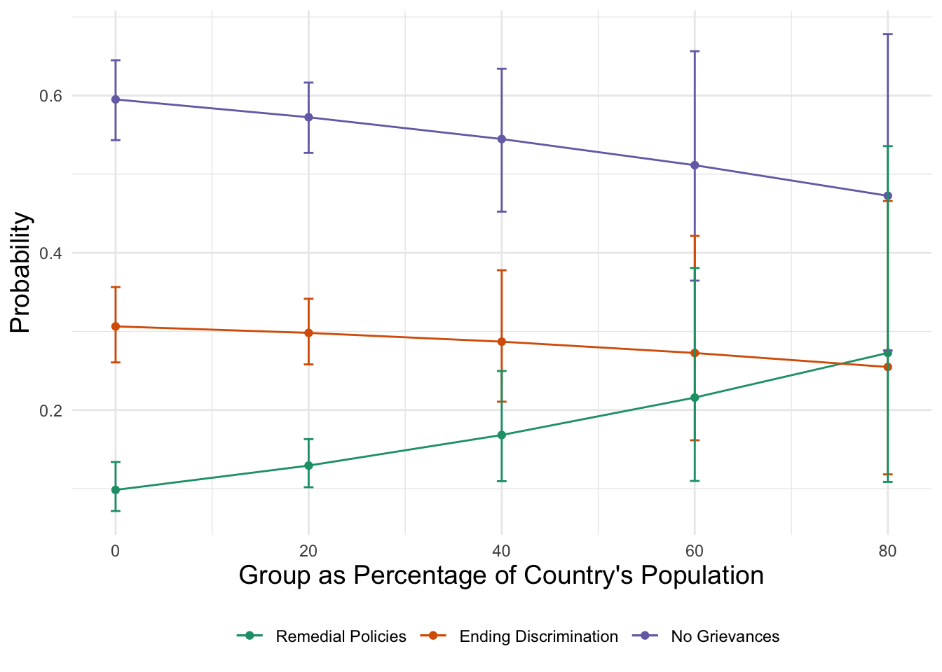
Percent of population:
mfx_pct_ctry <- marginaleffects(fit_full, variables = "pct_ctry", type = "probs")Warning: The standard errors estimated by `marginaleffects` do not match those
produced by Stata for `nnet::multinom` models. Please be very careful when
interpreting the results.summary(mfx_pct_ctry)| type | group | term | estimate | std.error | statistic | p.value | conf.low | conf.high |
|---|---|---|---|---|---|---|---|---|
| probs | Creating/Strengthening Remedial Policies | pct_ctry | 0.00171 | 0.00182 | 0.939 | 0.348 | -0.00186 | 0.00527 |
| probs | Ending Discrimination | pct_ctry | -0.000611 | 0.00223 | -0.274 | 0.784 | -0.00498 | 0.00376 |
Category 1: No Grievances
- A one unit increase in the percent the group represents in the total population is associated with a .001 descrease in the probability that the group has no grievances.
Category 2: Ending Discrimination
- A one unit increase in the percent the group represents in the total population is associated with a .0006 decrease in the probability that the group wants to end discrimination.
Category 3: Creating/Strengthening Remedial Policies
- A one unit increase in the percent the group represents in the total population is associated with a .002 increase in the probability that the group wants to create or strengthen remedial policies.
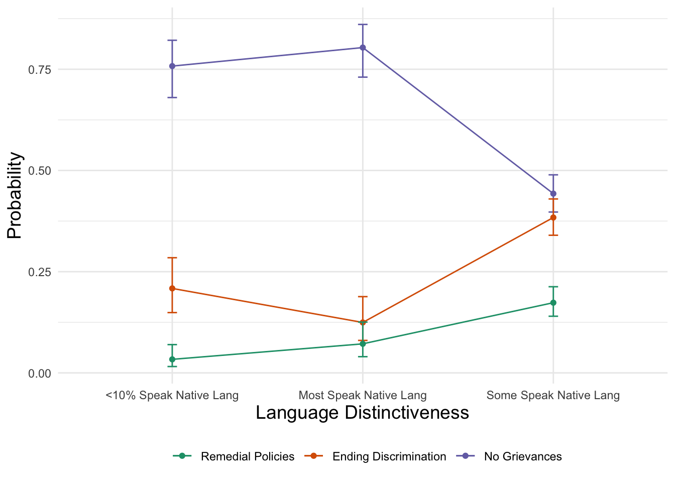
Language Distinctiveness:
mfx_grplang <- marginaleffects(fit_full, variables = "grplang", type = "probs")
summary(mfx_grplang) | type | group | term | contrast | estimate | std.error | statistic | p.value | conf.low | conf.high |
|---|---|---|---|---|---|---|---|---|---|
| probs | Creating/Strengthening Remedial Policies | grplang | Most Speak Native Lang - <10% Speak Native Lang | 0.0458 | 0.0335 | 1.37 | 0.172 | -0.0199 | 0.112 |
| probs | Creating/Strengthening Remedial Policies | grplang | Some Speak Native Lang - <10% Speak Native Lang | 0.15 | 0.0284 | 5.3 | 1.15e-07 | 0.0947 | 0.206 |
| probs | Ending Discrimination | grplang | Most Speak Native Lang - <10% Speak Native Lang | -0.087 | 0.0101 | -8.62 | 0 | -0.107 | -0.0673 |
| probs | Ending Discrimination | grplang | Some Speak Native Lang - <10% Speak Native Lang | 0.157 | 0.011 | 14.3 | 0 | 0.135 | 0.178 |
| probs | No Grievances Expressed | grplang | Most Speak Native Lang - <10% Speak Native Lang | 0.0412 | 0.0327 | 1.26 | 0.207 | -0.0228 | 0.105 |
| probs | No Grievances Expressed | grplang | Some Speak Native Lang - <10% Speak Native Lang | -0.307 | 0.026 | -11.8 | 0 | -0.358 | -0.256 |
Category 1: No Grievances
- A group where some medium percentage of members speak the native language (compared to groups where <10% speak the language) is associated with a .307 decrease in the probability of having no grievances.
- A group where most members speak the native language (compared to groups where <10% speak the language) is associated with a .041 increase in the probability of having no grievances. It is not statistically significant.
Category 2: Ending Discrimination
- A group where some medium percentage of members speak the native language (compared to groups where <10% speak the language) is associated with a .157 increase in the probability of wanting to end discrimination.
- A group where most members speak the native language (compared to groups where <10% speak the language) is associated with a .087 decrease in the probability of wanting to end discrimination. It is not statistically significant.
Category 3: Creating/Strengthening Remedial Policies
- A group where some medium percentage of members speak the native language (compared to groups where <10% speak the language) is associated with a .150 increase in the probability of wanting to create or strengthen remedial policies.
- A group where most members speak the native language (compared to groups where <10% speak the language) is associated with a .045 increase in the probability of wanting to create/strengthen remedial policies. It is not statistically significant.
Predicted Probabilities
Because in class you all pointed out the difficulties of reading these plots because of the formatting, I decided to format these using some of the tips we learned (go to the graph fundamentals lab for code to install).
Percent of Population
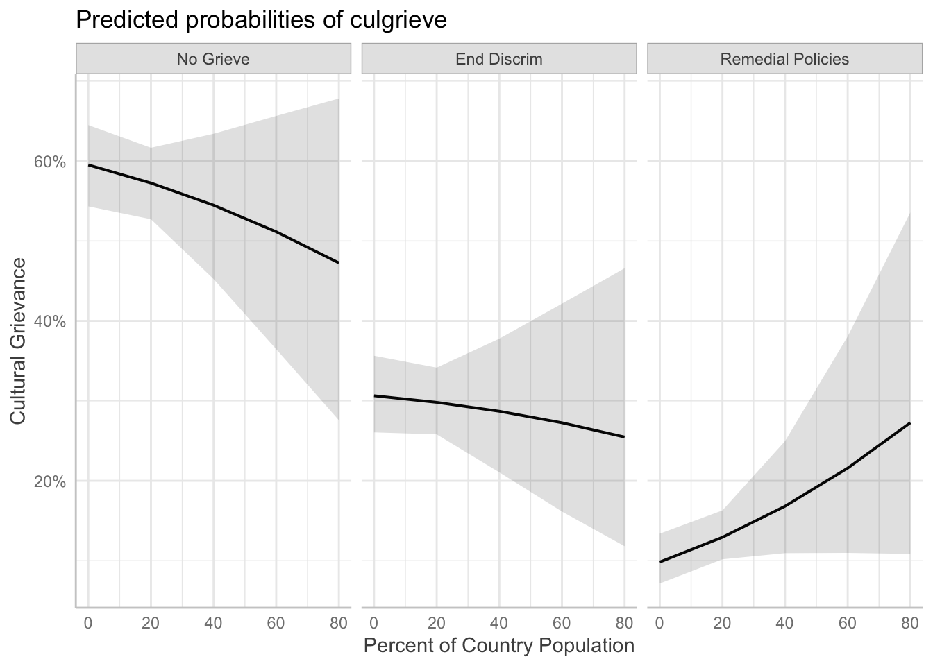
This is the basic plotting with ggeffects. It produces a 3 panel plot by default.
ggeffect(fit_full, terms = "pct_ctry[0:80 by = 20]") %>%
    plot()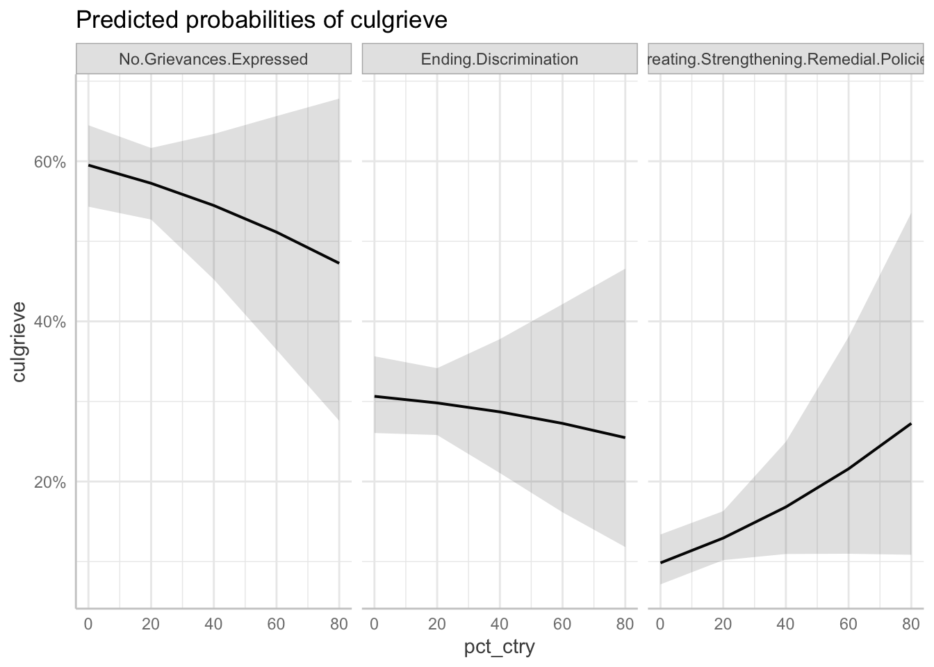
The plot has some less than ideal features, namely that we can’t read the facet plot titles. If you like the three plots next to each other, you can just alter the facet titles:
# Create a basic plot
basic <- ggeffect(fit_full, terms = "pct_ctry[0:80 by = 20]") %>%
  plot()

# Prep facet labels
response.labs <- c("No Grieve", "End Discrim", "Remedial Policies")
names(response.labs) <- c("No.Grievances.Expressed", "Ending.Discrimination",
                          "Creating.Strengthening.Remedial.Policies")

basic +
  # Change the facet labels
  facet_wrap(~ response.level,
             labeller = labeller(response.level = response.labs)) +
  labs(
    y = "Cultural Grievance",
    x = "Percent of Country Population"
  )
Now, you may just want a single plot with all three lines. That’s hard to do with the basic plotting function built into geffects. So we can build it ourselves. ggeffects plotting relies on ggplot(), code, so we can build it manually. This is a relatively complicated bit of code, but I annotated each line for you.
# Save the predicted probabilities
  pprob_pct_ctry <- ggeffect(fit_full, terms = "pct_ctry[0:80 by = 20]")

# Build the plot with ggplot manually
# The aesthetics refer to variable names in the ggeffects saved results
# We are grouping the plot by the "response.level" of our outcome.
  ggplot(data = pprob_pct_ctry, aes(x = x, y = predicted,
               color = response.level, group = response.level)) +
    # Add line layer
    geom_line() +
    # Add point layer
    geom_point() +
    # Add confidence intervals as error bars
    geom_errorbar(aes(ymin = conf.low, ymax = conf.high,
                    color = response.level,
                    group = response.level),
                  width = 1) +
    # Change the color of the lines, remove legend title, change the
    # labels of the lines in the legend.
    scale_color_brewer(palette = "Dark2",
                       name = "",
                       labels = c("Remedial Policies",
                                  "Ending Discrimination",
                                  "No Grievances")) +
    # Add titles to the x and y axis
    labs(
      x = "Group as Percentage of Country's Population",
      y = "Probability"
    ) +
    # Set the theme
    theme_minimal() +
    theme(
      legend.position = "bottom", # move legend to the bottom
      axis.title = element_text(size = 14) # increase axis title size
      )
Language Distinctiveness
Just like above we can produce a basic plot with panels. For categorical variables, ggeffects does not draw a line plot, just points with confidence intervals.
ggeffect(fit_full, terms = "grplang") %>%
  plot()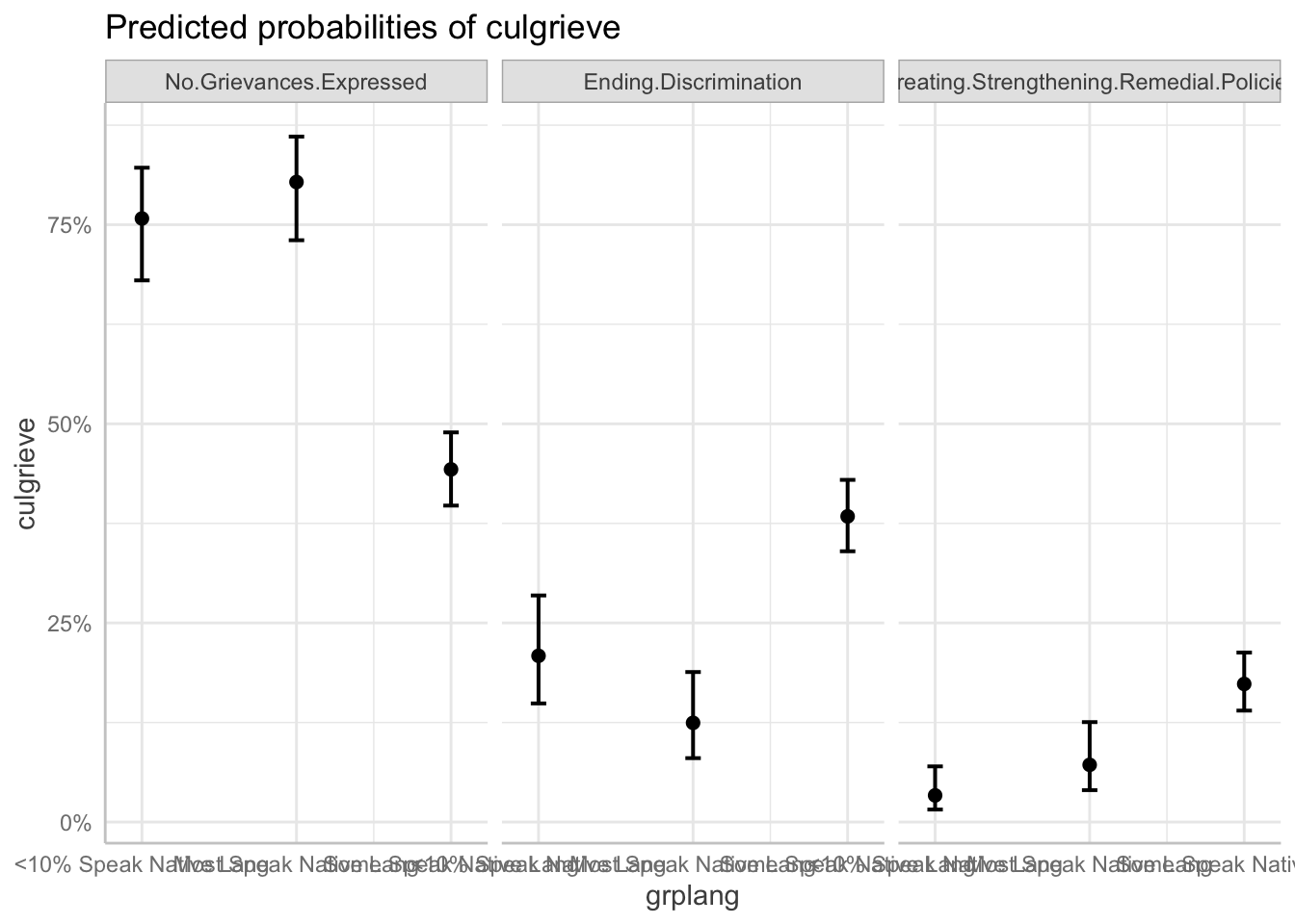
And then we can also build the plot manually.
# Save results
pprob_grplang <- ggeffect(fit_full, terms = "grplang")

# Build plot
ggplot(data = pprob_grplang,
       aes(x = x, y = predicted,
           color = response.level, group = response.level)) +
  geom_line() +
  geom_point() +
  geom_errorbar(aes(ymin = conf.low, ymax = conf.high,
                    color = response.level,
                    group = response.level),
                width = .05) +
  scale_color_brewer(palette = "Dark2",
                     name = "",
                     labels = c("Remedial Policies",
                                "Ending Discrimination",
                                "No Grievances")) +
  labs(
    x = "Language Distinctiveness",
    y = "Probability"
  ) +
  # Set the theme
  theme_minimal() +
  theme(
    legend.position = "bottom", # move legend to the bottom
    axis.title = element_text(size = 14) # increase axis title size
  )
STEP 4: Check your assumptions
To keep this lab from being too long and because the way you check assumptions carries over from logistic regression, I am not going to include them in this lab.
But if we were checking for the independence of irrelevant alternatives (IIA) assumption, we would want to make sure that we were sure ending discrimination and remedial policies are truly distinct categories.
15.4 Wald Test for MLR
Overall, the Wald test is identical to what you would do for all the other models. The one thing that is different, however, is that the name of coefficients are a little different given multiple outcome categories. We have to reference the outcome category label followed by the coefficient variable name. Beyond this, we interpret the Wald test the same way we do in previous contexts.
Test if adding pct_ctry has an effect for both outcomes
linearHypothesis(fit_full,
                 c("Ending Discrimination:pct_ctry = 0",
"Creating/Strengthening Remedial Policies:pct_ctry = 0"))| Df | Chisq | Pr(>Chisq) |
|---|---|---|
| 2 | 3.29 | 0.193 |
Test whether the coefficients for pct_ctry for each outcome are statistically different
linearHypothesis(fit_full,
                   c("Ending Discrimination:pct_ctry =
Creating/Strengthening Remedial Policies:pct_ctry"))| Df | Chisq | Pr(>Chisq) |
|---|---|---|
| 1 | 2.4 | 0.121 |
Test if adding legisrep has an effect
linearHypothesis(fit_full,
                   c("Ending Discrimination:legisrepYes = 0",
"Creating/Strengthening Remedial Policies:legisrepYes = 0"))| Df | Chisq | Pr(>Chisq) |
|---|---|---|
| 2 | 9.24 | 0.00984 |
Test whether the coefficients for legisrep for each outcome are statistically different
linearHypothesis(fit_full,
                   c("Ending Discrimination:legisrepYes =
Creating/Strengthening Remedial Policies:legisrepYes"))| Df | Chisq | Pr(>Chisq) |
|---|---|---|
| 1 | 1.2 | 0.273 |