Chapter 5 Histogram
Quantitative variables often take so many values that a graph of the distribution is clearer if nearby values are group together. The most common graph of the distribution of one quantitative variable is a histogram. (Used for continious type of data)
Histogram can be used for continious type of random variables
to find out the shape of the distribution of the variable of interest.
to detect the outlier.
5.1 How to draw a histogram in base R?
Let’s consider mtcars data set being available in R.
hist(mtcars$mpg)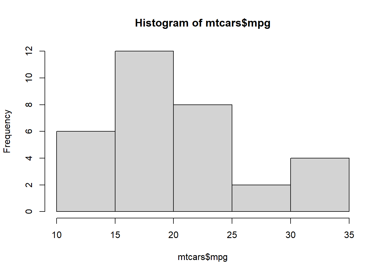
hist(mtcars$mpg, breaks=10)#Specify approximate number of bins with breaks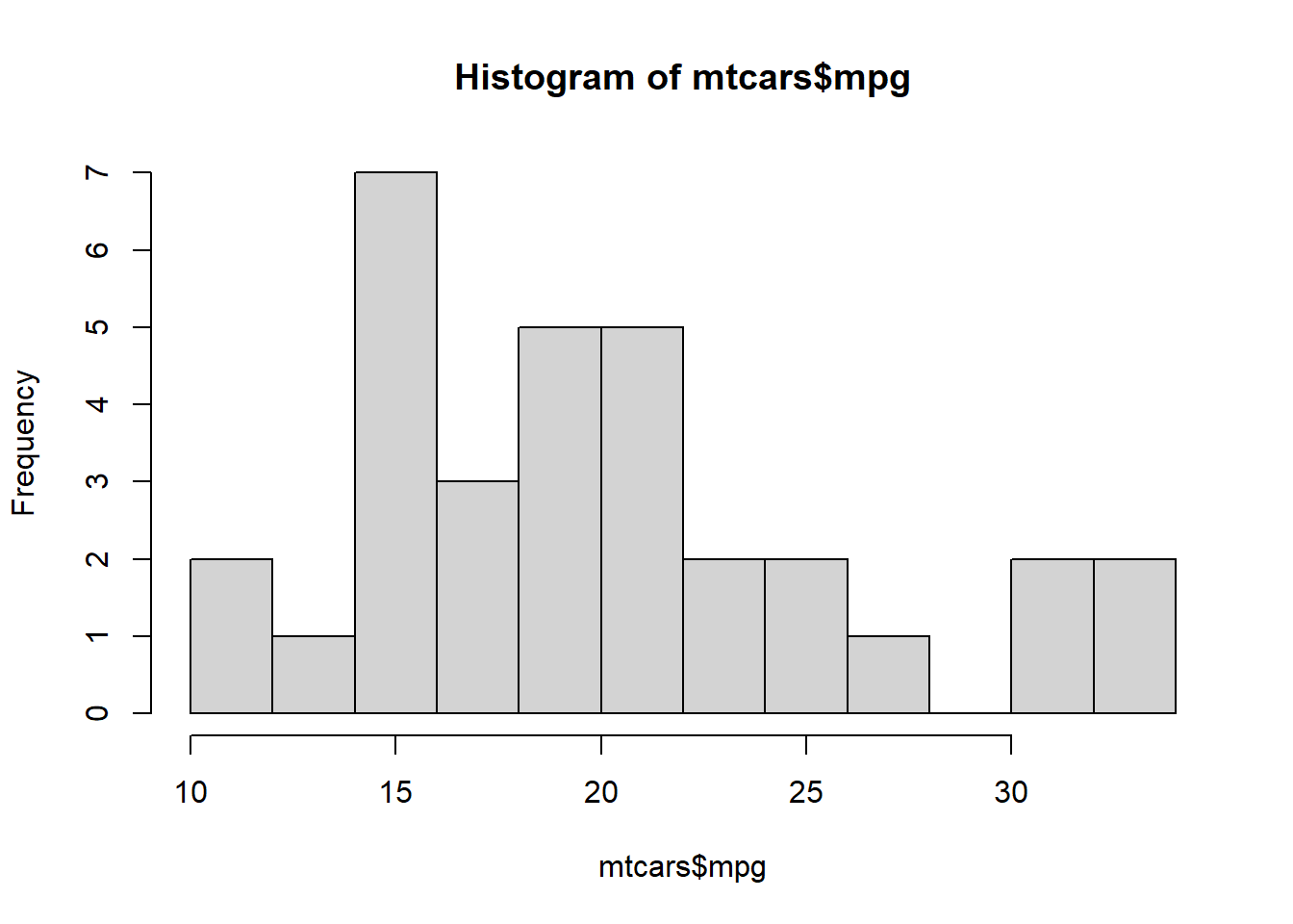
5.2 How can we draw histogram in ggplot2?
qplot(mtcars$mpg)## `stat_bin()` using `bins = 30`. Pick better value with `binwidth`.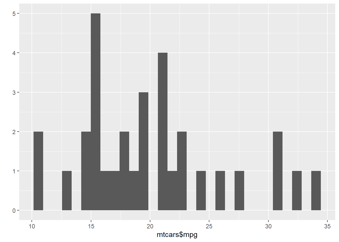
If the vector is in a data frame, you can use the following syntax:
qplot(mpg, data=mtcars, binwidth=4)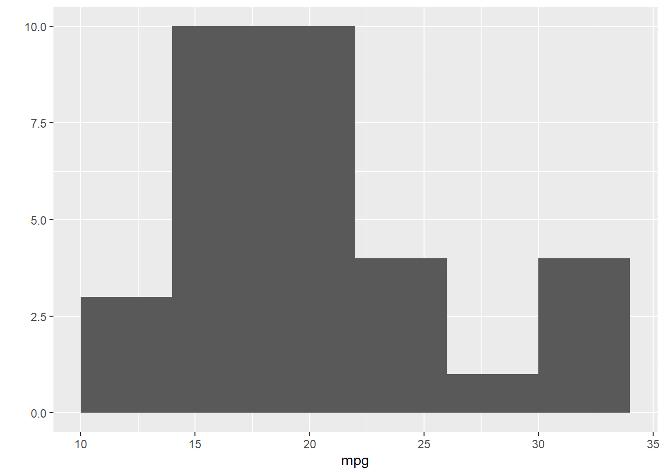
This is equivalent to:
ggplot(mtcars, aes(x=mpg)) + geom_histogram(binwidth=4)#geom_histogram converts your plot into histogram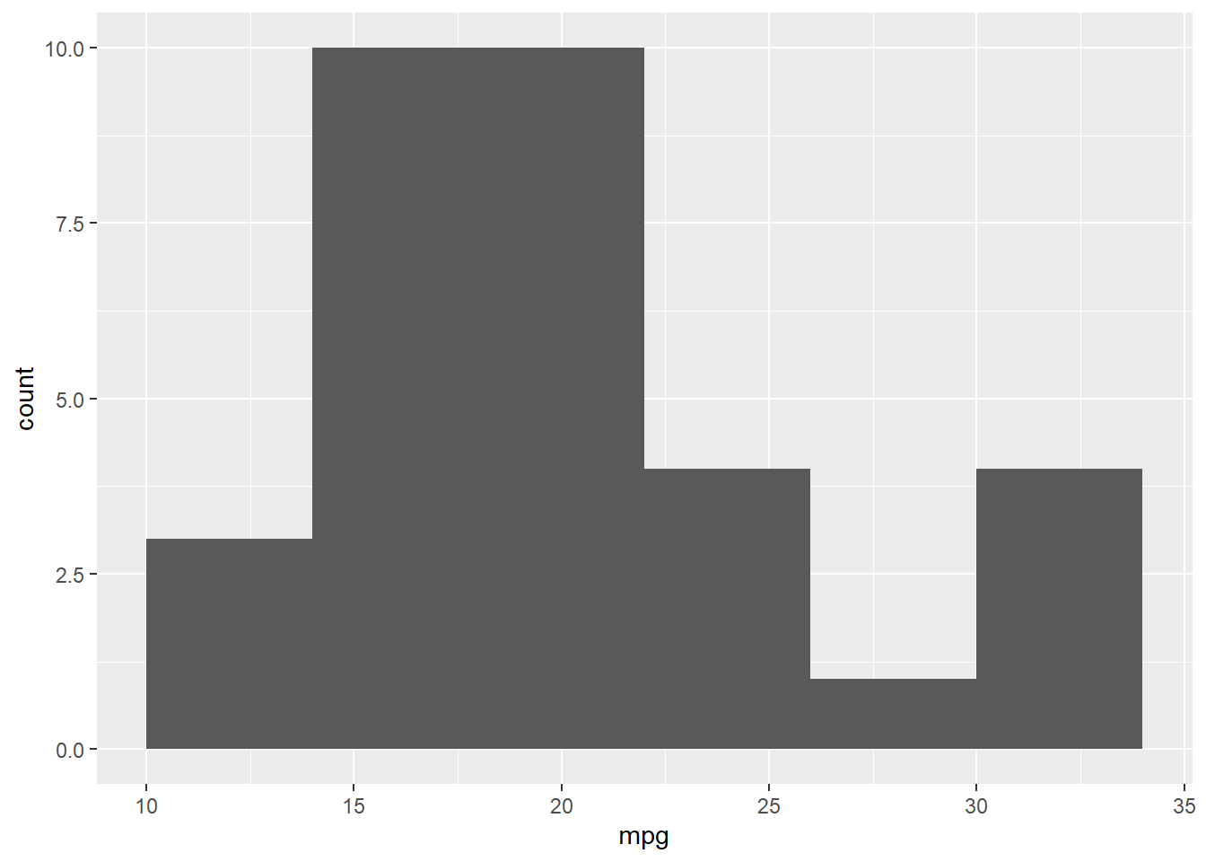
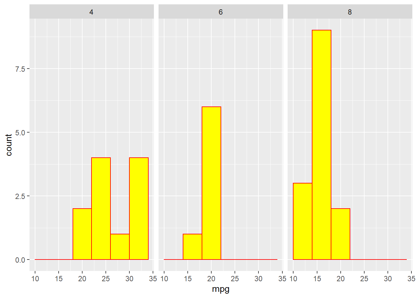
ggplot(mtcars,aes(x=mpg))+geom_histogram(binwidth = 4,colour="red",fill="yellow")#with color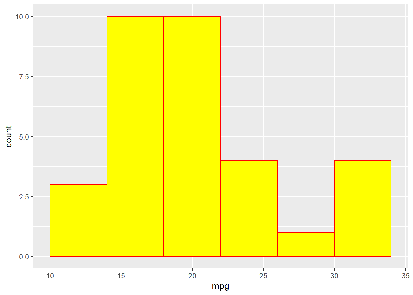
#fill fills inside of histogram
#colour defines the color of frame
This way is the better one.