Chapter 10 Special topic: Clinical Trial Data Analysis with R

Nhan Thi Ho, MD, PhD

10.1 Clinical trial design

10.1.1 Fundamentals of major randomized controlled trial design

Choice of patients, centers	Choice of treatments	Choice of outcomes	Randomization	Blinding	Trial sample size
- Precise eligibility criteria - Multi-center trial is preferable - Appropriate geographic representation	- Precise treatment regimens - Placebo control or active comparator - 3-arm-trial may sometimes be appropriate	- Define the primary efficacy endpoint - Select components of composite primary endpoint - List secondary endpoints - Define safety endpoints	- Allocation concealment - Proper statistical method for randomization - Ensure between group balance by stratification - Unequal randomization may be useful for new treatment	- Double blind if practical - If not practical, blinded evaluation is essential - Blinding is important for soft endpoints	- Sample size calculation using appropriate method - Anticipate realistic effect size - Compromise may be needed for a real world study - Determining needed number of events may be useful

(Source: adapted from Pocock S.J et al. J Am Coll Cardiol. 2015;66(24):2757-66. (Pocock, McMurray, and Collier 2015))

10.1.2 Requirements

Clinical trial design should accomplish the following (Piantadosi 2005):

Quantify and reduce errors due to chance
Reduce or eliminate bias
Yield clinically relevant estimates of effects and precision
Be simple in design and analysis
Provide a high degree of credibility, reproducibility, and external validity
Influence future clinical practice

10.1.3 Common concepts

One-way designs: Only one factor= treatment
Two-way factorial design: various combinations of interventions
Parallel design =typical design: patients are randomized to a treatment and remain on that treatment throughout the course of the trial.
Randomization: is used to remove systematic error (bias) and to justify Type I error probabilities in experiments; an essential feature of clinical trials for removing selection bias.
Selection bias: occurs when a physician decides treatment assignment and systematically selects a certain type of patient for a particular treatment.
Blocking and stratification are used to control unwanted variation.
Placebos or relevant controls.
Treatment masking or blinding is an effective way to ensure objectivity of the person measuring the outcome variables. Double-masked: both investigators and patients are masked to the treatment. Single-masked: only patients or evaluators are masked (Friedman et al. 2015).

10.1.4 Nonrandomized Studies

10.1.4.1 Nonrandomized Concurrent Control Studies

No randomization
May match by some characteristics
Bias in the allocation of participants to either the intervention or control group
Possible: one center= one group

$\rightarrow$ Analysis:

Baseline comparison + testing
Adjusting for covariates

10.1.4.2 Historical Controls and Databases

Nonrandomized and nonconcurrent.

All new participants can receive the new intervention
Historical control data can be obtained from two sources: literature, unpublished $\rightarrow$ low quality, uncomparable
Prone to bias

$\rightarrow$ Analysis:

Two sample comparison/ one sample comparing to constant
Baseline comparison + testing
Adjusting for covariates

10.1.5 Cross-Over Designs

Special case of a randomized control trial.

Each participant to serve as his own control.
In the simplest case (two period cross-over design): each participant will receive either intervention or control (A or B) in the first period and the alternative in the succeeding period. The order in which A and B are given to each participant is randomized $\rightarrow$ approximately half of the participants receive the intervention in the sequence AB and the other half in the sequence BA. This is so that any trend from first period to second period can be eliminated in the estimate of group differences in response.
There may be more than two periods, a wash-out period may be used between the periods.

10.1.5.1 Advantages

Allows assessment of how each participant does on both A and B.
Reduction in variability because the measured effect of the intervention is the difference in an individual participant’s response to intervention and control $\rightarrow$ need smaller sample sizes to detect a specific difference in response (parallel or noncross-over designs need 2.4 times bigger in sample size)

10.1.5.2 Strict assumption

The effects of the intervention during the first period must not carry over into the second period

10.1.5.3 Analysis: Significance tests

Carry-over: Is the carry-over from A to B (group 1 2nd period) the same as from B to A (group 2 2nd period)? The null hypothesis being tested is that the carry-over effects are equal between groups 1 (A first) and group 2 (B first).
Treatment: Note: We can only test the treatment effect if it can be assumed that the carryover effects are equal. Hence it is necessary to perform the test above first. If a significant difference is found in carry-over, then this subsequent test will be invalid. The null hypothesis being tested is that the treatment effects are equal.
Period: test the period effect (i.e., is there a change over time irrespective of treatment) $\rightarrow$ need to assume that there is no significant treatment effect. The null hypothesis being tested is that changes between treatments are equal irrespective of time.

10.1.6 Factorial Design

Test the effect of more than one treatment, permits an assessment of potential interactions among the treatments.
Analysis: multiple comparison.

10.1.7 Group Allocation Designs

A group of individuals, a clinic or a community are randomized to a particular intervention or control.

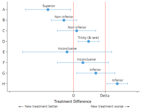
10.1.8 Studies of Equivalency and Noninferiority

Demonstrate that the new intervention is not worse, in terms of the primary response variable, than or at least as good as the standard by some predefined margin. (Usually, many clinical trials are designed to demonstrate that a new intervention is better than or superior to the control).

The control or standard treatment must have been shown conclusively to be effective.

Possible results of noninferiority trials:

10.2 Sample size- power

The underlying theme of sample size calculation in all clinical trials is precision. Two circumstances:

Precision for an estimator (e.g. 95% confidence interval).
Statistical power for hypothesis testing, e.g., requiring 0.80 or 0.90 statistical power (1- $\beta$ ) for a hypothesis test when the significance level ( $\alpha$ ) is 0.05 to detect the desired effect size (the clinically meaningful effect) (Chow et al. 2017).

10.2.1 Some R packages

Package “SampleSize4ClinicalTrials” (Qi and Zhu 2021)

Examples:

#install.packages("SampleSize4ClinicalTrials")
library("SampleSize4ClinicalTrials")
#Comparing blood glucose (mmol/l) in treatment vs. placebo, superior design 
ssc_meancomp(design=2L, ratio=1, alpha=0.05, power=0.8, sd=2, theta=1, delta=0.5)

##   Treatment Control
## 1       198     198

10.3 Randomization

Randomization tends to produce study groups comparable with respect to known as well as unknown risk factors, removes investigator bias in the allocation of participants, and guarantees that statistical tests will have valid false positive error rates.

Simple: a patient is assigned a treatment without any regard for previous assignments (~fliping coin)
Randomization in permuted blocks
Stratified Randomization
Adaptive randomization refers to any scheme in which the probability of treatment assignment changes according to assigned treatments of patients already in the trial.

10.3.1 R package

randomizeR An R Package for the Assessment and Implementation of Randomization in Clinical Trials.

Examples:

#install.packages("randomizeR")
library(randomizeR)
# generate randomization sequences using the Random Allocation Rule for N = 50
myPar <- rarPar(50)
genSeq(myPar)

## 
## Object of class "rRarSeq"
## 
## design = RAR 
## seed = 99276 
## N = 50 
## groups = A B 
## 
## The sequence M: 
## 
## 1 A   A   B   A   B   B   A   B   B   B   ...

10.4 Interim Analysis

10.4.1 Overview

“Interim analysis” or “early stopping” procedures are used to interpret the accumulating information during a clinical trial to monitor treatment effects as well as tracking safety issues. Reasons stopping a trial can be:

Treatments are found to be convincingly different,
Treatments are found to be convincingly not different,
Side effects or toxicity are too severe to continue treatment, relative to the potential benefits,
The data are of poor quality,
Accrual is too slow to complete the study in a timely fashion,
Definitive information is available from outside the study, making the trial unnecessary or unethical, this is also related to the next item…
The scientific questions are no longer important because of other developments,
Adherence to the treatment is unacceptably poor, preventing an answer to the basic question,
Resources to perform the study are lost or no longer available, and/or
The study integrity has been undermined by fraud or misconduct.

“The review, interpretation, and decision-making aspects of clinical trials based on interim data are necessary but prone to error. If the investigators learn of interim results, then it could affect objectivity during the remainder of the trial, or if statistical tests are performed repeatedly on the accumulating data, then the Type I error rate is increased”.

10.4.2 Methods used in interim analysis

“Although many statistical techniques are available to assist in monitoring, none of them should be used as the sole basis in the decision to stop or continue the trial”.

Likelihood Methods
Bayesian Methods
Frequentist Methods: O’Brien-Fleming, Pocock, Haybittle-Peto
Alpha Spending Function approach
Futility Assessment with Conditional Power; Adaptive Designs

For details, please see Courses: Design and Analysis of Clinical Trials

10.4.3 Monitoring and Interim Reporting for Trials

10.4.3.1 Single-Center Trials

The report should include:

Compliance with governmental and institutional oversight,
Review of eligibility (low frequency of ineligible patients entering the trial),
Treatment review (most patients are adhering to the treatment regimen),
Summary of response,
Summary of survival,
Adverse events,
Safety monitoring rules (possibly statistical criteria for evaluating safety endpoints), and
Audit and other quality assurance reviews.

10.4.3.2 Multi-Center Trials

A DSMB typically examines the following issues:

Are the treatment groups comparable at baseline?
Are the accrual rates meeting initial projections and is the trial on its scheduled timeline?
Are the data of sufficient quality?
Are the treatment groups different with respect to safety and toxicity data?
Are the treatment groups different with respect to efficacy data?
Should the trial continue?
Should the protocol be modified?
Are other descriptive statistics, graphs, or analyses needed for the DSMB to make its decisions?

10.5 Estimating Clinical Effects

10.5.1 Dose-Finding (Phase I) Studies

What level of the drug is appropriate? $\rightarrow$ Assess the distribution and elimination of drug in the human system.

Pharmacokinetic (PK) models (compartmental models): to account for the absorption, distribution, metabolism, and excretion of a drug in the human system.

10.5.2 Safety and Efficacy (Phase II) Studies

The main objectives is to estimate the frequency of adverse reactions and estimate the probability of treatment success: often are expressed in binary form, presence/absence of adverse reaction, success/failure of treatment, etc.,. Three common parameters of risk:

Risk difference
Relative risk
Odds ratio

Statistical test of the null hypothesis H0: RR = 1 (or H0: RD = 0).
If safety and efficacy study is stratified according to some factor, such as clinical center, disease severity, gender, etc $\rightarrow$ estimate the odds ratio while accounting for strata effects. Mantel-Haenszel Test for the Odds Ratio: assumes that the odds ratio is equal across all strata, although the rates, p1 and p2, may differ across strata $\rightarrow$ calculates the odds ratio within each stratum and then combines the strata estimates into one estimate of the common odds ratio.
In some safety and efficacy studies, it is of interest to determine if an increase in the dose yields an increase (or decrease) in the response $\rightarrow$ dose-response or trend analysis.

Continuous response: Jonckheere-Terptsra (JT) trend test which is based on a sum of Mann-Whitney-Wilcoxon tests.
Binary response: Cochran-Armitage (CA) trend test

Survival Analysis For time-to-event outcomes: Kaplan-Meier survival curve (log rank test) (Pocock, McMurray, and Collier 2015).

10.5.3 Comparative Treatment Efficacy (Phase III) Trials

Statistical methods used are based on types of outcomes

Contiunous
Categorical
Time-to-event
…

It’s time to review what you have learn throughout this book !

10.6 Clinical Trial Analysis and reporting

10.6.1 Baseline Assessment

10.6.1.1 Description of Trial Participants

The typical Table 1 of the results publication. It provides documentation that can guide cautious extrapolation of trial findings to other populations with the same medical condition

10.6.1.2 Controlling for Imbalances in the Analysis

Imbalanced groups at baseline may be addressed by covariate-adjustment during analysis.

10.6.1.3 Subgrouping

Stratified analysis: help to identify the speciﬁc population most likely to beneﬁt from, or be harmed by, the intervention; elucidate the mechanism of action of the intervention. Deﬁnition of such subgroups should rely only on baseline data, not data measured after initiation of intervention (except for factors such as age or gender which cannot be altered by the intervention).

10.6.2 Trial profile

Figure shows the ﬂow of patients through the trial from the pre-randomization build-up to the post-randomization follow-up.

10.6.3 Tables/ plots of main outcomes

The key table for any clinical trial displays the main outcomes by treatment group.
The most common type of figure in trial is Kaplan-Meier plot of time-to-event outcomes, repeated measures over time (longitudinal data)

10.6.4 Estimates of treatment effects and their CIs

Effect size (point estimate)
Uncertainty (CIs)

10.6.4.1 p values and interpretation

Should provide actual p value (not <)
Useful to recognize the link between the p value and the 95% CI for the treatment difference
Use 2-sided p values
A small p value clariﬁes that an observed treatment difference appears greater than what could be attributed to chance, but this does not automatically mean that a real treatment effect is occurring (There may be biases in the study design and conduct).
There is an important distinction between statistical signiﬁcance and clinical relevance of a treatment effect $\rightarrow$ The magnitude of treatment difference and its CI are a guide for clinical usefulness of treatment difference.
For a small trial the magnitude of treatment needs to be very large to reach a statistically signiﬁcant treatment effect.

10.6.5 Summary

The main steps in data analysis and reporting for clinical trials:

What to include in result section

Trial profile
Baseline characteristics
Main outcomes tables +/- figures

Quantify association, uncertainty and evidence: estimate treatment effect (e.g. relative risk, odds ratio, absolute difference, number needed to treat, hazard ration for time to event outcomes, …), confidence interval and p-values.

10.6.6 Statisticial Controversy in Reporting of Clinical Trials

Problems and solutions:

Problems	Solution
Multiplicity of data: how to make sense of all the options?	- Predefined Statistical Analysis Plan (SAP) - Prioritized primary endpoint - Balanced account of safety and efficacy - Careful interpretation of composite endpoints
Covariate adjustment: should key results be adjusted for baseline covariates?	- Adjust variables affecting prognosis - Predefined chosen variables and models - Consider covariate adjustment as primary analysis
Subgroup analysis: which subgroups should be explored?	- Predefined subgroups - Analyse using interaction tests not subgroup p-values - Interprete all subgroup findings cautiously
Individual benefits and risks: how to link trial findings to individualized patient care?	- Balance absolute benefits against absolute harms - Consider individual risk profile in determine their treatment benefit - Consider multivariable model instead of univariable subgroups
Intention to treat (ITT) analysis: how to deal with non-adherence during follow-up	- Prioritize ITT analysis - Continue follow up for patients withdrawing from treatment if possible - Minimize poor compliance and loss of follow-up - For non-inferiority trial, present both ITT and per protocol analyses
Interpreting surprising results: what to do with unexpected findings?	- Seek evidence to confirm (or not) as soon as possible - Be skeptical of large effects - Anticipate regression to the truth - Avoid alarmist reactions to unexpected safety signals

10.6.7 Examples of real clinical trial data analysis and reporting using R

Below are some journal articles for clinical trials analyzed by the author Nhan Thi Ho et al. using R.

10.7 Case study

The data for the examples below are from a multi-centered phase 1/2/3 COVID-19 vaccine trial in which the author Nhan Thi Ho participated as a core researcher/ data scientist (N. T. Ho et al. 2024). The actual interim and final analyses for this trial for publication and authority approval were done in SAS. A sample of trial data (with some modification for de-identification) are used in the following examples to demonstrate the use of R for clinical trial data analysis and report. The example data contain the following datasets:

ran.ex: randomization list and analysis sets
base.ex: baseline data
ve.ex: time to event outcome (COVID-19) data
sae.ex: serious adverse event data
ae.ex: adverse event data

10.7.1 Load required packages and example data

#load multiple packages
Packages <- c("knitr","rmarkdown","kableExtra","tidyverse","r2rtf","rio","arsenal",
              "sas7bdat","foreign","stringr","lubridate","survival",
              "survminer","gridExtra","Hmisc")
lapply(Packages, library, character.only = TRUE)
#load data
load("./trialdata/trialdata.rda")

10.7.2 Baseline summary

Summary of baseline characteristics for ITT analysis set. The examples below are to illustrate the use of the package “arsenal” for descriptive summary tables.

d_controls <- tableby.control(
  test = T,
  total = F,
  numeric.test = "kwt", cat.test = "chisq",
  numeric.stats = c("meansd", "medianq1q3","meanCI","range","Nmiss2"),
  cat.stats = c("countpct", "Nmiss2"),
  stats.labels = list(
    meansd = "Mean (SD)",
    medianq1q3 = "Median (Q1, Q3)",
    range = "Min - Max",
    meanCI = "Mean (95%CI)",
    Nmiss2 = "Missing"
  )
)
dvar<- c("age","agecat","sex","riskcov")
mylabels <-as.list(c("Age (year)","Age category (year)","Sex","Risk category"))
names(mylabels)<-dvar
tabd <- tableby(as.formula(paste("treatment",paste(dvar,collapse="+"),sep="~")),
                data = subset(base.ex, itt=="1"),
                 control = d_controls)
kable(summary(tabd,labelTranslations = mylabels, text=TRUE),
      caption="Summary of baseline data")

Table 10.1: Summary of baseline data
	Placebo (N=7345)	Vaccine (N=7753)	p value
Age (year)			0.004
- Mean (SD)	46.539 (13.406)	45.964 (13.270)
- Median (Q1, Q3)	48.000 (37.000, 57.000)	47.000 (36.000, 56.000)
- Mean (95%CI)	46.539 (46.232, 46.846)	45.964 (45.668, 46.259)
- Min - Max	17.000 - 89.000	17.000 - 85.000
- Missing	0	0
Age category (year)			0.022
- <=60	6199 (84.4%)	6646 (85.7%)
- >60	1146 (15.6%)	1107 (14.3%)
- Missing	0	0
Sex			0.684
- Mean (SD)	1.645 (11.650)	1.634 (11.340)
- Median (Q1, Q3)	2.000 (1.000, 2.000)	2.000 (1.000, 2.000)
- Mean (95%CI)	1.645 (1.378, 1.911)	1.634 (1.382, 1.887)
- Min - Max	1.000 - 999.000	1.000 - 999.000
- Missing	0	0
Risk category			0.827
- At_risk	3705 (50.4%)	3897 (50.3%)
- Healthy	3640 (49.6%)	3856 (49.7%)
- Missing	0	0

10.7.3 Event summary

10.7.3.1 Summary with package “arsenal”

Summary number of event and follow-up time by group for analysis set mITT at Day 92. The function “tableby” of the package “arsenal” may also be used for overall summary and for subgroup stratification.

Overall:

o_controls <- tableby.control(
  test = F,
  total = F,
  numeric.test = "kwt", cat.test = "chisq",
  numeric.stats = "arsenal_sum",
  cat.stats = c("countpct", "Nmiss2"),
  stats.labels = list(arsenal_sum ="Sum"))
ovar<- c("event","ttevent","event3692","ttevent3692")
mylabels <- as.list(c("Event (any time)","Follow-up time (day)",
                     "Event between Day 36-92","Follow-up time between 36-92"))
names(mylabels)<-ovar
tabo <- tableby(as.formula(paste("treatment",paste(ovar,collapse="+"),sep="~")),
                data = subset(ve.ex, mitt_d92=="1"),
                control = o_controls)
kable(summary(tabo,labelTranslations = mylabels, text=TRUE))

	Placebo (N=6825)	Vaccine (N=6849)
Event (any time)
- Sum	735.000	539.000
Follow-up time (day)
- Sum	618244.000	625475.000
Event between Day 36-92
- Sum	432.000	220.000
Follow-up time between 36-92
- Sum	601174.000	607577.000

Stratified by risk category:

tabo <- tableby(as.formula(paste("treatment",paste(ovar,collapse="+"),sep="~")),
                data = subset(ve.ex, mitt_d92=="1"),
                strata=riskcov,
                control = o_controls)
kable(summary(tabo,labelTranslations = mylabels, text=TRUE))

riskcov		Placebo (N=6825)	Vaccine (N=6849)
Healthy	Event (any time)
	- Sum	405.000	324.000
	Follow-up time (day)
	- Sum	308028.000	309900.000
	Event between Day 36-92
	- Sum	222.000	133.000
	Follow-up time between 36-92
	- Sum	297987.000	299884.000
At_risk	Event (any time)
	- Sum	330.000	215.000
	Follow-up time (day)
	- Sum	310216.000	315575.000
	Event between Day 36-92
	- Sum	210.000	87.000
	Follow-up time between 36-92
	- Sum	303187.000	307693.000

10.7.3.2 Manual calculation for later table combination

All data:

esum<-ve.ex %>%
  filter(mitt_d92=="1") %>%
  group_by(treatment) %>%
  summarise_at(.vars = vars(event3692,ttevent3692),
               .funs = sum) %>%
  pivot_wider(
    names_from = treatment,
    values_from = c(event3692,ttevent3692)
  )
esum

## # A tibble: 1 × 4
##   event3692_Placebo event3692_Vaccine ttevent3692_Placebo ttevent3692_Vaccine
##               <dbl>             <dbl>               <dbl>               <dbl>
## 1               432               220              601174              607577

Stratify by subgroups and combine results:

esums<-ve.ex %>%
  filter(mitt_d92=="1") %>%
  group_by(treatment,riskcov) %>%
  summarise_at(.vars = vars(event3692,ttevent3692),
               .funs = sum) %>%
  pivot_wider(
    names_from = treatment,
    values_from = c(event3692,ttevent3692)
  )
esums

## # A tibble: 2 × 5
##   riskcov event3692_Placebo event3692_Vaccine ttevent3692_Placebo ttevent3692_Vaccine
##   <fct>               <dbl>             <dbl>               <dbl>               <dbl>
## 1 Healthy               222               133              297987              299884
## 2 At_risk               210                87              303187              307693

#Combined results
esuma<-bind_rows(esum, esums)
esuma<-esuma%>%
  select(riskcov,contains("Placebo"),contains("Vaccine"))
esuma

## # A tibble: 3 × 5
##   riskcov event3692_Placebo ttevent3692_Placebo event3692_Vaccine ttevent3692_Vaccine
##   <fct>               <dbl>               <dbl>             <dbl>               <dbl>
## 1 <NA>                  432              601174               220              607577
## 2 Healthy               222              297987               133              299884
## 3 At_risk               210              303187                87              307693

10.7.4 Vaccine efficacy

10.7.4.1 Cox model

10.7.4.1.1 All data

Select analysis set mITT at Day 92.

# Cox model all
cfit<-coxph(Surv(ttevent3692,event3692)~treatment, 
            data=subset(ve.ex, mitt_d92=="1"))
hrtab<-summary(cfit)$conf.int[,c(1,3:4)]
names(hrtab)<-c("HR","lower.95","upper.95")
# HR all
hrtab

##       HR lower.95 upper.95 
##    0.498    0.424    0.586

# VE all
ve<-1-hrtab
ve<-c(ve[1],ve[3],ve[2])
names(ve)<-c("efficacy","lower.95","upper.95")
ve

## efficacy lower.95 upper.95 
##    0.502    0.414    0.576

# Another way to display results 
library(gtsummary)
tbl_regression(cfit, estimate_fun = function(x) {round(1 - exp(x) , 2)})

Characteristic	log(HR)¹	95% CI¹	p-value
treatment
Placebo	—	—
Vaccine	0.5	0.58, 0.41	<0.001
¹ HR = Hazard Ratio, CI = Confidence Interval

10.7.4.1.2 Stratified by risk category

For participants at risk of severe COVID-19:

datr<-subset(ve.ex,mitt_d92==1 & riskcov=="At_risk")
fitr<-coxph(Surv(ttevent3692,event3692)~treatment, data=datr)
tabr<-summary(fitr)$conf.int[,c(1,3:4)]
names(tabr)<-c("HR","lower.95","upper.95")
# HR riskcov=At_risk
tabr

##       HR lower.95 upper.95 
##    0.404    0.314    0.518

# VE riskcov=At_risk
ver<-1-tabr
ver<-c(ver[1],ver[3],ver[2])
names(ver)<-c("efficacy","lower.95","upper.95")
ver

## efficacy lower.95 upper.95 
##    0.596    0.482    0.686

Healthy participants:

dath<-subset(ve.ex,mitt_d92==1 & riskcov=="Healthy")
fith<-coxph(Surv(ttevent3692,event3692)~treatment, data=dath)
tabh<-summary(fith)$conf.int[,c(1,3:4)]
names(tabh)<-c("HR","lower.95","upper.95")
# HR riskcov=Healthy
tabh

##       HR lower.95 upper.95 
##    0.589    0.475    0.730

# VE riskcov=Healthy
veh<-1-tabh
veh<-c(veh[1],veh[3],veh[2])
names(veh)<-c("efficacy","lower.95","upper.95")
veh

## efficacy lower.95 upper.95 
##    0.411    0.270    0.525

Combine results:

#Combine efficacy results
ve.all<- round(rbind(ve, veh, ver),2)
ve.s<-paste0(ve.all[,1]," (", ve.all[,2],",",ve.all[,3],")")

#Combine event summary with efficacy results: 
esumas<-cbind(esuma,ve.s)
esumas$riskcov<-c("All participants","- Healthy","- At risk of severe COVID-19")
kable(esumas, 
      caption = "Summary of vaccine efficacy",
      col.names = c("Study population",
                            "Placebo <br> Total event",
                            "Placebo <br> Total follow-up (day)",
                            "Vaccine <br> Total event",
                            "Vaccine <br> Total follow-up (day)",
                            "Vaccine efficacy (95%CI)"))

Table 10.2: Summary of vaccine efficacy
Study population	Placebo Total event	Placebo Total follow-up (day)	Vaccine Total event	Vaccine Total follow-up (day)	Vaccine efficacy (95%CI)
All participants	432	601174	220	607577	0.5 (0.41,0.58)
- Healthy	222	297987	133	299884	0.41 (0.27,0.52)
- At risk of severe COVID-19	210	303187	87	307693	0.6 (0.48,0.69)

10.7.4.2 Cumulative incidence plot

10.7.4.2.1 All data

fit<-survminer::surv_fit(Surv(ttevent3692,event3692)~treatment, 
             data=subset(ve.ex, mitt_d92=="1"))
cuminca<-ggsurvplot(fit, linetype="strata",
           conf.int=FALSE,pval=TRUE,censor=FALSE,
           pval.coord=c(43,0.15),
           risk.table = TRUE,
           risk.table.height = 0.25,
           break.x.by =7,
           xlim=c(36,92),
           fun = "event",
           legend.title ="",
           tables.col = "strata",
           legend.labs=c("Placebo","Vaccine"),
           xlab="Follow-up day from Day 1",
           ylab="COVID-19 cumulative incidence",
           risk.table.y.text = FALSE)
cuminca$plot<-cuminca$plot+
  scale_x_continuous(breaks = c(0,36,43,50,57,64,71,78,85,92))
cuminca$table<-cuminca$table+
  scale_x_continuous(breaks = c(0,36,43,50,57,64,71,78,85,92))
cuminca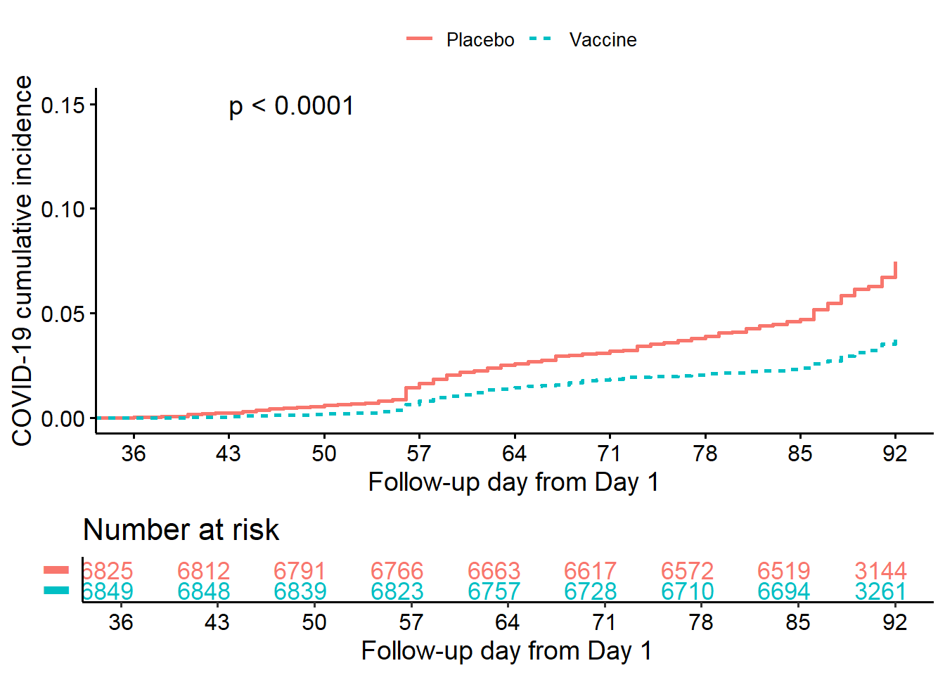

10.7.4.2.2 Stratified by risk category

fit<-survminer::surv_fit(Surv(ttevent3692,event3692)~treatment + riskcov,
             data=subset(ve.ex, mitt_d92=="1"))
cumincr<-ggsurvplot(fit, linetype="strata",
           conf.int=FALSE,pval=FALSE,censor=FALSE,
           risk.table = TRUE,
           risk.table.height = 0.3,
           break.x.by =7,
           xlim=c(36,92),
           fun = "event",
           legend.title ="",
           legend.labs=c("Placebo.Healthy", "Placebo.At_risk",
                         "Vaccine.Healthy","Vaccine.At_risk"),
           tables.col = "strata",
           xlab="Follow-up day from Day 1",
           ylab="COVID-19 cumulative incidence",
           risk.table.y.text = FALSE)
cumincr$plot<-cumincr$plot+
  scale_x_continuous(breaks = c(0,36,43,50,57,64,71,78,85,92))
cumincr$table<-cumincr$table+
  scale_x_continuous(breaks = c(0,36,43,50,57,64,71,78,85,92))
cumincr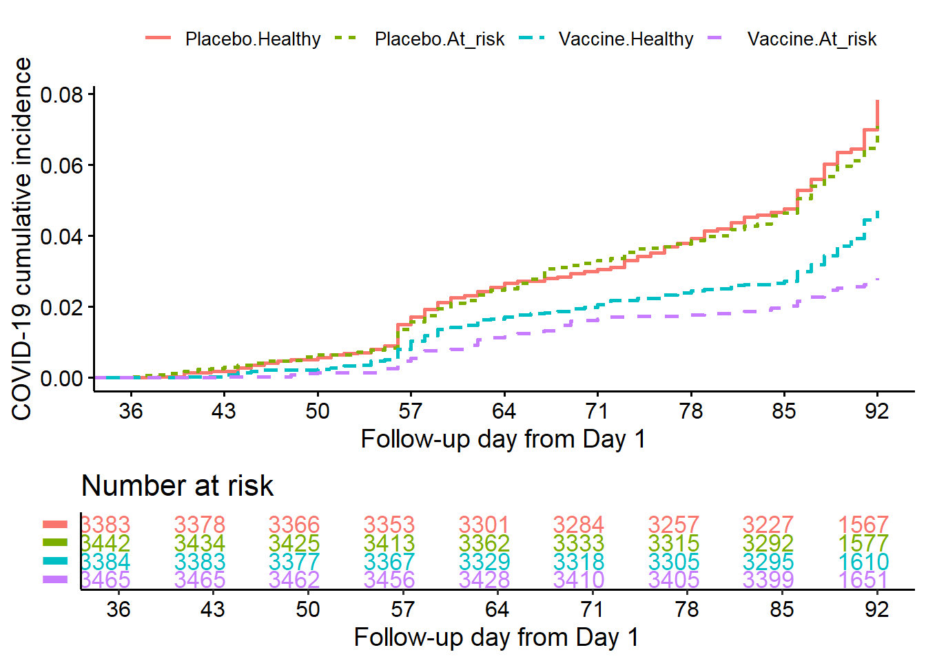

10.7.5 Safety data summary

The codes for safety analysis were adapted from the book R for Clinical Study Reports and Submission (Zhang et al. 2025).

10.7.5.1 Summary of serious adverse events by severity, IP relatedness, death

Summary of safety analysis set:

pop<-ran.ex %>%
  filter(sas == "1") %>%
  count(treatment, name="tot")
pop

##   treatment  tot
## 1   Vaccine 7753
## 2   Placebo 7345

Reformat SAE data and summarize the number and percentage of participants who meet each SAE criteria:

tidy_sae <- sae.ex %>%
  mutate(
    all = sas == "1",
    drug = aerel %in% "1",
    ser = aesev == "3",
    die = aeout == "1"
  ) %>%
  select(usubjid, treatment, all, drug, ser, die) %>%
  pivot_longer(cols = c(all, drug, ser, die))
#summarize the number and percentage of participants who meet each AE criteria.
fmt_num <- function(x, digits, width = digits + 4) {
  formatC(
    x,
    digits = digits,
    format = "f",
    width = width
  )
}
#summarize sae
sum.sae<-tidy_sae %>%
  filter(value == TRUE) %>%
  group_by(treatment, name) %>%
  summarise(n = n_distinct(usubjid))
sum.sae.pop<-merge(sum.sae,pop,by = "treatment", all.x=T)
ana <- sum.sae.pop %>%
  mutate(
    pct = fmt_num(n / tot * 100, digits = 1),
    n = fmt_num(n, digits = 0),
    pct = paste0("(", pct, ")")
  )
ana

##   treatment name    n  tot     pct
## 1   Placebo  all  125 7345 (  1.7)
## 2   Placebo  die    6 7345 (  0.1)
## 3   Placebo drug    7 7345 (  0.1)
## 4   Placebo  ser   31 7345 (  0.4)
## 5   Vaccine  all  130 7753 (  1.7)
## 6   Vaccine  die    9 7753 (  0.1)
## 7   Vaccine drug   10 7753 (  0.1)
## 8   Vaccine  ser   44 7753 (  0.6)

#We prepare reporting-ready dataset for each AE group.
t_sae <- ana %>%
  pivot_wider(
    id_cols = "name",
    names_from = treatment,
    values_from = c(n, pct),
        values_fill = list(
      n = "   0",
      pct = "(  0.0)"
    )
  )%>%
  mutate(Placebo=paste0(n_Placebo," ",pct_Placebo),
         Vaccine=paste0(n_Vaccine," ",pct_Vaccine))%>%
  select(name,Placebo, Vaccine)
t_sae

## # A tibble: 4 × 3
##   name  Placebo        Vaccine       
##   <chr> <chr>          <chr>         
## 1 all   " 125 (  1.7)" " 130 (  1.7)"
## 2 die   "   6 (  0.1)" "   9 (  0.1)"
## 3 drug  "   7 (  0.1)" "  10 (  0.1)"
## 4 ser   "  31 (  0.4)" "  44 (  0.6)"

Prepare reporting-ready datasets and make table:

t_pop <- pop %>%
  mutate(name="sas")%>%
    pivot_wider(
    names_from = treatment,
    values_from = tot
  )%>%
  select(name, Placebo, Vaccine)
t_pop<-lapply(t_pop,as.character)
dp_sae<-bind_rows(t_pop,t_sae)%>%
  mutate(name = factor(
    name,
    c("sas","all", "drug", "ser", "die"),
    c("Participants in SAS",
      "- With one or more SAE",
      "- With IP-related SAE",
      "- With grade 3 SAE",
      "- With SAE with death outcome"
    )
  ))
dp_sae

## # A tibble: 5 × 3
##   name                          Placebo        Vaccine       
##   <fct>                         <chr>          <chr>         
## 1 Participants in SAS           "7345"         "7753"        
## 2 - With one or more SAE        " 125 (  1.7)" " 130 (  1.7)"
## 3 - With SAE with death outcome "   6 (  0.1)" "   9 (  0.1)"
## 4 - With IP-related SAE         "   7 (  0.1)" "  10 (  0.1)"
## 5 - With grade 3 SAE            "  31 (  0.4)" "  44 (  0.6)"

kable(dp_sae, 
      caption = "Summary of serious adverse events",
      col.names = c("Study population",
                            "Placebo n(%)",
                            "Vaccine n(%)"))

Table 10.3: Summary of serious adverse events
Study population	Placebo n(%)	Vaccine n(%)
Participants in SAS	7345	7753
- With one or more SAE	125 ( 1.7)	130 ( 1.7)
- With SAE with death outcome	6 ( 0.1)	9 ( 0.1)
- With IP-related SAE	7 ( 0.1)	10 ( 0.1)
- With grade 3 SAE	31 ( 0.4)	44 ( 0.6)

10.7.5.2 Summary of AE by SOC and PT

Reformat AE data and summarize the number and percentage of participants by SOC:

t1 <- ae.ex %>%
  group_by(treatment, soc) %>%
  summarise(n = fmt_num(n_distinct(usubjid), digits = 0)) %>%
  mutate(pt = soc, order = 0)%>%
  mutate(n=as.numeric(n))
t1.pop<-merge(t1,pop,by = "treatment", all.x=T)
t1.np <- t1.pop %>%
  mutate(
    pct = fmt_num(n / tot * 100, digits = 1),
    n = fmt_num(n, digits = 0),
    pct = paste0("(", pct, ")")
  )

Reformat AE data and summarize the number and percentage of participants by SOC and PT:

t2 <- ae.ex %>%
  group_by(treatment, soc, pt) %>%
  summarise(n = fmt_num(n_distinct(usubjid), digits = 0)) %>%
  mutate(order = 1)%>%
  mutate(n=as.numeric(n))
t2.pop<-left_join(t2, pop, by="treatment")
t2.np <- t2.pop %>%
  mutate(
    pct = fmt_num(n / tot * 100, digits = 1),
    n = fmt_num(n, digits = 0),
    pct = paste0("(", pct, ")")
  )
head(t2.np)

## # A tibble: 6 × 7
## # Groups:   treatment, soc [2]
##   treatment soc                                  pt                          n      order   tot pct   
##   <fct>     <chr>                                <chr>                       <chr>  <dbl> <int> <chr> 
## 1 Vaccine   Blood and lymphatic system disorders Anaemia                     "   1"     1  7753 (  0.…
## 2 Vaccine   Blood and lymphatic system disorders Lymphadenitis               "   3"     1  7753 (  0.…
## 3 Vaccine   Blood and lymphatic system disorders Lymphadenopathy             "   2"     1  7753 (  0.…
## 4 Vaccine   Cardiac disorders                    Acute myocardial infarction "   1"     1  7753 (  0.…
## 5 Vaccine   Cardiac disorders                    Angina pectoris             "   1"     1  7753 (  0.…
## 6 Vaccine   Cardiac disorders                    Angina unstable             "   1"     1  7753 (  0.…

Prepare reporting data for AE and make table:

np_ae<-bind_rows(t1.np, t2.np) %>%
  pivot_wider(
    id_cols = c(soc, order, pt),
    names_from = treatment,
    values_from = c(n,pct),
    values_fill = fmt_num(0, digits = 0)
  ) %>%
  arrange(soc, order, pt) %>%
  mutate(Vaccine=paste0(n_Vaccine," ",pct_Vaccine),
         Placebo=paste0(n_Placebo," ",pct_Placebo)) %>%
  mutate(AE = case_when(
    order==1 ~ paste0("- ",pt),
    TRUE ~ pt)) %>%
  select(AE,Placebo,Vaccine) 
pop.r<-c("Participants in SAS",
         pop$tot[pop$treatment %in% "Placebo"],
         pop$tot[pop$treatment %in% "Vaccine"])
names(pop.r)<-names(np_ae)
np_ae_pop<-bind_rows(pop.r, np_ae)
# Show first 30 rows
kable(head(np_ae_pop,30),
      caption = "Summary of adverse events by SOC & PT",
      col.names = c("Adverse events SOC & PT",
                                   "Placebo n (%)",
                                   "Vaccine n (%)"))

Table 10.4: Summary of adverse events by SOC & PT
Adverse events SOC & PT	Placebo n (%)	Vaccine n (%)
Participants in SAS	7345	7753
Blood and lymphatic system disorders	5 ( 0.1)	6 ( 0.1)
- Anaemia	0 0	1 ( 0.0)
- Iron deficiency anaemia	1 ( 0.0)	0 0
- Lymphadenitis	2 ( 0.0)	3 ( 0.0)
- Lymphadenopathy	2 ( 0.0)	2 ( 0.0)
Cardiac disorders	411 ( 5.6)	453 ( 5.8)
- Acute myocardial infarction	2 ( 0.0)	1 ( 0.0)
- Angina pectoris	2 ( 0.0)	1 ( 0.0)
- Angina unstable	1 ( 0.0)	1 ( 0.0)
- Arrhythmia	2 ( 0.0)	1 ( 0.0)
- Atrial fibrillation	1 ( 0.0)	0 0
- Atrioventricular block complete	0 0	1 ( 0.0)
- Bradycardia	4 ( 0.1)	6 ( 0.1)
- Chest discomfort	11 ( 0.1)	11 ( 0.1)
- Chest pain	8 ( 0.1)	14 ( 0.2)
- Dizziness	19 ( 0.3)	28 ( 0.4)
- Dyspnoea	9 ( 0.1)	4 ( 0.1)
- Heart valve incompetence	0 0	1 ( 0.0)
- Mitral valve incompetence	1 ( 0.0)	0 0
- Myocardial ischaemia	3 ( 0.0)	5 ( 0.1)
- Palpitations	0 0	1 ( 0.0)
- Sinus arrhythmia	0 0	1 ( 0.0)
- Syncope	2 ( 0.0)	1 ( 0.0)
- Tachycardia	352 ( 4.8)	382 ( 4.9)
Congenital, familial and genetic disorders	1 ( 0.0)	0 0
- Atrial septal defect	1 ( 0.0)	0 0
Ear and labyrinth disorders	25 ( 0.3)	43 ( 0.6)
- Ear infection	1 ( 0.0)	2 ( 0.0)
- Ear pain	3 ( 0.0)	4 ( 0.1)

Above are some example codes for analysis and report of example clinical trial data. Ones may apply what have been learnt from previous chapters for further analysis and visualization.

10.8 Reference materials

10.8.1 Books, courses

10.8.2 Other sources

References

Arjyal, Amit, Buddha Basnyat, Ho Thi Nhan, Samir Koirala, Abhishek Giri, Niva Joshi, Mila Shakya, et al. 2016. “Gatifloxacin Versus Ceftriaxone for Uncomplicated Enteric Fever in Nepal: An Open-Label, Two-Centre, Randomised Controlled Trial.” The Lancet Infectious Diseases 16 (May): 535–45. https://doi.org/10.1016/S1473-3099(15)00530-7.

Chow, Shein-Chung, Jun Shao, Hansheng Wang, and Yuliya Lokhnygina. 2017. Sample Size Calculations in Clinical Research: Third Edition. 3rd ed. Chapman; Hall/CRC. https://doi.org/10.1201/9781315183084.

Friedman, Lawrence M., Curt D. Furberg, David L. DeMets, David M. Reboussin, and Christopher B. Granger. 2015. Fundamentals of Clinical Trials. 5th ed. Springer Nature.

Ho, Nhan Thi, Steven G. Hughes, Van Thanh Ta, Lân Trọng Phan, Quyết Đỗ, Thượng Vũ Nguyễn, Anh Thị Văn Phạm, et al. 2024. “Safety, Immunogenicity and Efficacy of the Self-Amplifying mRNA ARCT-154 COVID-19 Vaccine: Pooled Phase 1, 2, 3a and 3b Randomized, Controlled Trials.” Nature Communications 15 (May): 4081. https://doi.org/10.1038/s41467-024-47905-1.

Le, Thuy, Nguyen Van Kinh, Ngo T. K. Cuc, Nguyen L. N. Tung, Nguyen T. Lam, Pham T. T. Thuy, Do D. Cuong, et al. 2017. “A Trial of Itraconazole or Amphotericin b for HIV-Associated Talaromycosis.” New England Journal of Medicine 376 (June): 2329–40. https://doi.org/10.1056/NEJMoa1613306.

Piantadosi, Steven. 2005. “Factorial Designs in Clinical Trials.” In Encyclopedia of Biostatistics. Wiley. https://doi.org/10.1002/0470011815.b2a01025.

Pocock, Stuart J., John J. V. McMurray, and Tim J. Collier. 2015. “Statistical Controversies in Reporting of Clinical Trials.” Journal of the American College of Cardiology 66 (December): 2648–62. https://doi.org/10.1016/j.jacc.2015.10.023.

Qi, Hongchao, and Fang Zhu. 2021. SampleSize4ClinicalTrials: Sample Size Calculation for the Comparison of Means or Proportions in Phase III Clinical Trials. https://CRAN.R-project.org/package=SampleSize4ClinicalTrials.

Zhang, Yilong, Nan Xiao, Keaven Anderson, and Yalin Zhu. 2025. R for Clinical Study Reports and Submission. https://r4csr.org/.