Chapter 2 Introduction to R

Nhan Thi Ho, MD, PhD

2.1 What is R?

R is a free software environment for statistical computing and graphics. To download, install, and learn more, go to R cran (R Core Team 2024b).

2.2 RStudio

RStudio is an integrated development environment (IDE) for R. It includes a console, syntax-highlighting editor that supports direct code execution, as well as tools for plotting, history, debugging and workspace management. To download, install, and learn more, go to RStudio page.

2.3 Rmarkdown

R Markdown is a file format for making dynamic documents with R.
It turns your analyses into high quality REPRODUCIBLE documents, reports, presentations and dashboards (Allaire et al. 2024).
Learn more at Rmarkdown page.

2.4 Base R Example

R comes with a few base packages for base functions.

Example: calculate, generate, summary data:

# Use R as a calculator: 
((2+2)*3)/2

## [1] 6

sqrt(9)

## [1] 3

mean(c(2,4,5,9))

## [1] 5

#Check how to use a function
#?rnorm
#use the function 
data1<- rnorm(n=30,mean=1.5, sd=0.5)
summary(data1)

##    Min. 1st Qu.  Median    Mean 3rd Qu.    Max. 
##  0.6084  1.2695  1.5829  1.5306  1.8650  2.4256

data2<-rnorm(n=35, mean=1.8,sd=1)
summary(data2)

##    Min. 1st Qu.  Median    Mean 3rd Qu.    Max. 
##   0.369   1.345   2.021   1.978   2.426   4.643

Basic statistical test: t-test example:

#?t.test
t.test(x=data1, y=data2, alternative="two.sided",var.equal=FALSE, conf.level=0.95)

## 
##  Welch Two Sample t-test
## 
## data:  data1 and data2
## t = -2.4155, df = 53.351, p-value = 0.01917
## alternative hypothesis: true difference in means is not equal to 0
## 95 percent confidence interval:
##  -0.81885042 -0.07595964
## sample estimates:
## mean of x mean of y 
##  1.530573  1.977978

2.5 Install, load, update R packages

In RStudio: packages>install>packagename From R console: type: install.packages(“packagename”)

Install and load 01 package, which is my R package “metamicrobiomeR” (N. Ho 2020):

#install.packages("metamicrobiomeR")
#load package for use
library("metamicrobiomeR")

Install and load multiple packages

#install multiple packages 
Packages <- c("knitr","rmarkdown","installr","haven","readr","yaml","tidyverse")
#install.packages(Packages)
#load multiple packages
lapply(Packages, library, character.only = TRUE)

Commands useful for updating packages

# download and install newest version of the package
#update.packages()
# shows which packages have updates
#old.packages ()
# looks for new packages that are not already installed
#new.packages ()

Getting help for package, function, data

#help for package
#help(package="metamicrobiomeR")
#help for function
#help("taxa.compare", package="metamicrobiomeR")
#or load package
#library(metamicrobiomeR)
#?taxa.compare
#help for data 
#help(tabsex4, package = "metamicrobiomeR") # display data help page

2.6 Working with R objects

2.6.1 Vector

A vector is a collection of elements:

x<-c(1,3,4,7,8,10)
x

## [1]  1  3  4  7  8 10

a<-c("red","blue","white")
a

## [1] "red"   "blue"  "white"

#creating vector
seq(1,10, by=2)

## [1] 1 3 5 7 9

rep("boring",3)

## [1] "boring" "boring" "boring"

2.6.2 Matrix

A matrix is a 2-dimensional representation of a vector (two-dimensional rectangular data set):

y<-matrix(x, nrow=2)
y

##      [,1] [,2] [,3]
## [1,]    1    4    8
## [2,]    3    7   10

2.6.3 Array

An array is an n dimensional representation of a vector:

z <- array(x, dim = c(1, 3, 2)); z

## , , 1
## 
##      [,1] [,2] [,3]
## [1,]    1    3    4
## 
## , , 2
## 
##      [,1] [,2] [,3]
## [1,]    7    8   10

2.6.4 List

A list is a collection of “bins”, each containing any kind of R object:

mylist <- list(x, y, z, a); mylist

## [[1]]
## [1]  1  3  4  7  8 10
## 
## [[2]]
##      [,1] [,2] [,3]
## [1,]    1    4    8
## [2,]    3    7   10
## 
## [[3]]
## , , 1
## 
##      [,1] [,2] [,3]
## [1,]    1    3    4
## 
## , , 2
## 
##      [,1] [,2] [,3]
## [1,]    7    8   10
## 
## 
## [[4]]
## [1] "red"   "blue"  "white"

2.6.5 Data frame

A data frame is a list in tabular form where each “bin” contains a data vector of the same length. A data frame is the usual tabular data set familiar to epidemiologists. Each row is an record and each column (“bin”) is a field. Both matrix and data.frame are tabular data-types.

All columns in a matrix must have the same data type (numeric, character, etc.) and the same length.
A data frame is more general than a matrix, in that different columns can have different modes (numeric, character, factor, etc.). Just like a table in a database or excel sheet.

smoker <- c("Y", "Y", "N", "N", "Y", "Y", "Y", "N", "Y")
cancer <- c("Y", "N", "N", "Y", "Y", "Y", "N", "N", "Y")
quant<-c(1,2,3,4,5,6,7,8,9)
mydf <- data.frame(smoker, cancer,quant);
mydf[1:4,] # display rows 1 to 4

##   smoker cancer quant
## 1      Y      Y     1
## 2      Y      N     2
## 3      N      N     3
## 4      N      Y     4

2.6.6 Assessing the structure of data objects

data("tabsex4", package="metamicrobiomeR")
str(tabsex4)

## 'data.frame':    701 obs. of  23 variables:
##  $ id                           : chr  "k__bacteria.p__actinobacteria" "k__bacteria.p__bacteroidetes" "k__bacteria.p__firmicutes" "k__bacteria.p__fusobacteria" ...
##  $ Estimate.genderMale          : num  0.2269 -0.1549 -0.056 -0.0648 -0.0887 ...
##  $ Std. Error.genderMale        : num  0.121 0.119 0.104 0.282 0.118 ...
##  $ t value.genderMale           : num  1.874 -1.305 -0.537 -0.23 -0.751 ...
##  $ Pr(>|t|).genderMale          : num  0.0619 0.1931 0.5919 0.8186 0.4532 ...
##  $ Estimate.bfNon_exclusiveBF   : num  -0.3688 0.2557 0.2362 -0.0605 0.3699 ...
##  $ Std. Error.bfNon_exclusiveBF : num  0.139 0.136 0.116 0.364 0.134 ...
##  $ t value.bfNon_exclusiveBF    : num  -2.647 1.887 2.035 -0.166 2.764 ...
##  $ Pr(>|t|).bfNon_exclusiveBF   : num  0.00857 0.0602 0.04276 0.86812 0.00606 ...
##  $ Estimate.bfNo_BF             : num  -1.329 0.135 0.356 -0.403 1.153 ...
##  $ Std. Error.bfNo_BF           : num  0.412 0.499 0.392 1.083 0.407 ...
##  $ t value.bfNo_BF              : num  -3.223 0.27 0.908 -0.372 2.834 ...
##  $ Pr(>|t|).bfNo_BF             : num  0.00141 0.7873 0.36478 0.7103 0.0049 ...
##  $ Estimate.age.sample          : num  0.1251 0.0242 0.0115 0.0285 -0.1348 ...
##  $ Std. Error.age.sample        : num  0.0377 0.0367 0.0319 0.0857 0.038 ...
##  $ t value.age.sample           : num  3.318 0.66 0.359 0.333 -3.549 ...
##  $ Pr(>|t|).age.sample          : num  0.001022 0.510068 0.719525 0.73934 0.000448 ...
##  $ pval.adjust.genderMale       : num  0.48 0.899 0.961 0.961 0.961 ...
##  $ pval.adjust.bfNon_exclusiveBF: num  0.059 0.2333 0.1767 0.9976 0.0448 ...
##  $ pval.adjust.bfNo_BF          : num  0.0219 1 1 1 0.0468 ...
##  $ pval.adjust.sample           : num  0.00786 0.82595 0.85375 0.85375 0.00505 ...
##  $ study                        : chr  "Subramanian et al 2014 (Bangladesh)" "Subramanian et al 2014 (Bangladesh)" "Subramanian et al 2014 (Bangladesh)" "Subramanian et al 2014 (Bangladesh)" ...
##  $ pop                          : chr  "Bangladesh" "Bangladesh" "Bangladesh" "Bangladesh" ...

2.6.7 Useful functions to assess R objects

Function	Returns
str	summary of data object structure
attributes	list with data object attributes
mode	mode of object
typeof	type of object; similar to mode but includes double and integer, if applicable
length	length of object
class	class of object, if it exists
dim	vector with object dimensions, if applicable
nrow	number of rows, if applicable
ncol
dimnames	list containing vectors of names for each dimension, if applicable
rownames	vector of row names of a matrix-like object
colnames	vector of column names of a matrix-like object
names	vector of names for the list (for a data frame returns field names)
row.names	vector of row names for a data frame

2.6.8 Understanding vectors

Operation of vectors

#Generate vector
x1 <- 5; y1 <- c(10, 20, 30)
x2 <- c(5, 5, 5); y2 <- c(10, 20, 30)
x1 * y1

## [1]  50 100 150

x2 * y2

## [1]  50 100 150

2.6.8.1 Boolean queries and subsetting of vectors

lecturer <- c('Nhan', 'Hien', 'Phuong', 'Tien', 'Duy')
lecturer

## [1] "Nhan"   "Hien"   "Phuong" "Tien"   "Duy"

ms.ages <- c(41, 39, 33, 26, 25)
ms.ages

## [1] 41 39 33 26 25

ms.ages >= 30 # logical vector for lecturers with ages >=30

## [1]  TRUE  TRUE  TRUE FALSE FALSE

thirtysomething <- (ms.ages >= 30) & (ms.ages < 40)
lecturer[thirtysomething] # indexing using logical

## [1] "Hien"   "Phuong"

#naming vector
names(ms.ages)<-lecturer
ms.ages

##   Nhan   Hien Phuong   Tien    Duy 
##     41     39     33     26     25

2.6.8.2 Operations on single vectors

Some operations on single vectors.

Function	Description	Function	Description
sum	summation	rev	reverse order
cumsum	cumulative	sum	order order
diff	x[i+1]-x[i]	sort	sort
prod	product	rank	rank
cumprod	cumulative product	sample	random sample
mean	mean	quantile	percentile
median	median	var	variance, covariance
min	minimum	sd	standard deviation
max	maximum	table	tabulate character vector
range	range	xtabs	tabulate factor vector

2.7 Managing biomedical data in R

2.7.1 Entering data

Enter simple data frame

subjname <- c('Lop', 'Chung', 'Minh')
subjno <- 1:length(subjname)
age <- c(34, 56, 56)
sex <- c('Male', 'Male', 'Female')
dat <- data.frame(subjno, subjname, age, sex); dat

##   subjno subjname age    sex
## 1      1      Lop  34   Male
## 2      2    Chung  56   Male
## 3      3     Minh  56 Female

2.7.2 Importing data from a file

From local: (Example data of Bangladeshi children (Subramanian et al. 2014)).

#your path to dataset
fdir1<-"./metamicrobiomeR-master/inst/extdata/QIIME_outputs/Bangladesh/"
#Read in text file 
dat1<-read.delim(paste(fdir1,"Subramanian_et_al_mapping_file.txt",sep=""),header=T,sep ="")
#Or simply: 
#dat1<-read.delim("./metamicrobiomeR-master/inst/extdata/QIIME_outputs/Bangladesh/Subramanian_et_al_mapping_file.txt",header=T,sep ="")

From URL:

#Read in csv file
test.csv <- read.csv("https://stats.idre.ucla.edu/wp-content/uploads/2016/02/test-1.csv", header=T)

2.7.3 Some other data import functions

Data import with “rio” makes our life much easier! All you need is import()!

#install.packages("rio")
#install.packages(c('csvy', 'feather', 'fst', 'hexView', 'readODS', 'rmatio'))
library(rio)
test1<-import(paste(fdir1,"Subramanian_et_al_mapping_file.txt",sep=""))

Import excel files with multiple sheets:

#import always  get only 1 dataframe
test<-import(paste(fdir1,"nature13421-s2.xlsx",sep=""),sheet=1,skip=1) 
 
#Import multiple sheets of an excel file and create a list of dataframes
list1<-import_list(paste(fdir1,"nature13421-s2.xlsx",sep=""))
#str(list1)
#View(list1[[1]])

Multiple files from a directory

#Sys.glob() allows you to find files using a regular expression
dir1<-Sys.glob(paste(fdir1,"alpha_div_collated/*.txt",sep=""))
list2<-import_list(dir1)
#str(list2)

2.7.4 Exporting data

#save one dataframe as an csv file
#write.csv(dat1,file=paste(fdir1,"dat1.csv",sep=""),row.names = F)

#save multiple data objects
#save(dat1,list1,list2, file=paste(fdir1,"manyfile.rda",sep=""))

#load saved files
#print(load(paste(fdir1,"manyfile.rda",sep="")))

2.7.5 Basic data manipulation with “tidyverse”

“tidyverse” includes a collection of open source packages for the R programming language that share similar design philosophy, grammar, and data structures” for tidy data (Wickham 2023b).

2.7.5.1 Pipes

Pipes take the output of a command, and feed it as the input of another command.

library(tidyverse)
#pipe from library(magrittr), loaded along with other packages
9 %>% sqrt %>% `+`(8)

## [1] 11

2.7.5.2 Subset data

Subset data by column and row

dat2a<-test %>%
  slice(1:50) %>%
  select(-starts_with("..."))

2.7.5.3 Change column names

#change column name
colnames(dat2a)<-tolower(colnames(dat2a))
oldname<-colnames(dat2a)
newname<-c("child.id",
           "family.id",
           "cohort",
           "gender",
           "zygosity",
           "whz","waz","haz",
           "age.first.fe",
           "age.last.fe", 
           "no.fe.sam",
           "sam.int.mean",
           "month.ebf",
           "age.first.solid",
           "no.diarhea.yr",
           "pc.days.diarrhea",
           "frac.sam.atb.7day",
           "set")
dat2a<-dat2a %>% rename_at(vars(oldname), ~newname)
#colnames(dat2a)

2.7.5.4 Subset data by row

dat.tw<-dat2a %>% filter(cohort == "Healthy Twins & Triplets")
#more filter 
dat.tw<-dat2a %>% 
  filter(cohort == "Healthy Twins & Triplets")%>%
  filter(!is.na(zygosity))%>%
  filter(between(whz,-1,1))
#or
dat.tw<-dat2a %>% 
  filter(cohort == "Healthy Twins & Triplets" & 
           !is.na(zygosity) & 
           between(whz,-1,1))

2.7.5.5 Select columns

#Base R
#Select by position (cautious!)
subdat<-dat2a[,c(1,4:6)]
#or select specific column names
subdat<-dat2a[,c("child.id","gender","zygosity","whz")]

#pipes and select()
subdat<-dat2a %>% select(c(1,4:6))
subdat<-dat2a %>% select(child.id,gender,zygosity,whz)

2.7.5.6 Discard columns

#Base R
subdat<-dat2a[,-c(1,4:6)]
subdat<-dat2a[,colnames(dat2a)[!colnames(dat2a) %in% c("child.id","gender","zygosity","whz")]]
#or
subdat<-dat2a %>% select(-c(1,4:6))
subdat<-dat2a %>% select(-c("child.id","gender","zygosity","whz"))

2.7.5.7 Rename columns

#Base R
#colnames(dat2a)[colnames(dat2a)=="child.id"]<-"childid"
#with tidyverse
dat2a<-dat2a %>% select(childid=child.id, everything())
dat2a<-dat2a %>% rename(child.id=childid)

2.7.5.8 Editting data

#initial look at data 
summary(dat2a)

##    child.id          family.id            cohort             gender            zygosity        
##  Length:50          Length:50          Length:50          Length:50          Length:50         
##  Class :character   Class :character   Class :character   Class :character   Class :character  
##  Mode  :character   Mode  :character   Mode  :character   Mode  :character   Mode  :character  
##                                                                                                
##                                                                                                
##                                                                                                
##       whz                waz               haz           age.first.fe    age.last.fe   
##  Min.   :-1.73842   Min.   :-3.7555   Min.   :-4.6586   Min.   : 1.00   Min.   :286.0  
##  1st Qu.:-0.88598   1st Qu.:-2.6037   1st Qu.:-3.4314   1st Qu.: 5.00   1st Qu.:455.0  
##  Median :-0.47063   Median :-1.5116   Median :-1.5749   Median : 6.00   Median :700.5  
##  Mean   :-0.42223   Mean   :-1.5148   Mean   :-1.8570   Mean   : 9.78   Mean   :600.6  
##  3rd Qu.:-0.03458   3rd Qu.:-0.7189   3rd Qu.:-0.7189   3rd Qu.: 9.75   3rd Qu.:706.0  
##  Max.   : 1.20133   Max.   : 1.6698   Max.   : 1.6698   Max.   :37.00   Max.   :738.0  
##    no.fe.sam      sam.int.mean     month.ebf      age.first.solid no.diarhea.yr   pc.days.diarrhea
##  Min.   : 9.00   Min.   :22.56   Min.   :0.0000   Min.   :1.216   Min.   :0.000   Min.   : 0.000  
##  1st Qu.:18.00   1st Qu.:28.29   1st Qu.:0.1971   1st Qu.:4.920   1st Qu.:1.271   1st Qu.: 1.163  
##  Median :21.00   Median :30.48   Median :1.0348   Median :6.932   Median :2.916   Median : 2.742  
##  Mean   :19.92   Mean   :31.34   Mean   :2.0716   Mean   :6.690   Mean   :2.971   Mean   : 3.125  
##  3rd Qu.:23.00   3rd Qu.:33.27   3rd Qu.:3.2523   3rd Qu.:8.361   3rd Qu.:4.054   3rd Qu.: 4.314  
##  Max.   :26.00   Max.   :42.29   Max.   :7.3260   Max.   :9.790   Max.   :8.814   Max.   :10.826  
##  frac.sam.atb.7day     set           
##  Min.   :0.00000   Length:50         
##  1st Qu.:0.08083   Class :character  
##  Median :0.11882   Mode  :character  
##  Mean   :0.18328                     
##  3rd Qu.:0.28373                     
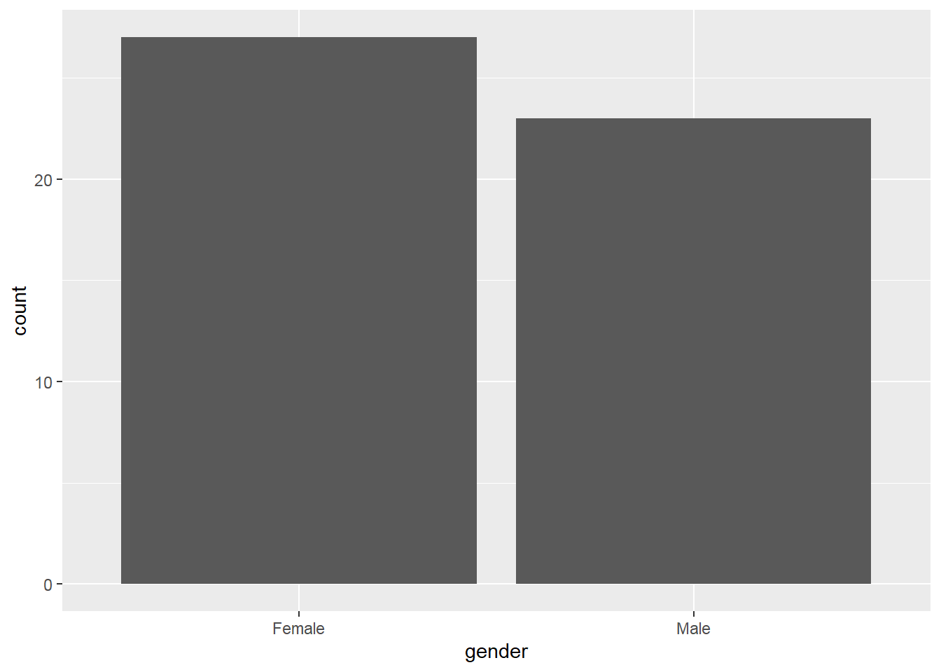
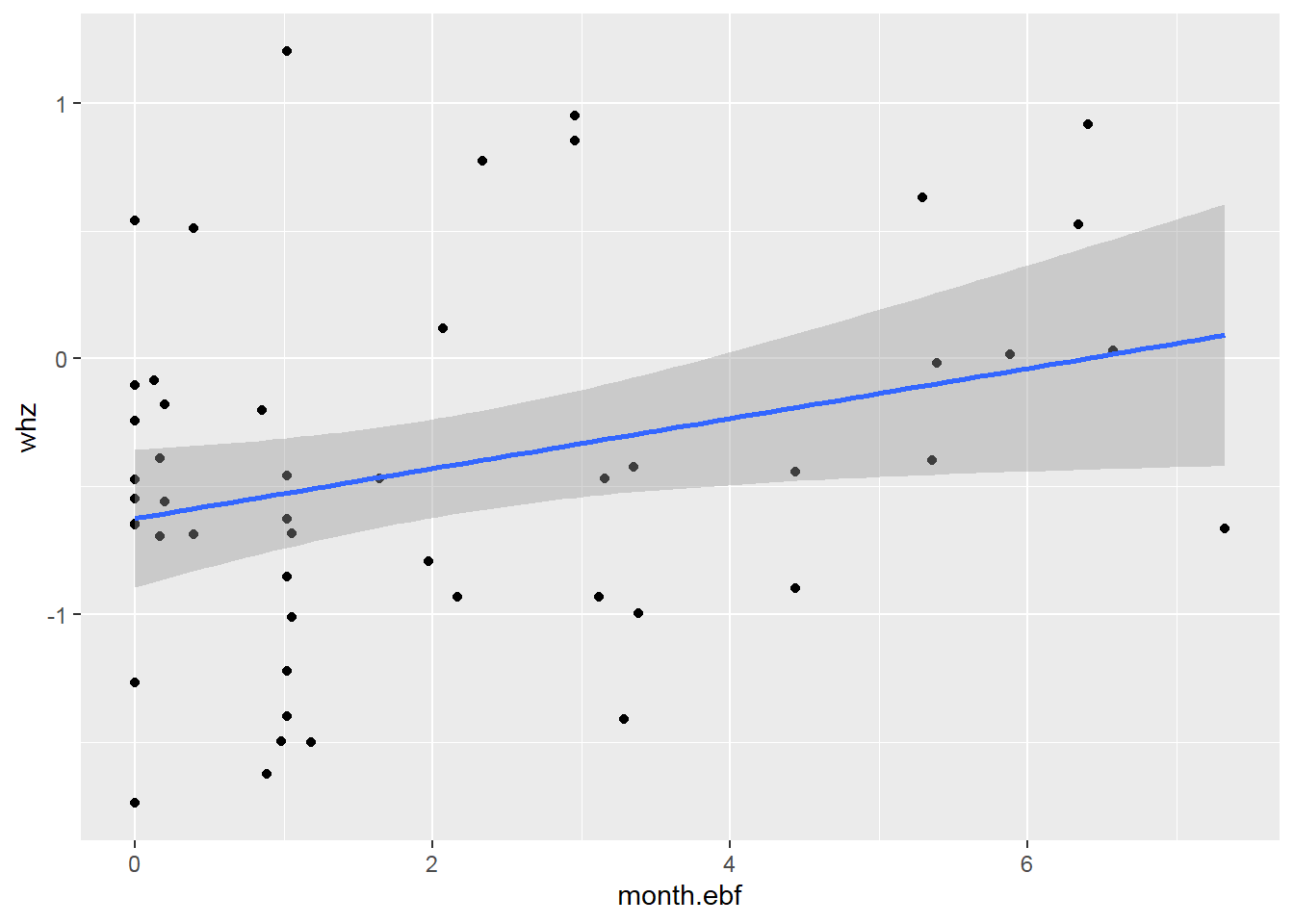
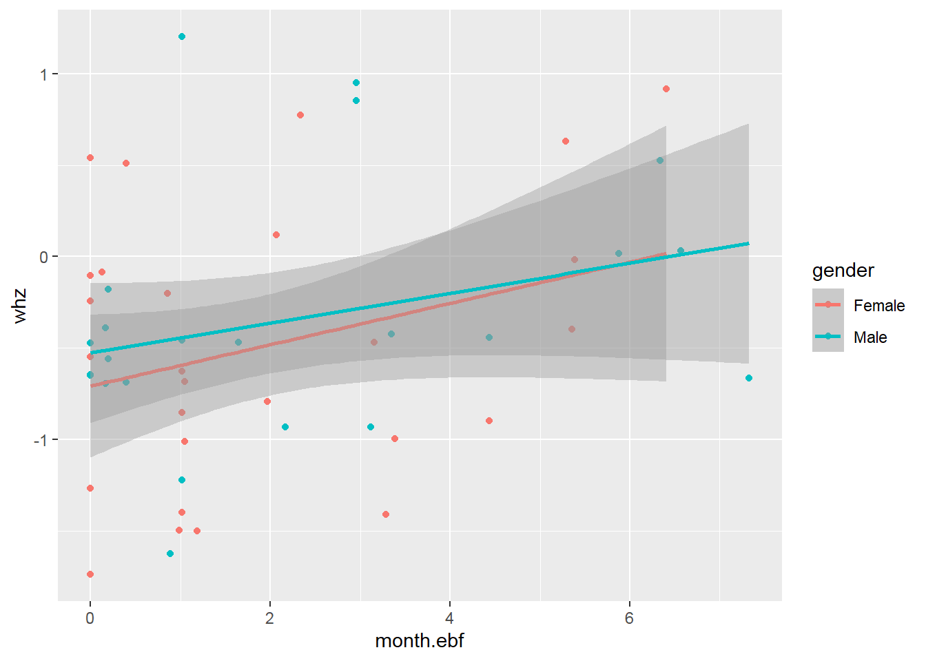
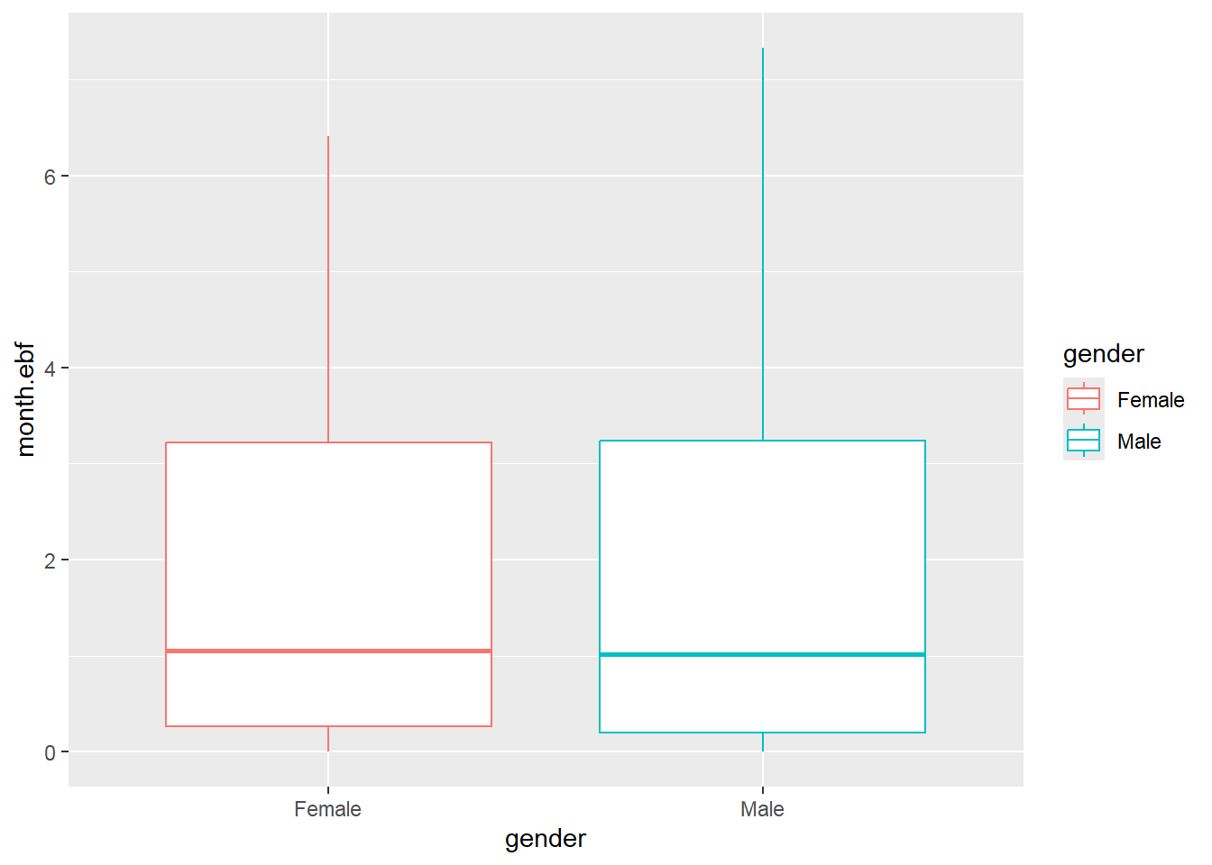
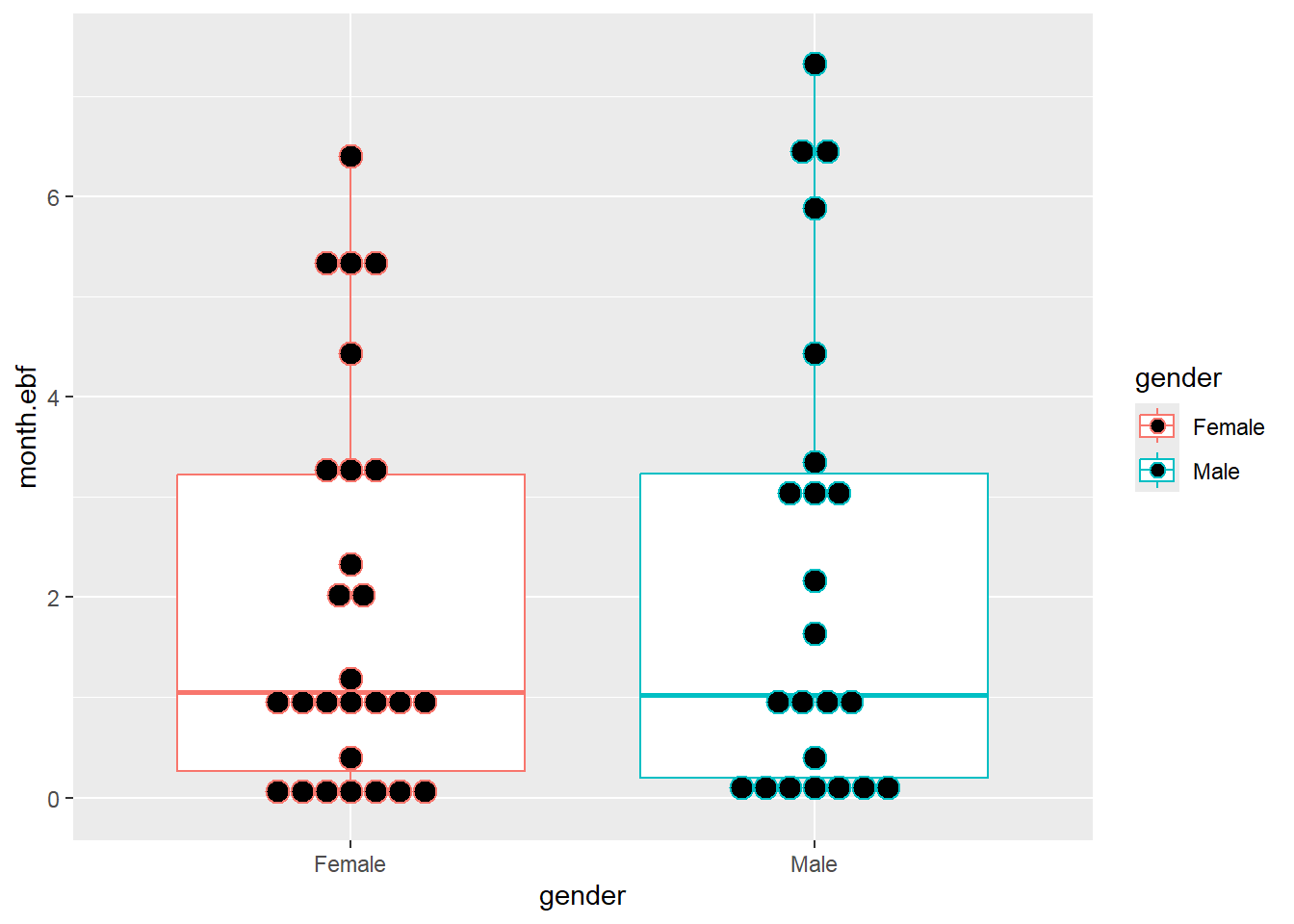
##  Max.   :0.50000

dat2a<-dat2a %>%
  mutate(zygosity=replace(zygosity,zygosity=="NA","singleton")) %>%
  mutate(zygosity=replace(zygosity,zygosity=="not tested",NA))

2.8 Basic data visualization

Below are some examples of basic data visualization with ggplot2 .

2.8.1 Barplot

library(ggthemes)
ggplot(dat2a,aes(gender))+
  geom_bar()

2.8.2 Histogram

ggplot(dat2a,aes(whz))+
  geom_histogram(bins=10)

2.8.2.1 Plot by group

ggplot(dat2a,aes(whz,fill=gender))+
  geom_histogram(bins=10,alpha=0.5, position="identity")

2.8.3 Density

ggplot(dat2a, aes(whz)) +
  geom_density()

2.8.3.1 Plot by group

ggplot(dat2a, aes(whz, fill=gender)) +
  geom_density(alpha=0.5)

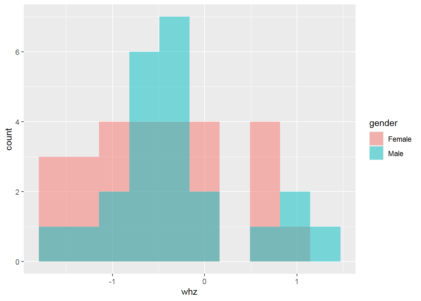
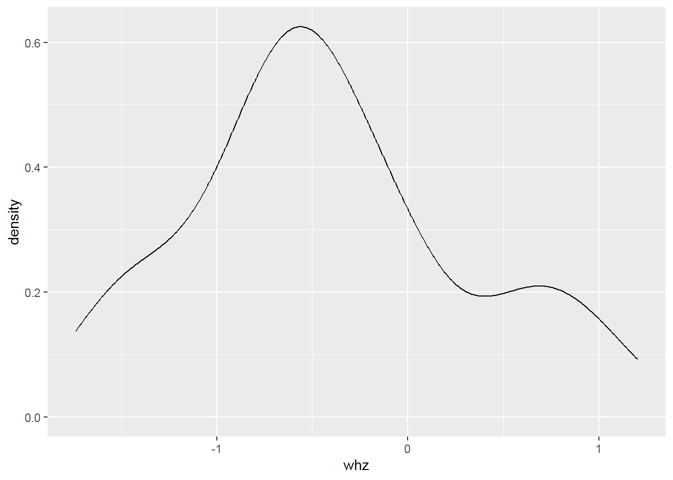
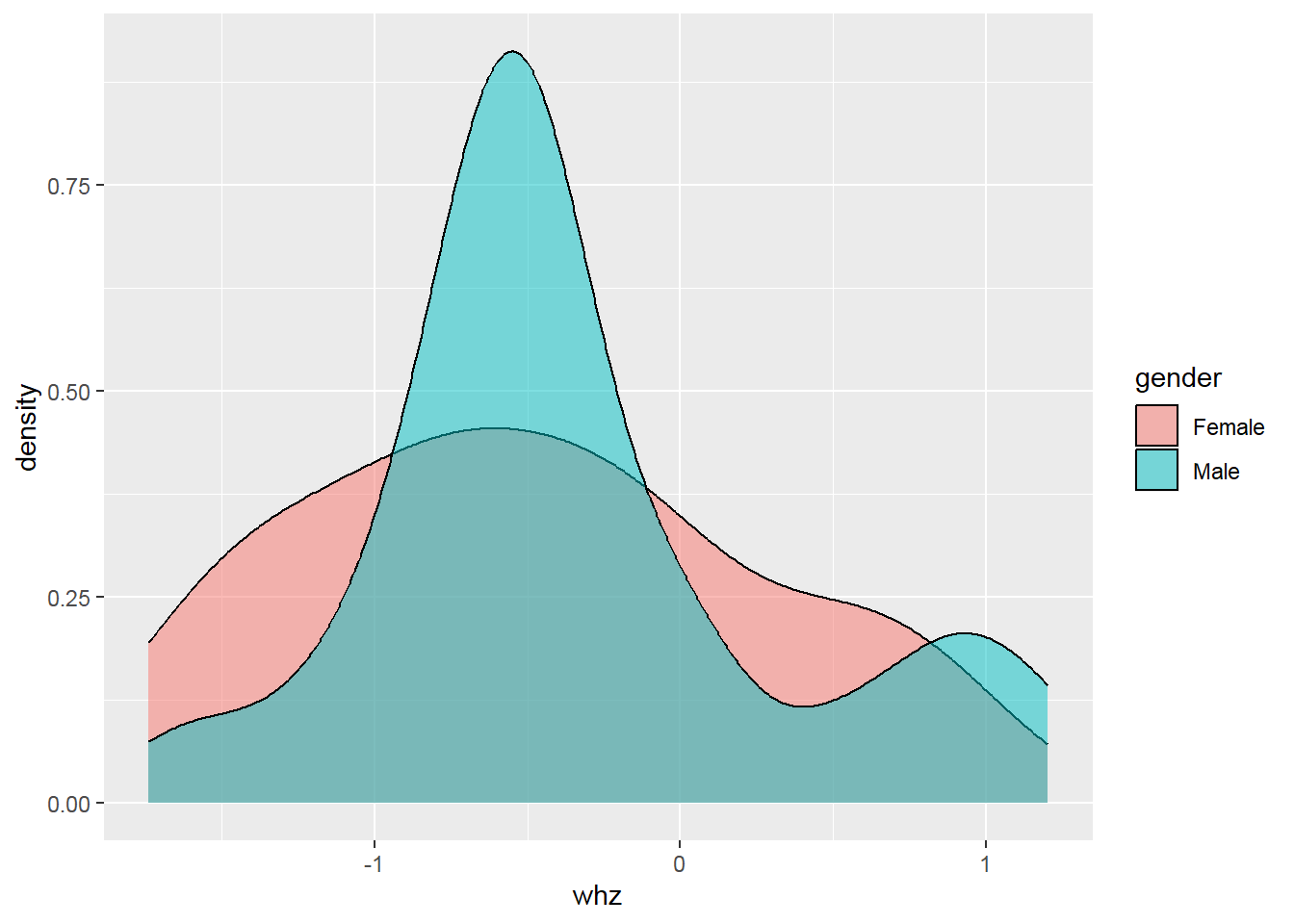
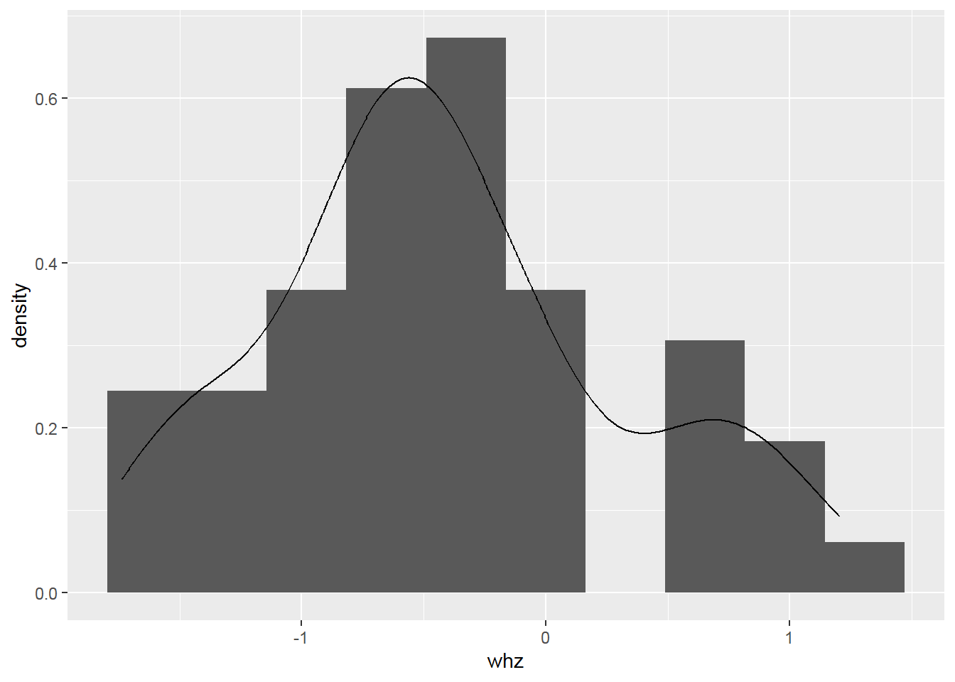
2.8.4 Histogram with density

ggplot(dat2a,aes(whz))+
  geom_histogram(bins=10)+
  geom_density()

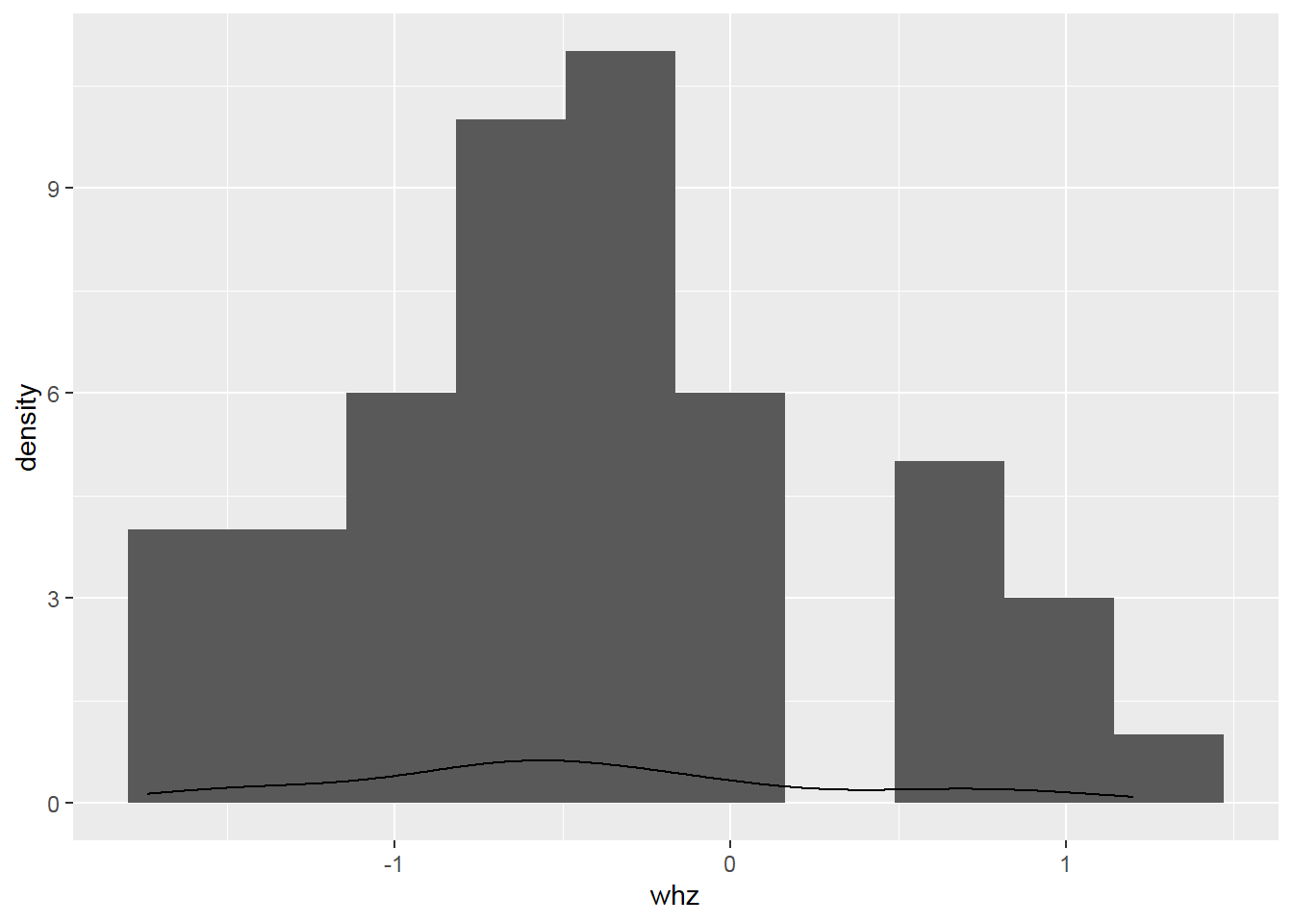
Something goes wrong! => Create a histogram with a density scale using the computed variable ..density..:

ggplot(dat2a)+
  geom_histogram(aes(x=whz,y=..density..),bins=10)+
  geom_density(aes(whz))

2.8.4.1 By group

ggplot(dat2a)+
  geom_histogram(aes(x=whz,y=..density..,fill = gender),bins=10, position="identity",alpha=0.5)+
  geom_density(aes(whz,color=gender))

2.8.5 Scatter plot

ggplot(dat2a,aes(x=month.ebf, y=whz)) +
  geom_point()

2.8.5.1 With regression line

ggplot(dat2a,aes(x=month.ebf, y=whz)) +
  geom_point()+
  stat_smooth(method = 'glm')

2.8.5.2 By group

ggplot(dat2a,aes(x=month.ebf, y=whz,color=gender)) +
  geom_point()+
  stat_smooth(method = 'glm')

2.8.6 Boxplot

ggplot(dat2a,aes(x=gender, y=month.ebf, color=gender)) +
  geom_boxplot()

2.8.6.1 Box plot with dots

ggplot(dat2a,aes(x=gender, y=month.ebf, color=gender)) +
  geom_boxplot()+ 
  geom_dotplot(binaxis='y', stackdir='center', dotsize=1)

2.8.7 Pie Charts

dat2a %>% 
  group_by(gender) %>%
  summarise(count=n()) %>%
ggplot(aes(x="",y=count,fill=gender)) +
  geom_bar(stat = "identity") +
  coord_polar("y", start = 0)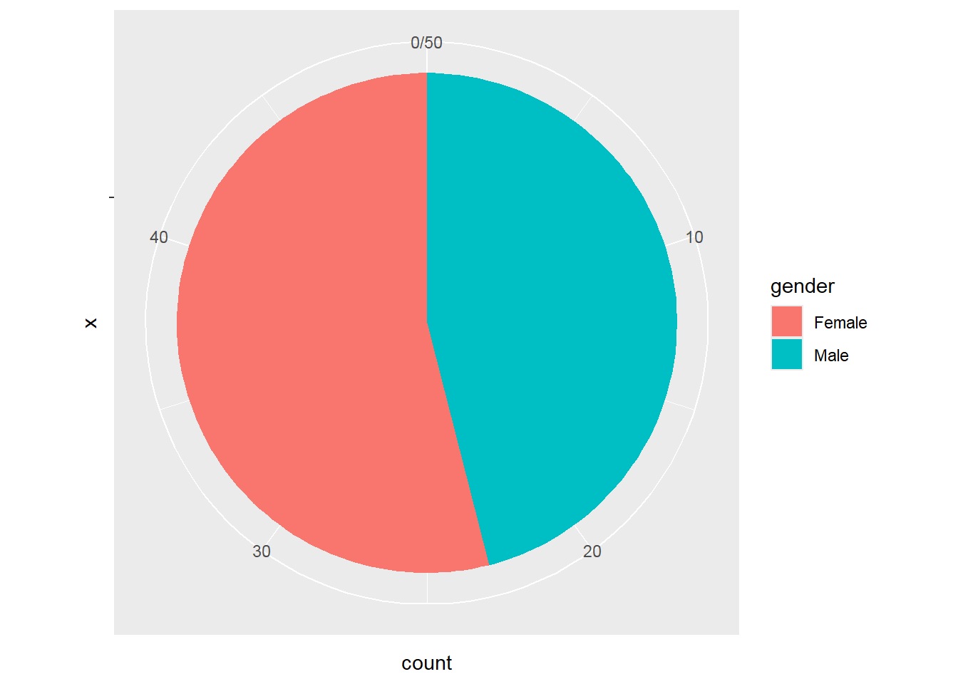

2.8.8 More data visualization

Please see Chapter “Data visualization” of this book.

2.8.8.1 Some useful resources

2.9 Summary statistics

2.9.1 Basic descriptive summary functions

# Summary of variable month.ebf 
dat2a %>% 
  summarise(
    count = n(),
    mean = mean(month.ebf, na.rm = TRUE),
    sd = sd(month.ebf, na.rm = TRUE),
    median = median(month.ebf, na.rm = TRUE),
    IQR = IQR(month.ebf, na.rm = TRUE))

##   count     mean       sd   median      IQR
## 1    50 2.071644 2.154823 1.034836 3.055231

2.9.1.1 Summary by group

# Summary of month.ebf by cohort
dat2a %>% group_by(cohort) %>%
  summarise(
    count = n(),
    mean = mean(month.ebf, na.rm = TRUE),
    sd = sd(month.ebf, na.rm = TRUE),
    median = median(month.ebf, na.rm = TRUE),
    IQR = IQR(month.ebf, na.rm = TRUE))

## # A tibble: 2 × 6
##   cohort                         count  mean    sd median   IQR
##   <chr>                          <int> <dbl> <dbl>  <dbl> <dbl>
## 1 Healthy Singleton Birth Cohort    25 3.45  2.24   3.29   3.71
## 2 Healthy Twins & Triplets          25 0.694 0.706  0.854  1.02

2.9.1.2 Summary by subgroup of another group

dat2a %>% filter(cohort == "Healthy Twins & Triplets") %>%
  group_by(gender) %>%
  summarise(
    count = n(),
    mean = mean(month.ebf, na.rm = TRUE),
    sd = sd(month.ebf, na.rm = TRUE),
    median = median(month.ebf, na.rm = TRUE),
    IQR = IQR(month.ebf, na.rm = TRUE))

## # A tibble: 2 × 6
##   gender count  mean    sd median   IQR
##   <chr>  <int> <dbl> <dbl>  <dbl> <dbl>
## 1 Female    18 0.772 0.770  0.920 1.04 
## 2 Male       7 0.493 0.498  0.197 0.920

2.9.1.3 More filter

dat2a %>% filter(cohort == "Healthy Twins & Triplets") %>%
  filter(!is.na(zygosity)) %>%
  group_by(gender) %>%
  summarise(
    count = n(),
    mean = mean(month.ebf, na.rm = TRUE),
    sd = sd(month.ebf, na.rm = TRUE),
    median = median(month.ebf, na.rm = TRUE),
    IQR = IQR(month.ebf, na.rm = TRUE))

## # A tibble: 2 × 6
##   gender count  mean    sd median   IQR
##   <chr>  <int> <dbl> <dbl>  <dbl> <dbl>
## 1 Female    16 0.749 0.816  0.690 1.03 
## 2 Male       7 0.493 0.498  0.197 0.920

2.9.2 Basic statistical test examples

2.9.2.1 Continuous variables: parametric

#t-test
summary(dat2a$whz)

##     Min.  1st Qu.   Median     Mean  3rd Qu.     Max. 
## -1.73842 -0.88598 -0.47063 -0.42223 -0.03458  1.20133

hist(dat2a$whz)

t.test(whz~gender, data=dat2a)

## 
##  Welch Two Sample t-test
## 
## data:  whz by gender
## t = -0.7285, df = 47.802, p-value = 0.4699
## alternative hypothesis: true difference in means between group Female and group Male is not equal to 0
## 95 percent confidence interval:
##  -0.5572199  0.2608470
## sample estimates:
## mean in group Female   mean in group Male 
##           -0.4903957           -0.3422092

2.9.2.2 Continuous variables: non-parametric

#Kruskal-Wallis 
summary(dat2a$month.ebf)

##    Min. 1st Qu.  Median    Mean 3rd Qu.    Max. 
##  0.0000  0.1971  1.0348  2.0716  3.2523  7.3260

hist(dat2a$month.ebf)

kruskal.test(month.ebf ~ gender, data = dat2a)

## 
##  Kruskal-Wallis rank sum test
## 
## data:  month.ebf by gender
## Kruskal-Wallis chi-squared = 0.12372, df = 1, p-value = 0.725

#wilcox.test
wilcox.test(month.ebf ~ gender, data = dat2a)

## 
##  Wilcoxon rank sum test with continuity correction
## 
## data:  month.ebf by gender
## W = 292.5, p-value = 0.7324
## alternative hypothesis: true location shift is not equal to 0

2.9.2.3 Categorical variables

#Chi-square
table(dat2a$cohort,dat2a$gender)

##                                 
##                                  Female Male
##   Healthy Singleton Birth Cohort      9   16
##   Healthy Twins & Triplets           18    7

chisq.test(dat2a$cohort,dat2a$gender)

## 
##  Pearson's Chi-squared test with Yates' continuity correction
## 
## data:  dat2a$cohort and dat2a$gender
## X-squared = 5.153, df = 1, p-value = 0.02321

#Fisher 
fisher.test(dat2a$cohort,dat2a$gender)

## 
##  Fisher's Exact Test for Count Data
## 
## data:  dat2a$cohort and dat2a$gender
## p-value = 0.02224
## alternative hypothesis: true odds ratio is not equal to 1
## 95 percent confidence interval:
##  0.05544835 0.83324786
## sample estimates:
## odds ratio 
##  0.2261644

2.9.3 Summary statistic table

2.9.3.1 Packages for quick, nice summary table

The “arsenal” package provides handy R functions for large-scale statistical summaries (Heinzen et al. 2021).

#install.packages(c("Deducer","arsenal","qwraps2","table1","tangram","purrrlyr","Gmisc")) 
library(arsenal)
ca.vars<-c("cohort","gender","zygosity")
co.vars<-c("whz", "waz", "haz","age.first.fe","age.last.fe","no.fe.sam","sam.int.mean",
        "month.ebf","age.first.solid","no.diarhea.yr","pc.days.diarrhea","frac.sam.atb.7day")
varuse<-c(co.vars,ca.vars[!ca.vars %in% "cohort"])
mylabels <-as.list(varuse)
names(mylabels)<-varuse
tab1 <- tableby(as.formula(paste("cohort",paste(varuse,collapse="+"),sep="~")), 
                data = dat2a)
kable(summary(tab1,
        labelTranslations = mylabels, 
        text=TRUE))

	Healthy Singleton Birth Cohort (N=25)	Healthy Twins & Triplets (N=25)	Total (N=50)	p value
whz				0.683
- Mean (SD)	-0.380 (0.727)	-0.464 (0.724)	-0.422 (0.719)
- Range	-1.623 - 0.949	-1.738 - 1.201	-1.738 - 1.201
waz				< 0.001
- Mean (SD)	-0.483 (0.806)	-2.546 (0.561)	-1.515 (1.248)
- Range	-1.741 - 1.670	-3.755 - -1.392	-3.755 - 1.670
haz				< 0.001
- Mean (SD)	-0.483 (0.806)	-3.231 (0.956)	-1.857 (1.641)
- Range	-1.741 - 1.670	-4.659 - -1.412	-4.659 - 1.670
age.first.fe				0.008
- Mean (SD)	6.360 (2.782)	13.200 (12.124)	9.780 (9.366)
- Range	3.000 - 15.000	1.000 - 37.000	1.000 - 37.000
age.last.fe				< 0.001
- Mean (SD)	710.400 (12.430)	490.880 (152.553)	600.640 (154.167)
- Range	700.000 - 738.000	286.000 - 730.000	286.000 - 738.000
no.fe.sam				0.001
- Mean (SD)	21.920 (2.019)	17.920 (5.338)	19.920 (4.476)
- Range	18.000 - 24.000	9.000 - 26.000	9.000 - 26.000
sam.int.mean				< 0.001
- Mean (SD)	34.003 (3.813)	28.677 (3.090)	31.340 (4.363)
- Range	30.087 - 42.294	22.562 - 35.000	22.562 - 42.294
month.ebf				< 0.001
- Mean (SD)	3.449 (2.242)	0.694 (0.706)	2.072 (2.155)
- Range	0.000 - 7.326	0.000 - 2.332	0.000 - 7.326
age.first.solid				0.254
- Mean (SD)	6.352 (2.236)	7.028 (1.884)	6.690 (2.074)
- Range	1.216 - 9.790	3.088 - 9.396	1.216 - 9.790
no.diarhea.yr				< 0.001
- Mean (SD)	4.278 (2.135)	1.664 (1.345)	2.971 (2.205)
- Range	0.520 - 8.814	0.000 - 4.986	0.000 - 8.814
pc.days.diarrhea				0.007
- Mean (SD)	4.090 (2.223)	2.159 (2.601)	3.125 (2.585)
- Range	0.142 - 10.826	0.000 - 9.563	0.000 - 10.826
frac.sam.atb.7day				0.070
- Mean (SD)	0.219 (0.145)	0.148 (0.125)	0.183 (0.139)
- Range	0.000 - 0.500	0.000 - 0.462	0.000 - 0.500
gender				0.011
- Female	9 (36.0%)	18 (72.0%)	27 (54.0%)
- Male	16 (64.0%)	7 (28.0%)	23 (46.0%)
zygosity				< 0.001
- N-Miss	0	2	2
- DZ	0 (0.0%)	12 (52.2%)	12 (25.0%)
- Fraternal co-twin in set of triplets	0 (0.0%)	1 (4.3%)	1 (2.1%)
- MZ	0 (0.0%)	8 (34.8%)	8 (16.7%)
- MZ co-twin in set of triplets	0 (0.0%)	2 (8.7%)	2 (4.2%)
- singleton	25 (100.0%)	0 (0.0%)	25 (52.1%)

#Feel free to try other packages!

2.9.3.2 More comprehensive table (control)

my_controls <- tableby.control(
  test = T,
  total = T,
  numeric.test = "kwt", cat.test = "fe",
  numeric.stats = c("meansd", "medianq1q3", "range", "Nmiss2"),
  cat.stats = c("countpct", "Nmiss2"),
  stats.labels = list(
    meansd = "Mean (SD)",
    medianq1q3 = "Median (Q1, Q3)",
    range = "Min - Max",
    Nmiss2 = "Missing"
  )
)
tab2 <- tableby(as.formula(paste("cohort",paste(varuse,collapse="+"),sep="~")),data = dat2a,
                control = my_controls)
kable(summary(tab2,labelTranslations = mylabels, text=TRUE))

	Healthy Singleton Birth Cohort (N=25)	Healthy Twins & Triplets (N=25)	Total (N=50)	p value
whz				0.705
- Mean (SD)	-0.380 (0.727)	-0.464 (0.724)	-0.422 (0.719)
- Median (Q1, Q3)	-0.468 (-0.897, 0.015)	-0.560 (-0.853, -0.104)	-0.471 (-0.886, -0.035)
- Min - Max	-1.623 - 0.949	-1.738 - 1.201	-1.738 - 1.201
- Missing	0	0	0
waz				< 0.001
- Mean (SD)	-0.483 (0.806)	-2.546 (0.561)	-1.515 (1.248)
- Median (Q1, Q3)	-0.706 (-1.031, -0.030)	-2.606 (-2.879, -2.295)	-1.512 (-2.604, -0.719)
- Min - Max	-1.741 - 1.670	-3.755 - -1.392	-3.755 - 1.670
- Missing	0	0	0
haz				< 0.001
- Mean (SD)	-0.483 (0.806)	-3.231 (0.956)	-1.857 (1.641)
- Median (Q1, Q3)	-0.706 (-1.031, -0.030)	-3.437 (-4.032, -2.551)	-1.575 (-3.431, -0.719)
- Min - Max	-1.741 - 1.670	-4.659 - -1.412	-4.659 - 1.670
- Missing	0	0	0
age.first.fe				0.077
- Mean (SD)	6.360 (2.782)	13.200 (12.124)	9.780 (9.366)
- Median (Q1, Q3)	5.000 (5.000, 8.000)	8.000 (5.000, 15.000)	6.000 (5.000, 9.750)
- Min - Max	3.000 - 15.000	1.000 - 37.000	1.000 - 37.000
- Missing	0	0	0
age.last.fe				< 0.001
- Mean (SD)	710.400 (12.430)	490.880 (152.553)	600.640 (154.167)
- Median (Q1, Q3)	704.000 (701.000, 715.000)	455.000 (366.000, 638.000)	700.500 (455.000, 706.000)
- Min - Max	700.000 - 738.000	286.000 - 730.000	286.000 - 738.000
- Missing	0	0	0
no.fe.sam				0.011
- Mean (SD)	21.920 (2.019)	17.920 (5.338)	19.920 (4.476)
- Median (Q1, Q3)	23.000 (21.000, 23.000)	18.000 (13.000, 22.000)	21.000 (18.000, 23.000)
- Min - Max	18.000 - 24.000	9.000 - 26.000	9.000 - 26.000
- Missing	0	0	0
sam.int.mean				< 0.001
- Mean (SD)	34.003 (3.813)	28.677 (3.090)	31.340 (4.363)
- Median (Q1, Q3)	33.143 (31.409, 35.350)	28.154 (27.048, 30.350)	30.477 (28.290, 33.271)
- Min - Max	30.087 - 42.294	22.562 - 35.000	22.562 - 42.294
- Missing	0	0	0
month.ebf				< 0.001
- Mean (SD)	3.449 (2.242)	0.694 (0.706)	2.072 (2.155)
- Median (Q1, Q3)	3.285 (1.643, 5.355)	0.854 (0.000, 1.018)	1.035 (0.197, 3.252)
- Min - Max	0.000 - 7.326	0.000 - 2.332	0.000 - 7.326
- Missing	0	0	0
age.first.solid				0.388
- Mean (SD)	6.352 (2.236)	7.028 (1.884)	6.690 (2.074)
- Median (Q1, Q3)	6.209 (4.599, 8.213)	7.063 (6.078, 8.476)	6.932 (4.920, 8.361)
- Min - Max	1.216 - 9.790	3.088 - 9.396	1.216 - 9.790
- Missing	0	0	0
no.diarhea.yr				< 0.001
- Mean (SD)	4.278 (2.135)	1.664 (1.345)	2.971 (2.205)
- Median (Q1, Q3)	3.957 (3.008, 5.170)	1.276 (0.802, 2.003)	2.916 (1.271, 4.054)
- Min - Max	0.520 - 8.814	0.000 - 4.986	0.000 - 8.814
- Missing	0	0	0
pc.days.diarrhea				< 0.001
- Mean (SD)	4.090 (2.223)	2.159 (2.601)	3.125 (2.585)
- Median (Q1, Q3)	3.930 (2.996, 4.755)	1.359 (0.440, 2.740)	2.742 (1.163, 4.314)
- Min - Max	0.142 - 10.826	0.000 - 9.563	0.000 - 10.826
- Missing	0	0	0
frac.sam.atb.7day				0.109
- Mean (SD)	0.219 (0.145)	0.148 (0.125)	0.183 (0.139)
- Median (Q1, Q3)	0.217 (0.087, 0.318)	0.111 (0.077, 0.167)	0.119 (0.081, 0.284)
- Min - Max	0.000 - 0.500	0.000 - 0.462	0.000 - 0.500
- Missing	0	0	0
gender				0.022
- Female	9 (36.0%)	18 (72.0%)	27 (54.0%)
- Male	16 (64.0%)	7 (28.0%)	23 (46.0%)
- Missing	0	0	0
zygosity				< 0.001
- DZ	0 (0.0%)	12 (52.2%)	12 (25.0%)
- Fraternal co-twin in set of triplets	0 (0.0%)	1 (4.3%)	1 (2.1%)
- MZ	0 (0.0%)	8 (34.8%)	8 (16.7%)
- MZ co-twin in set of triplets	0 (0.0%)	2 (8.7%)	2 (4.2%)
- singleton	25 (100.0%)	0 (0.0%)	25 (52.1%)
- Missing	0	2	2

2.10 Practice

Write R code to:

Import sheet 2 of excel data file “nature13421-s2.xlsx”
Rename column names to sensible names, remove redundant rows
Save your cleaned data to local disc and load saved data for use
Make a table showing number of fecal sample per each child ID
Summarize number of fecal samples in all child ID and by cohort of singletons vs twins/triplets
Plot number of fecal samples by cohort of singletons vs twins/triplets

2.11 Practice review

2.11.1 The requirements

Import sheet 2 of excel data file (Chan et al. 2023):

library(rio)
#import all sheets
list1<-import_list(paste(fdir1,"nature13421-s2.xlsx",sep=""))
#get sheet 2
sh2<-list1[[2]]

#import sheet 2 only
sh2<-import(paste(fdir1,"nature13421-s2.xlsx",sep=""),sheet=2,skip=1)

Rename column names to sensible names, remove redundant rows:

library(tidyverse)
#colnames(sh2)
colnames(sh2)[!is.na(sh2[1,])]<-sh2[1,][!is.na(sh2[1,])]
#or just do all at a time
oldname<-colnames(sh2)
newname<-c("cohort",
           "family.id",
           "child.id",
           "sample.id",
           "age.d",
           "age.m",
           "whz","waz","haz",
           "breast.milk",
           "formula",
           "solid",
           "diarrhea",
           "antibiotic.7d",
           "medication",
           "no.sequence",
           "serun.id",
           "barcode")
sh2<-sh2 %>% rename_at(vars(oldname), ~newname)
#colnames(sh2)
#remove unused rows 
sh2<-sh2 %>% 
  filter(!is.na(family.id))

You can save your cleaned data to local disc and load saved data for use:

#save data
#write.csv(sh2,file=paste(fdir1,"sh2.csv",sep=""),row.names=F)
#sh2<-read.csv(paste(fdir1,"sh2.csv",sep=""))

Make a table showing number of fecal sample per each child ID and summarize number of fecal samples in all child ID:

nsam<-sh2 %>%
  group_by(child.id) %>%
  summarise(no.sam=n()) 
#View(nsam)
nsam %>%
    summarise(
      mean = mean(no.sam, na.rm = TRUE),
      sd = sd(no.sam, na.rm = TRUE),
      median = median(no.sam, na.rm = TRUE),
      IQR = IQR(no.sam, na.rm = TRUE))

## # A tibble: 1 × 4
##    mean    sd median   IQR
##   <dbl> <dbl>  <dbl> <dbl>
## 1  19.9  4.48     21     5

Summarize number of fecal samples per childid by cohort of singletons vs twins/triplets:

nsam<-sh2 %>%
  group_by(cohort,child.id) %>%
  summarise(no.sam=n()) %>% 
  summarise(
    mean = mean(no.sam, na.rm = TRUE),
    sd = sd(no.sam, na.rm = TRUE),
    median = median(no.sam, na.rm = TRUE),
    IQR = IQR(no.sam, na.rm = TRUE))
nsam

## # A tibble: 2 × 5
##   cohort                          mean    sd median   IQR
##   <chr>                          <dbl> <dbl>  <int> <dbl>
## 1 Healthy Singleton Birth Cohort  21.9  2.02     23     2
## 2 Healthy Twins & Triplets        17.9  5.34     18     9

Boxplot number of fecal samples by cohort of singletons vs twins/triplets:

sh2 %>%
  group_by(cohort,child.id) %>%
  summarise(no.sam=n()) %>%
  ggplot(aes(x=cohort,y=no.sam,fill=cohort)) +
  geom_boxplot()+
  ylab("Number of fecal samples")+
  geom_dotplot(binaxis='y', stackdir='center', dotsize=1)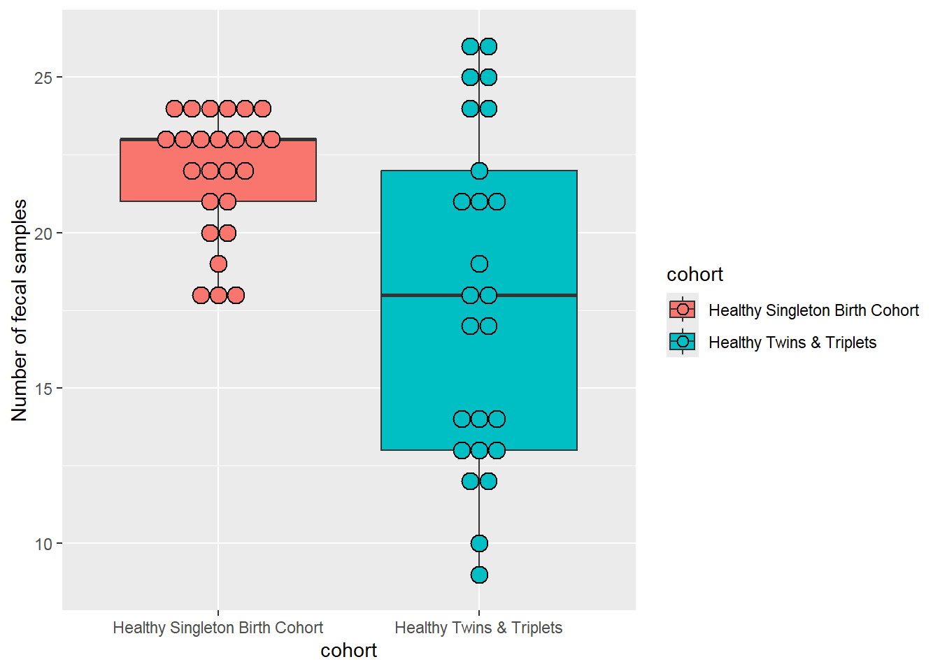

Violin Plot: similar to box plot but shows the density within groups, not much info provided as in box plot:

sh2 %>%
  group_by(cohort,child.id) %>%
  summarise(no.sam=n()) %>%
  ggplot(aes(x=cohort,y=no.sam,fill=cohort)) +
  geom_violin()+
  ylab("Number of fecal samples")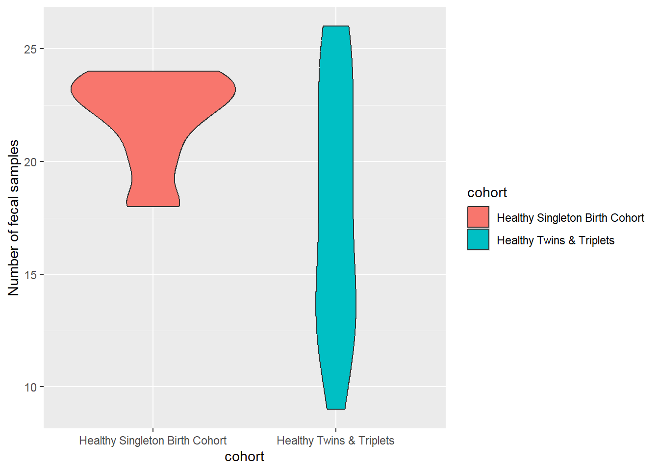

Bar plot number of fecal samples by cohort of singletons vs twins/triplets and summary of number of fecal samples:

nsam<-sh2 %>%
  group_by(cohort,child.id) %>%
  summarise(no.sam=n()) %>%
  #group_by(cohort) %>% 
  summarise(
    no.child = n(),
    mean = mean(no.sam, na.rm = TRUE),
    sd = sd(no.sam, na.rm = TRUE),
    se=sd/sqrt(n()),
    ci=1.96*se,
    median = median(no.sam, na.rm = TRUE),
    IQR = IQR(no.sam, na.rm = TRUE))
nsam

## # A tibble: 2 × 8
##   cohort                         no.child  mean    sd    se    ci median   IQR
##   <chr>                             <int> <dbl> <dbl> <dbl> <dbl>  <int> <dbl>
## 1 Healthy Singleton Birth Cohort       25  21.9  2.02 0.404 0.791     23     2
## 2 Healthy Twins & Triplets             25  17.9  5.34 1.07  2.09      18     9

Bar plot with error bar:

ggplot(nsam, aes(x=cohort, y=mean, fill=cohort)) + 
    geom_bar(position=position_dodge(), stat="identity") +
    geom_errorbar(aes(ymin=mean-se, ymax=mean+se),
                  width=.2,                    # Width of the error bars
                  position=position_dodge(.9))+
    ylab("Number of fecal samples (mean,se)")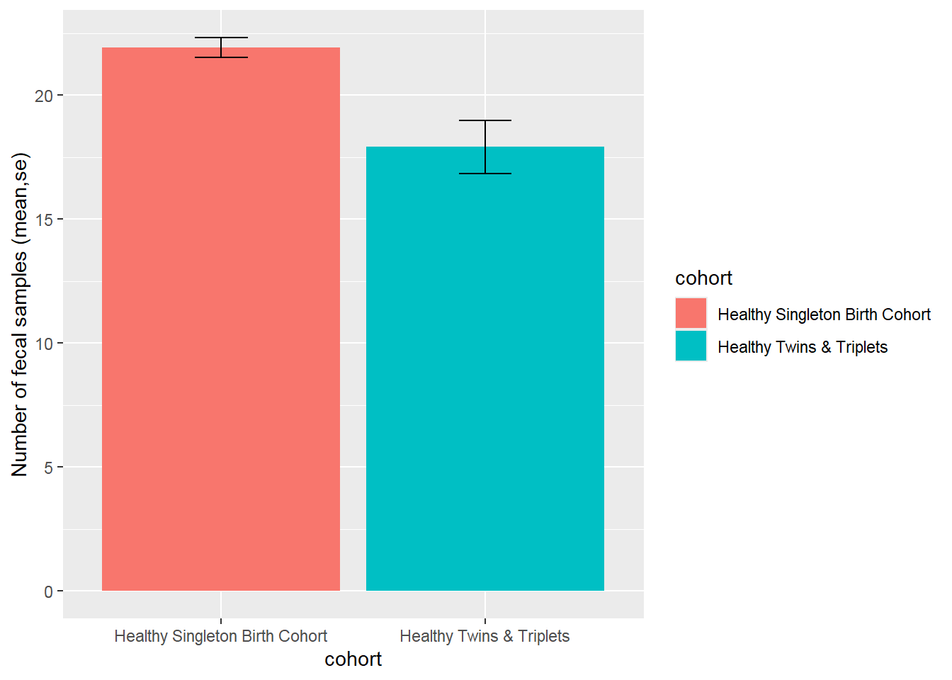

Bar plot with 95%CI:

ggplot(nsam, aes(x=cohort, y=mean, fill=cohort)) + 
    geom_bar(position=position_dodge(), stat="identity") +
    geom_errorbar(aes(ymin=mean-ci, ymax=mean+ci),
                  width=.2,                    # Width of the error bars
                  position=position_dodge(.9))+
    ylab("Number of fecal samples (mean, 95%CI)")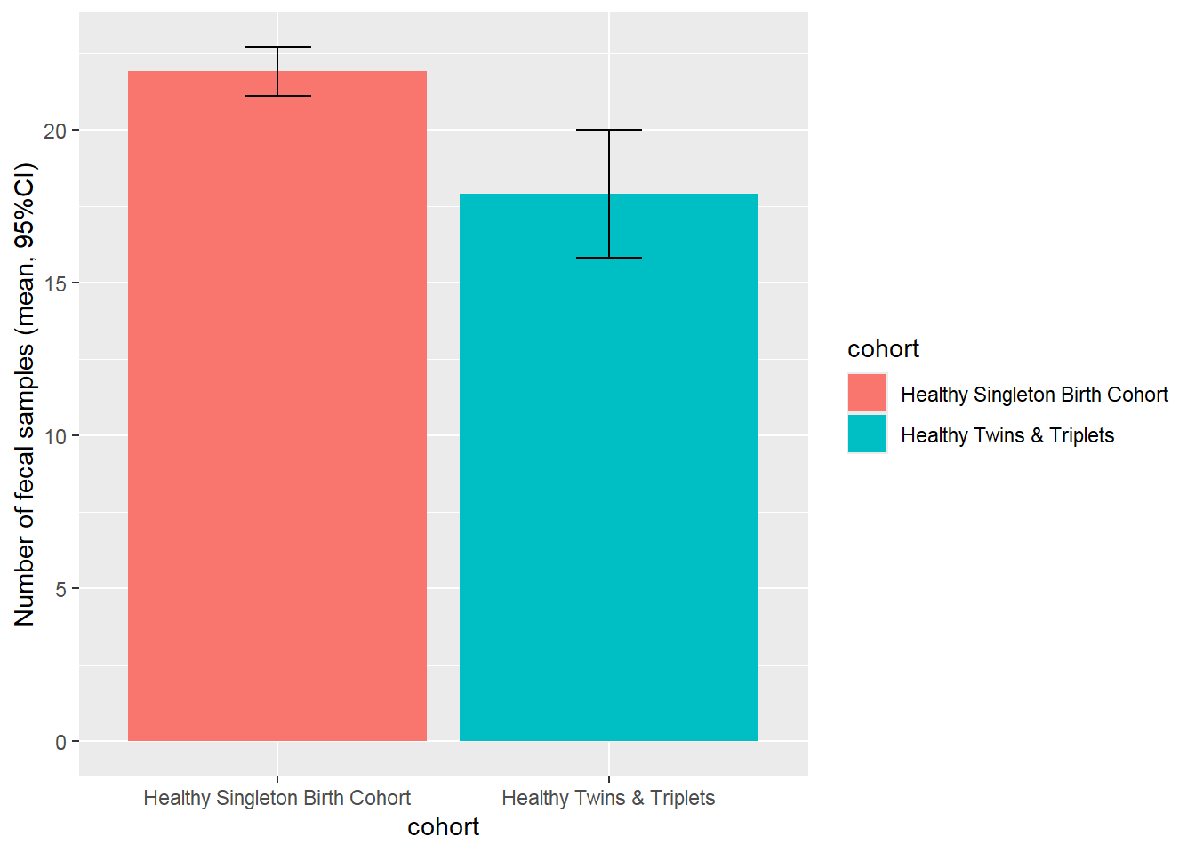

Histogram number of fecal samples by cohort of singletons vs twins/triplets:

sh2 %>%
  group_by(cohort,child.id) %>%
  summarise(no.sam=n()) %>%
  ggplot(aes(no.sam,y=..density..,fill=cohort))+
  geom_histogram(bins=10,alpha=0.5, position="identity")+
  geom_density(aes(no.sam,color=cohort),alpha=0.5)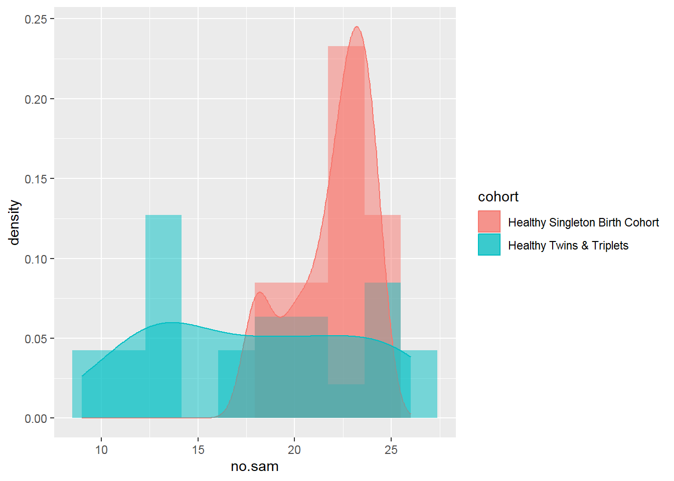

2.11.2 Further exploration

Basic statistical test:

nsam<-sh2 %>%
  group_by(cohort,child.id) %>%
  summarise(no.sam=n()) 
head(nsam)

## # A tibble: 6 × 3
## # Groups:   cohort [1]
##   cohort                         child.id  no.sam
##   <chr>                          <chr>      <int>
## 1 Healthy Singleton Birth Cohort Bgsng7018     21
## 2 Healthy Singleton Birth Cohort Bgsng7035     23
## 3 Healthy Singleton Birth Cohort Bgsng7052     20
## 4 Healthy Singleton Birth Cohort Bgsng7063     20
## 5 Healthy Singleton Birth Cohort Bgsng7071     18
## 6 Healthy Singleton Birth Cohort Bgsng7082     18

wilcox.test(no.sam~cohort,nsam)

## 
##  Wilcoxon rank sum test with continuity correction
## 
## data:  no.sam by cohort
## W = 443.5, p-value = 0.01092
## alternative hypothesis: true location shift is not equal to 0

kruskal.test(no.sam~cohort,nsam)

## 
##  Kruskal-Wallis rank sum test
## 
## data:  no.sam by cohort
## Kruskal-Wallis chi-squared = 6.5277, df = 1, p-value = 0.01062

t.test(no.sam~cohort,nsam)

## 
##  Welch Two Sample t-test
## 
## data:  no.sam by cohort
## t = 3.5045, df = 30.73, p-value = 0.001427
## alternative hypothesis: true difference in means between group Healthy Singleton Birth Cohort and group Healthy Twins & Triplets is not equal to 0
## 95 percent confidence interval:
##  1.671264 6.328736
## sample estimates:
## mean in group Healthy Singleton Birth Cohort       mean in group Healthy Twins & Triplets 
##                                        21.92                                        17.92

Which test is appropriate? => Please see Chapter “Basic Statistics” of this book.

Statistical test for difference in data type between sheet 1 and sheet 2?

Sheet 1 is cross sectional data.
Sheet 2 is longitudinal data: many observations per childid. Therefore, different ways of data description and analysis may be used.

Longitudinal data visualization with spaghetti plot:

sh2 %>%
  filter(!is.na(whz)) %>%
  ggplot()+ 
  geom_point(aes(x = age.m, y = whz, group = child.id, colour=cohort))+
  geom_line(aes(x = age.m, y = whz, group = child.id, colour=cohort),size=0.3)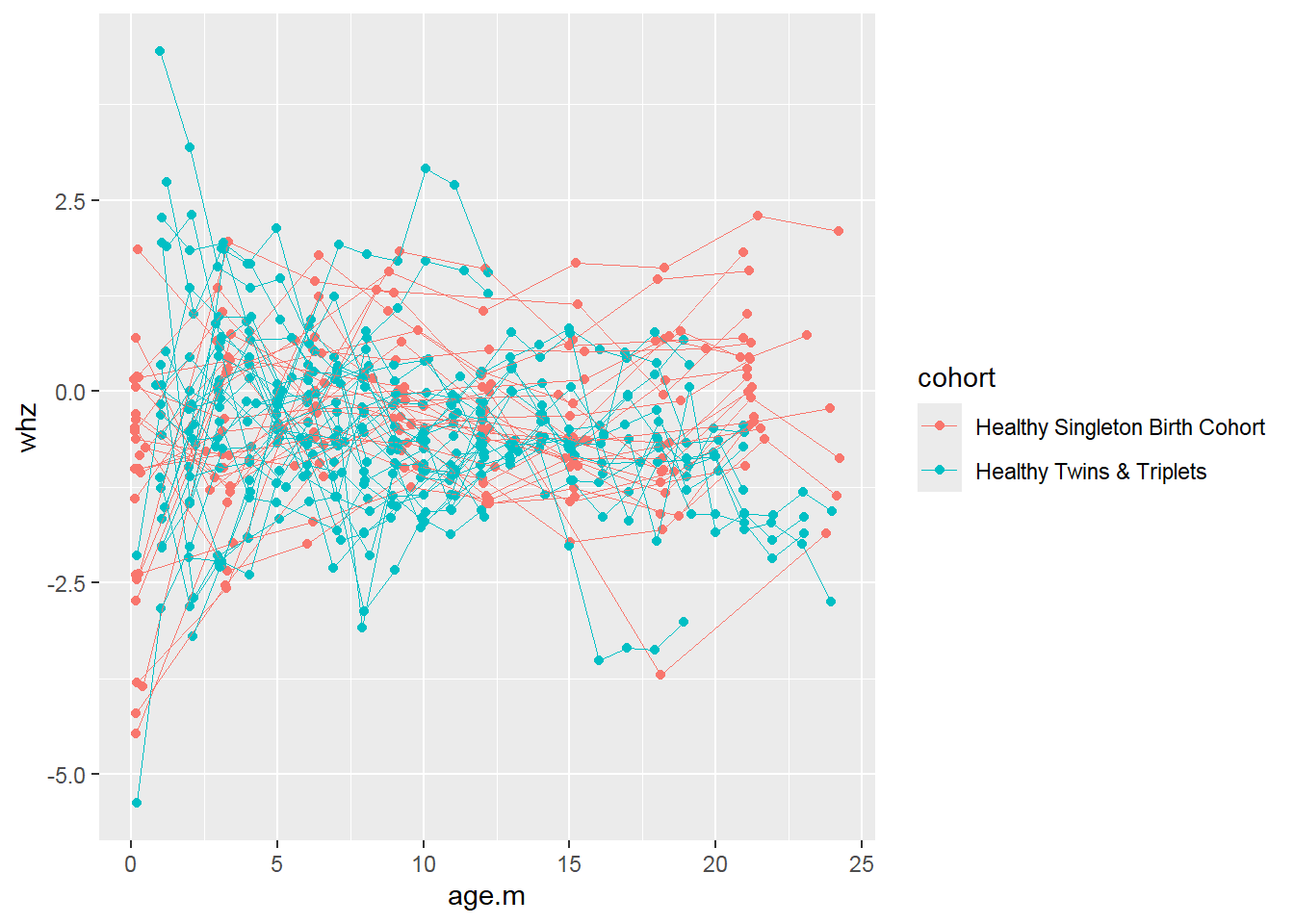

More exploration with waz:

sh2 %>%
  filter(!is.na(waz)) %>%
  ggplot()+
  geom_point(aes(x = age.m, y = waz, group = child.id, colour=cohort))+
  geom_line(aes(x = age.m, y = waz, group = child.id, colour=cohort),size=0.3)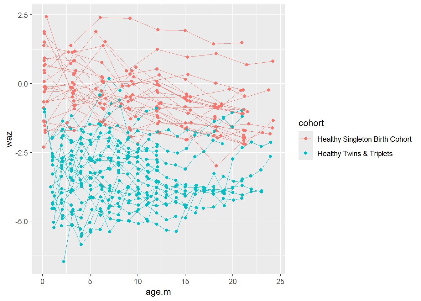

We can add fitted lines to the plot:

sh2 %>%
  filter(!is.na(waz)) %>%
  ggplot()+
  geom_point(aes(x = age.m, y = waz, group = child.id, colour=cohort))+
  geom_line(aes(x = age.m, y = waz, group = child.id, colour=cohort),size=0.3)+
  stat_smooth(aes(x = age.m, y = waz, colour=cohort), method = 'glm',size=2)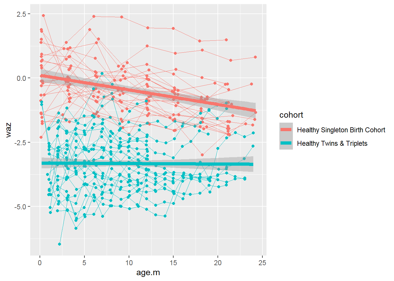

More exploration with haz:

sh2 %>%
  filter(!is.na(haz)) %>%
  ggplot()+
  geom_point(aes(x = age.m, y = haz, group = child.id, colour=cohort))+
  geom_line(aes(x = age.m, y = haz, group = child.id, colour=cohort),size=0.3)+
  stat_smooth(aes(x = age.m, y = haz, colour=cohort), method = 'glm',size=2)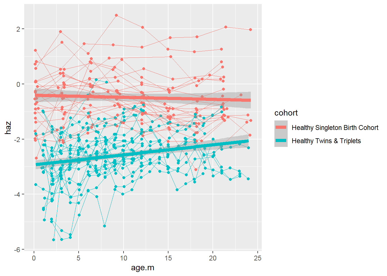

To test for the difference between two groups, check out the chapter “Longitudinal data analysis with R” in this book.

All-in-one spaghetti plot of three indices by cohort:

sh2 %>%
  filter(!is.na(haz) & !is.na(waz) & !is.na(whz)) %>%
  ggplot()+
  #add each item to the plot
  geom_point(aes(x = age.m, y = haz, group = child.id,color="haz"))+
  geom_line(aes(x = age.m, y = haz, group = child.id,color="haz"),size=0.3)+
  stat_smooth(aes(x = age.m, y = haz,color="haz"), method = 'glm',size=2)+
  geom_point(aes(x = age.m, y = waz, group = child.id,color="waz"))+
  geom_line(aes(x = age.m, y = waz, group = child.id,color="waz"),size=0.3)+
  stat_smooth(aes(x = age.m, y = waz,color="waz"), method = 'glm',size=2)+
  geom_point(aes(x = age.m, y = whz, group = child.id,color="whz"))+
  geom_line(aes(x = age.m, y = whz, group = child.id,color="whz"),size=0.3)+
  stat_smooth(aes(x = age.m, y = whz,color="whz"), method = 'glm',size=2)+
  #divide the plot into multiple panels (cohort groups)  
  facet_grid(.~ cohort)+
  theme(legend.title = element_blank())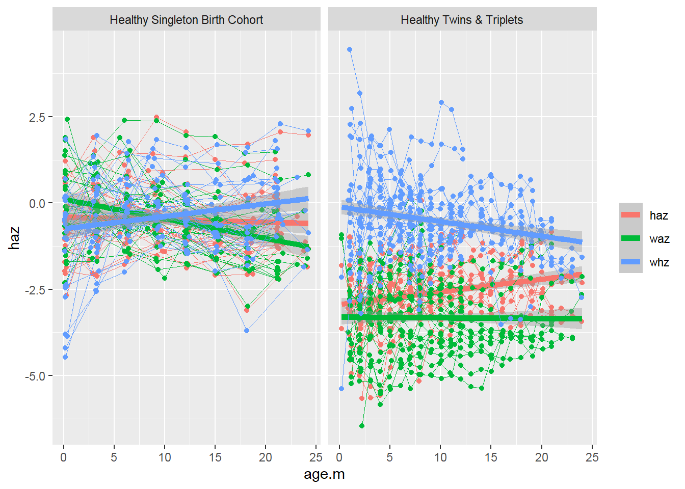

All-in-one spaghetti plot by cohort for each index and each plot for each index:

p1<-sh2 %>%
  filter(!is.na(haz) & !is.na(waz) & !is.na(whz)) %>%
  ggplot()+
  geom_point(aes(x = age.m, y = haz, group = child.id, colour=cohort))+
  geom_line(aes(x = age.m, y = haz, group = child.id, colour=cohort),size=0.3)+
  stat_smooth(aes(x = age.m, y = haz, colour=cohort), method = 'glm',size=2)+
  theme(legend.position = "bottom")
p2<-sh2 %>%
  filter(!is.na(haz) & !is.na(waz) & !is.na(whz)) %>%
  ggplot()+
  geom_point(aes(x = age.m, y = waz, group = child.id, colour=cohort))+
  geom_line(aes(x = age.m, y = waz, group = child.id, colour=cohort),size=0.3)+
  stat_smooth(aes(x = age.m, y = waz, colour=cohort), method = 'glm',size=2)+
  theme(legend.position = "bottom")
p3<-sh2 %>%
  filter(!is.na(haz) & !is.na(waz) & !is.na(whz)) %>%
  ggplot()+
  geom_point(aes(x = age.m, y = whz, group = child.id, colour=cohort))+
  geom_line(aes(x = age.m, y = whz, group = child.id, colour=cohort),size=0.3)+
  stat_smooth(aes(x = age.m, y = whz, colour=cohort), method = 'glm',size=2)+
  theme(legend.position = "bottom")
# Combine 3 plots into 1 plot
#install.packages("ggpubr")
library(ggpubr)
ggarrange(p1, p2, p3,nrow=1, common.legend = TRUE, legend="bottom")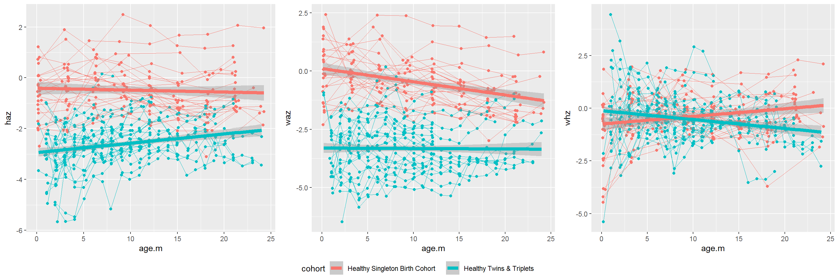

2.12 Reference materials

2.12.1 R books

2.12.2 Datasets

The datasets used in some examples of this book are of Bangladeshi infants published by Subramanian et al, Nature 2014. These datasets may be downloaded from Gordon’s lab website, or from my github repo.

References

Allaire, JJ, Yihui Xie, Christophe Dervieux, Jonathan McPherson, Javier Luraschi, Kevin Ushey, Aron Atkins, et al. 2024. Rmarkdown: Dynamic Documents for r. https://github.com/rstudio/rmarkdown.

Aragón, Tomás J. 2019. Population Health Data Science with r. 1st ed. Vol. 1. https://bookdown.org/taragonmd/phds/.

Chan, Chung-hong, Thomas J. Leeper, Jason Becker, and David Schoch. 2023. Rio: A Swiss-Army Knife for Data File i/o. https://cran.r-project.org/package=rio.

Heinzen, Ethan, Jason Sinnwell, Elizabeth Atkinson, Tina Gunderson, and Gregory Dougherty. 2021. Arsenal: An Arsenal of r Functions for Large-Scale Statistical Summaries. https://github.com/mayoverse/arsenal.

Ho, Nhan. 2020. metamicrobiomeR: Microbiome Data Analysis & Meta-Analysis with GAMLSS-BEZI & Random Effects. https://github.com/nhanhocu/metamicrobiomeR.

———. 2024b. R: A Language and Environment for Statistical Computing. Vienna, Austria: R Foundation for Statistical Computing. https://www.R-project.org/.

Subramanian, Sathish, Sayeeda Huq, Tanya Yatsunenko, Rashidul Haque, Mustafa Mahfuz, Mohammed A. Alam, Amber Benezra, et al. 2014. “Persistent Gut Microbiota Immaturity in Malnourished Bangladeshi Children.” Nature 510: 417–21. https://doi.org/10.1038/nature13421.

———. 2023b. Tidyverse: Easily Install and Load the Tidyverse. https://tidyverse.tidyverse.org.