Chapter 6 Linear regression with R

Nhan Thi Ho, MD, PhD

6.1 Introduction to linear regression

Linear regression evaluates the relationship between a dependent variable (outcome) and one or more independent variables (predictors). From a sample data, linear regression is used to estimate population parameters characterizing these relationships and their uncertainties. Linear regression helps us estimate the effect of a predictor while controlling for other variables and helps predict outcomes for future observations.

6.2 Simple linear regression

6.2.1 Simple linear model with R

Simple linear regression quantifies the relationship between one outcome and one predictor. Below is an generated example data:

##          x         y
## 1 3.620757 0.8449674
## 2 3.035641 0.8304951
## 3 3.773154 0.9622945
## 4 4.272489 0.9096735
## 5 3.370975 0.8072324
## 6 2.837146 0.8259437

In which:

y is outcome or response or dependent variable (DV)
x is predictor or regressor or independent variable (IV)

Simple linear regression assumes the linear relationship between x and y. The formula for simple linear regression model may be written as: $y = \beta_0 + \beta_1 x + \epsilon$ In which:

$\beta_0$ is the intercept or the predicted $y$ when $x=0$
$\beta_1$ is the slope or the predicted change in $y$ for a one-unit increase in $x$
$\epsilon$ is the error term or the deviation of the predicted $y$ value from the observed $y$ .

Simple linear model may be fitted in R as below (R Core Team 2024b):

slm.fit <- lm(y ~ x, data = df)

The lm() returns complex objects which may be examined by:

coef(): model coefficients
summary(): coefficients, standard errors, p-values, model F-test, etc.
predict(): model predictions
residuals(): various kinds of residuals
confint(): confidence intervals for coefficients
plot(): diagnostic plots

The result output may be summarized as below:

summary(slm.fit)

## 
## Call:
## lm(formula = y ~ x, data = df)
## 
## Residuals:
##      Min       1Q   Median       3Q      Max 
## -0.25771 -0.07126  0.00101  0.05635  0.32485 
## 
## Coefficients:
##             Estimate Std. Error t value Pr(>|t|)    
## (Intercept) 0.525215   0.019149   27.43   <2e-16 ***
## x           0.111954   0.006056   18.48   <2e-16 ***
## ---
## Signif. codes:  0 '***' 0.001 '**' 0.01 '*' 0.05 '.' 0.1 ' ' 1
## 
## Residual standard error: 0.1034 on 298 degrees of freedom
## Multiple R-squared:  0.5342, Adjusted R-squared:  0.5326 
## F-statistic: 341.7 on 1 and 298 DF,  p-value: < 2.2e-16

The summary() outputs show:

Model formula
Summary of residual distribution
Estimated coefficients, standard errors, t-values, and p-values (for testing a hypothesis that a coefficient equals to zero).
A quick visual shortcut to p-values by *
Residual standard error measuring the average amount that observed responses deviate from the fitted regression line.
Degrees of freedom ( $df$ ) represent the number of independent observations ( $N$ ) in the data that are available to estimate a parameter. For linear regression, $p =$ the number of predictors $+ 1$ and $df = N - p$ .
R-square ( $R^2$ ), a measure to test if the model is a good fit, shows the amount of variance of y explained by x. $R^2 = Explained \ variation \ of \ the \ model \ / \ Total \ variation \ of \ the \ model$ . If the model fit the data well, $R^2$ is near 1 and if the model fit the data poorly, $R^2$ is near 0. $Adjusted \ R^2$ shows the same as $R^2$ but adjusted by the number of cases and number of variables. When the number of variables is small and the number of outcomes is very large then $Adjusted \ R^2$ is closer to $R^2$ .
$F$ -statistic: indicates whether the overall model is statistically significant (at least one predictor is related to the outcome)

The summary output above show that x is positively and significantly associated with y. One unit increase in x is associated with 0.1119536 increase of y.

Confidence intervals may be computed with confint():

ci <- confint(slm.fit)
ci

##                 2.5 %    97.5 %
## (Intercept) 0.4875300 0.5628993
## x           0.1000348 0.1238724

The intercept, the slope and residuals are visualized as below:

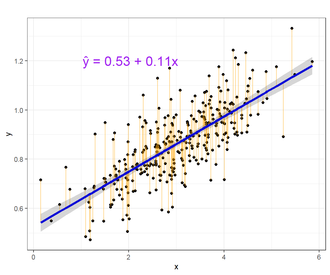
The straight blue line in the image above represents the predicted values. The model fit may be assessed by plotting the predicted values to evaluate if they look reasonable against the observed data.The shaded area represent the confidence interval of predicted values.

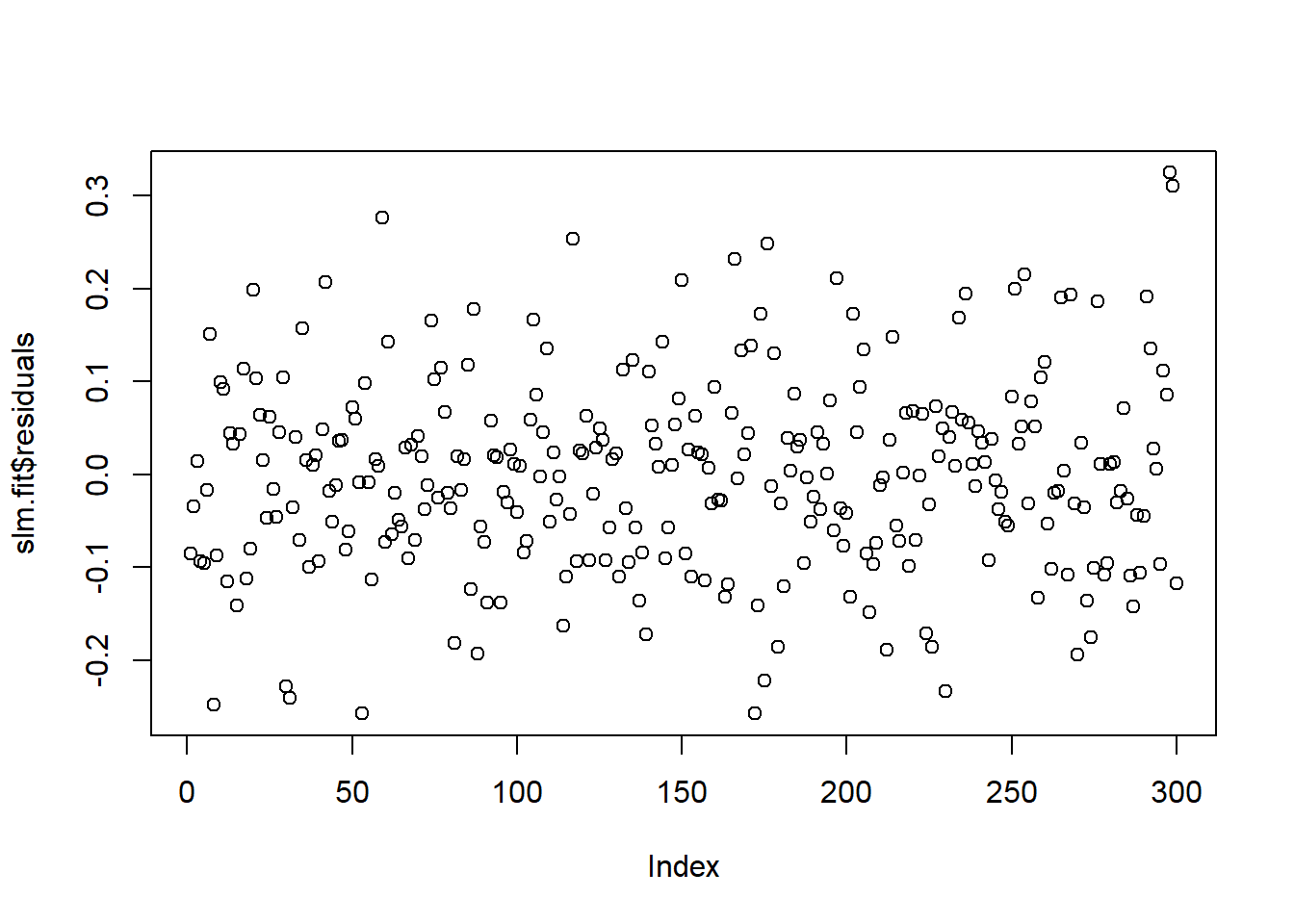
The orange vertical line from the straight line to the observed data value is the residual. For a good model, the sum of the residuals should be approximately zero or as low as possible and the residual plot should look random. If there is pattern in the residual plot, the simple linear model may not fit the data well and there may be a need to transform the variable (e.g. adding quadratic, or cubic term,…). The residuals may plotted in R as below:

plot(slm.fit$residuals)

6.2.2 Linear model assumptions

Below are assumptions for inferences made from a regression model.

L: Linear relationship between the mean outcome (Y) and the predictor variable (X)
I: The errors are independent
N: The outcomes are normally distributed at each level of predictor variable (X)
E: The variance of the outcomes is equal for all levels of predictor variable (X)

If the assumptions are violated, the model estimates and inferences may not be valid.

6.2.3 Checking linear model assumptions

6.2.3.1 Linear assumption

If linear assumption is met, the residuals should be random and there should be no systematic trend or pattern in residual plot.

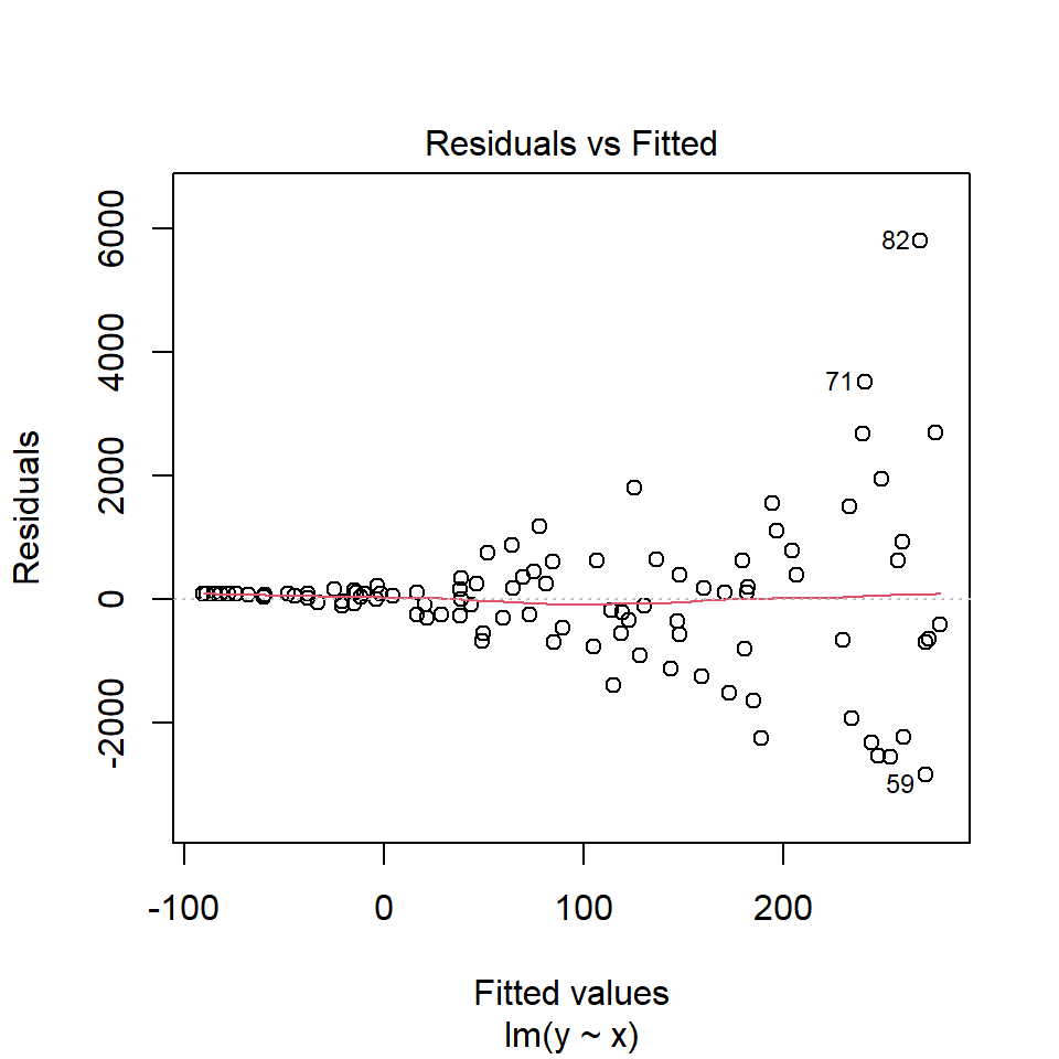
Diagnostic plots may be done by plot() on the lm object. The first plot is the residuals vs fitted values plot.

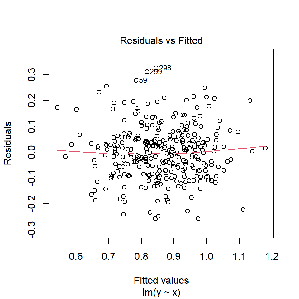
# which = 1 plots residuals vs.fitted values plot 
plot(slm.fit, which=1)

In our example, there is no trend in residual plot.

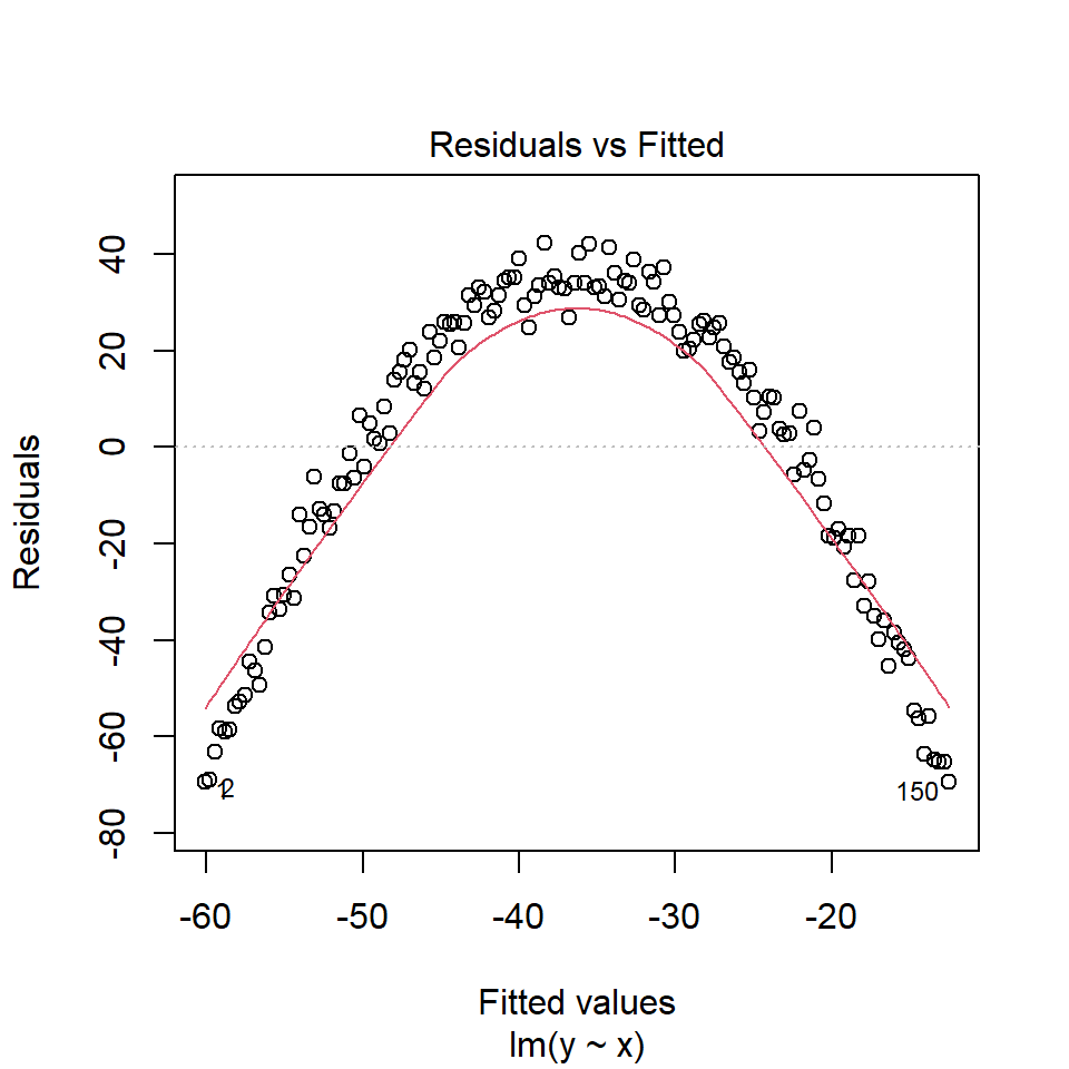
If there is a trend in the residuals, it suggests a nonlinear relationship between predictor and outcome variables. In this case, one may consider adding non-linear term to the model (e.g. cubic, quadratic, splines,…) or using non-linear transformations (e.g. logarithm) to either predictor or outcome variables.

Below is an example plot showing a clear trend of residuals:

6.2.3.2 Equal variance assumption (Homoscedasticity)

If this assumption is violated, standard errors will be inaccurate resulting in inaccurate test statistics, confidence intervals and p-values. For this assumption, the diagnostic plot of residuals vs. fitted values should show random scatter around the zero line with equal spread across the range of fitted values as in the residual plot of our example.

# which = 1 plots residuals vs.fitted values plot 
plot(slm.fit, which=1)

Unequal variance or heteroscedasticity is often observed in the form of increasing variance of the residuals with increasing fitted values:

If equal variance assumption is violated, one may consider:

Transformation of variables (e.g., log transformation of the outcome variable)
Using robust standard errors (heteroscedastic-consistent or “sandwich”) (may be done with R package “sandwich”)
Using a mixed model for heteroscedasticity modeling (may be done with R package “nlme”)

6.2.3.3 Independence assumption

If this assumption is violated, it may affect the accuracy of confidence intervals and p-values.

Common causes of data dependency are:

Sampling in clusters
Repeated measurements of the same subjects

The approaches to handle this assumption violation are:

Model data dependency with mixed/multilevel models, fixed effect models, … (may be done with R package “lme4” )
Using cluster robust standard errors

6.2.3.4 Normal distribution assumption

If the errors are not normally distributed, the accuracy of confidence interval and p-values may be affected, especially in case of small sample size (the impact is less with large sample size).

Histogram and q-q plot of residuals may be used as diagnostic plots:

# A simple histogram of residuals
hist(slm.fit$residuals, breaks=20)

# Normal Quantile to Quantile plot
qqnorm(slm.fit$residuals)
qqline(slm.fit$residuals)

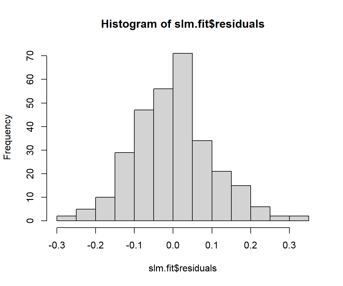
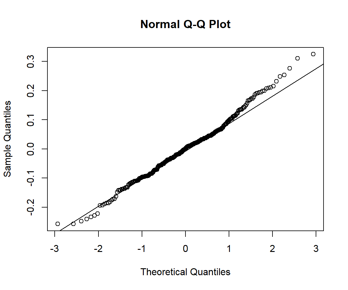
If the errors are not normally distributed, the q-q plot will show deviation from the diagonal line. The approaches to handle this issue may be:

Transformation (e.g. logarithm,…) of the outcome variable
Using using generalized linear model (may be done with glm() function)

6.2.4 Checking influential observations

Influential observations change model estimates substantially when included vs when excluded from the data. Model coefficients change when a particular observation is excluded may be evaluated by influence diagnostic measures:

dfbeta measures how a specific coefficient changes when deleting an observation
Cook’s distance measures how much all coefficients change when deleting an observation

Influence diagnostic measures may be done with influence.measures() on an lm object, which results in several influence measures including dfbetas for each coefficient and Cook’s distance.

If there are any unusually large influence measures, it will be flagged by an * in the infl column.

influence <- influence.measures(slm.fit)
#influence

6.2.5 Categorical predictor variables

Categorical variables with k (>=2) categories will have k-1 coefficient estimates. The simplest categorical variable is dummy variable with 2 categories 0 and 1 denoting not belonging or belonging to a category. An example of this dummy variable may be smoker with category “no” (equivalent to 1) and “yes” (equivalent to 1). Categorical variables with k categories is treated as k-1 dummy variables with the omitted category treated as reference category. Categorical variables in R are represented by factor variables and the factor order and reference group may be selected. When performing lm(), R will automatically create dummy variables for each level of factor except for the first level (which is used as the reference group).

6.2.5.1 Example simple linear regression with categorical predictor variable

We will use example data regarding the association of medical costs and patient information. We first load the data and summarize all variables with the “arsenal” package (Heinzen et al. 2021).

# Load example linear regression data 
dlm<-read.csv("https://raw.githubusercontent.com/stedy/Machine-Learning-with-R-datasets/master/insurance.csv")
colnames(dlm)<-tolower(colnames(dlm))
str(dlm)

## 'data.frame':    1338 obs. of  7 variables:
##  $ age     : int  19 18 28 33 32 31 46 37 37 60 ...
##  $ sex     : chr  "female" "male" "male" "male" ...
##  $ bmi     : num  27.9 33.8 33 22.7 28.9 ...
##  $ children: int  0 1 3 0 0 0 1 3 2 0 ...
##  $ smoker  : chr  "yes" "no" "no" "no" ...
##  $ region  : chr  "southwest" "southeast" "southeast" "northwest" ...
##  $ charges : num  16885 1726 4449 21984 3867 ...

#turn character variables into factor variables
dlm[,colnames(dplyr::select_if(dlm, is.character))] <- lapply(dlm[,colnames(dplyr::select_if(dlm, is.character))], as.factor)

#summary of all variables in the dataset
my_controls <- tableby.control(
  numeric.stats = c("meansd", "medianq1q3","meanCI","range","Nmiss2"),
  cat.stats = c("countpct", "Nmiss2"),
  stats.labels = list(
    meansd = "Mean (SD)",
    medianq1q3 = "Median (Q1, Q3)",
    range = "Min - Max",
    Nmiss2 = "Missing",
    meanCI = "Mean (95%CI)"
  )
)
mylabels <-as.list(colnames(dlm))
names(mylabels)<-colnames(dlm)
tabs <- tableby(as.formula(paste("",paste(colnames(dlm),collapse="+"),sep="~")),
                data = dlm,
                control = my_controls) 
kable(summary(tabs,labelTranslations = mylabels, text=TRUE))

	Overall (N=1338)
age
- Mean (SD)	39.207 (14.050)
- Median (Q1, Q3)	39.000 (27.000, 51.000)
- Mean (95%CI)	39.207 (38.454, 39.961)
- Min - Max	18.000 - 64.000
- Missing	0
sex
- female	662 (49.5%)
- male	676 (50.5%)
- Missing	0
bmi
- Mean (SD)	30.663 (6.098)
- Median (Q1, Q3)	30.400 (26.296, 34.694)
- Mean (95%CI)	30.663 (30.336, 30.990)
- Min - Max	15.960 - 53.130
- Missing	0
children
- Mean (SD)	1.095 (1.205)
- Median (Q1, Q3)	1.000 (0.000, 2.000)
- Mean (95%CI)	1.095 (1.030, 1.160)
- Min - Max	0.000 - 5.000
- Missing	0
smoker
- no	1064 (79.5%)
- yes	274 (20.5%)
- Missing	0
region
- northeast	324 (24.2%)
- northwest	325 (24.3%)
- southeast	364 (27.2%)
- southwest	325 (24.3%)
- Missing	0
charges
- Mean (SD)	13270.422 (12110.011)
- Median (Q1, Q3)	9382.033 (4740.287, 16639.913)
- Mean (95%CI)	13270.422 (12620.954, 13919.890)
- Min - Max	1121.874 - 63770.428
- Missing	0

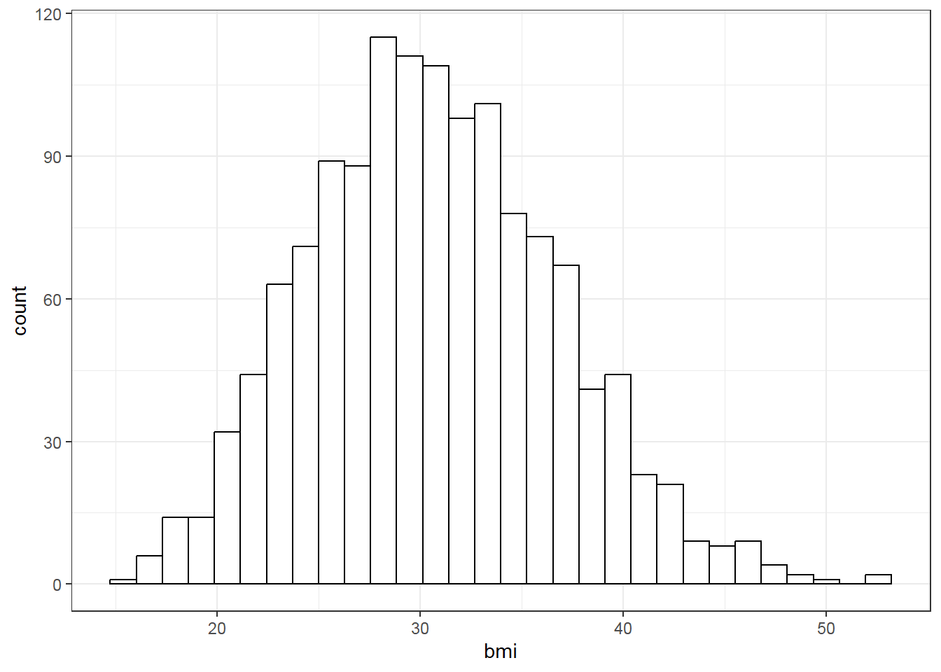
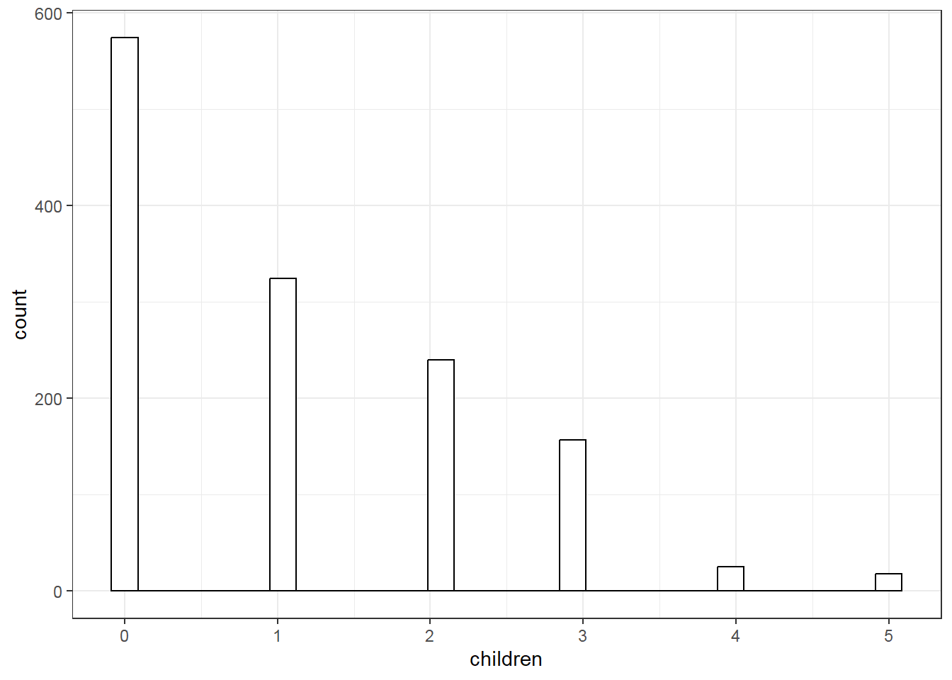
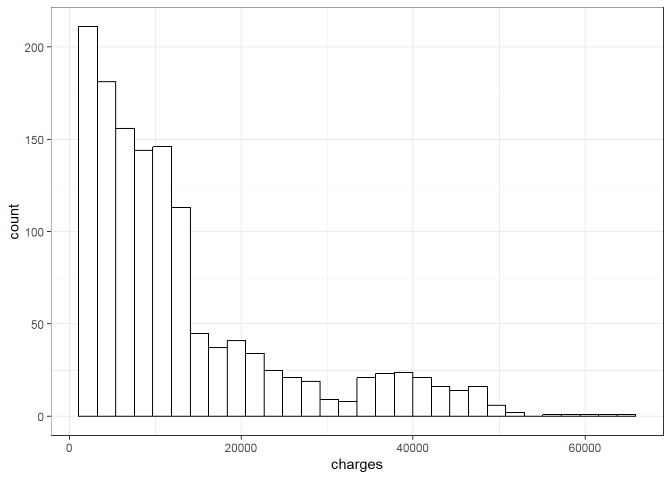
We then examine data distribution with histogram:

# Data distribution plot
vars<-colnames(dplyr::select_if(dlm, is.numeric))
for (i in 1:length(vars)){
    print(ggplot(data=dlm, aes(x=dlm[,vars[i]])) + 
            geom_histogram(colour="black", fill="white") +
            theme_bw()+
            labs(x=vars[i]))}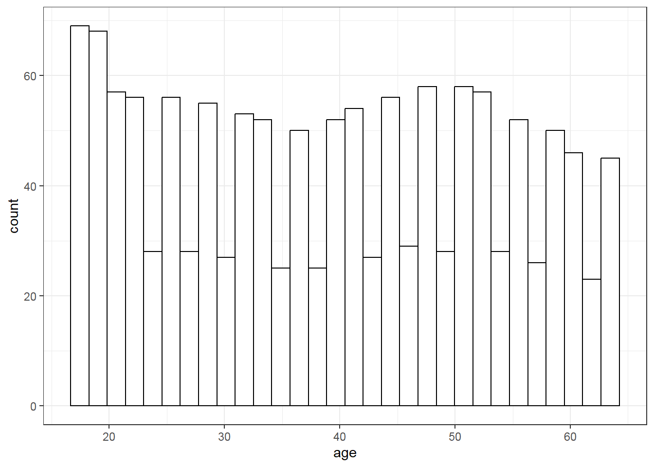

We fit an example simple linear model with charges as outcome and smoker as categorical predictor.

flm<-lm(charges ~ smoker, data=dlm)
sumflm<-summary(flm)
sumflm

## 
## Call:
## lm(formula = charges ~ smoker, data = dlm)
## 
## Residuals:
##    Min     1Q Median     3Q    Max 
## -19221  -5042   -919   3705  31720 
## 
## Coefficients:
##             Estimate Std. Error t value Pr(>|t|)    
## (Intercept)   8434.3      229.0   36.83   <2e-16 ***
## smokeryes    23616.0      506.1   46.66   <2e-16 ***
## ---
## Signif. codes:  0 '***' 0.001 '**' 0.01 '*' 0.05 '.' 0.1 ' ' 1
## 
## Residual standard error: 7470 on 1336 degrees of freedom
## Multiple R-squared:  0.6198, Adjusted R-squared:  0.6195 
## F-statistic:  2178 on 1 and 1336 DF,  p-value: < 2.2e-16

# Add confidence interval to summary
ciflm <- confint(flm)
sumciflm <- cbind(sumflm$coefficients, ciflm)
round(sumciflm, 4)

##              Estimate Std. Error t value Pr(>|t|)     2.5 %    97.5 %
## (Intercept)  8434.268   229.0142 36.8286        0  7985.002  8883.535
## smokeryes   23615.964   506.0753 46.6649        0 22623.175 24608.752

From the output, smoker= no is expected to have charges of 8434.2682979 and smoker = yes is expected to have charges of 2.3615964^{4} higher than smoker= no.

Predicted charges for smokers and non-smokers may be calculated and visualized as below.

predictions <- predict(flm, newdata=dlm, interval="confidence")
new_data <- cbind(dlm, as.data.frame(predictions))
#plot 
ggplot(dlm, aes(smoker, charges)) +
  geom_point(color="grey32",size=0.75) +
  geom_errorbar(data = new_data, aes(x=smoker, ymin=lwr, ymax=upr, color=smoker),
                width=0.1) +
  geom_point(data = new_data, aes(smoker, fit, color=smoker), size = 3) +
  labs(x = "smoker", y = "charges") +
  theme_bw()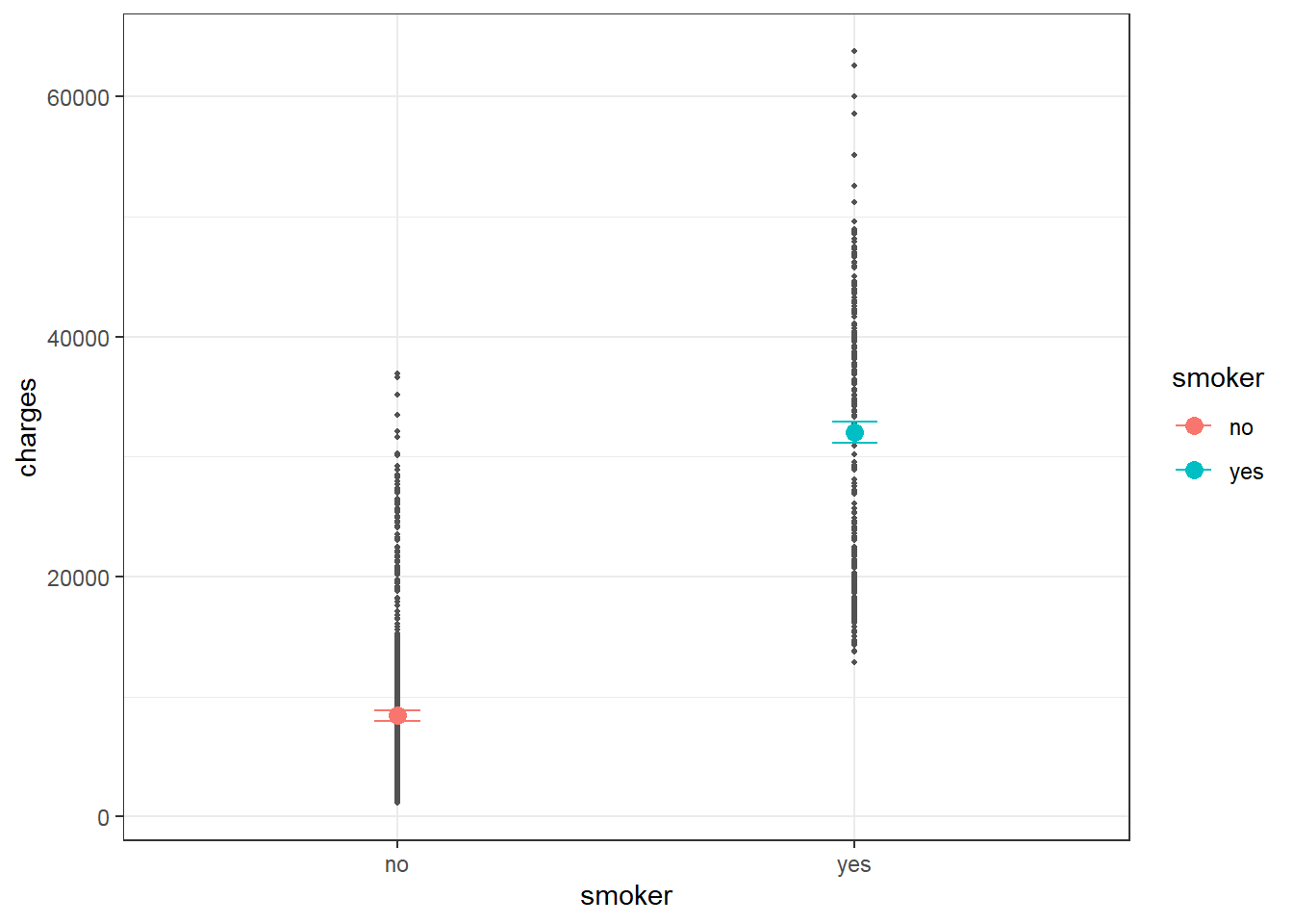

The plot shows clear difference in predicted charges between non-smoker and smoker corresponding to significant coefficient of smoker in the simple linear model.

We fit another example simple linear model with charges as outcome and region as categorical predictor (region has 4 categories).

flm.r<-lm(charges ~ region, data=dlm)
sumflm.r<-summary(flm.r)
sumflm.r

## 
## Call:
## lm(formula = charges ~ region, data = dlm)
## 
## Residuals:
##    Min     1Q Median     3Q    Max 
## -13614  -8463  -3793   3385  49035 
## 
## Coefficients:
##                 Estimate Std. Error t value Pr(>|t|)    
## (Intercept)      13406.4      671.3  19.971   <2e-16 ***
## regionnorthwest   -988.8      948.6  -1.042    0.297    
## regionsoutheast   1329.0      922.9   1.440    0.150    
## regionsouthwest  -1059.4      948.6  -1.117    0.264    
## ---
## Signif. codes:  0 '***' 0.001 '**' 0.01 '*' 0.05 '.' 0.1 ' ' 1
## 
## Residual standard error: 12080 on 1334 degrees of freedom
## Multiple R-squared:  0.006634,   Adjusted R-squared:  0.0044 
## F-statistic:  2.97 on 3 and 1334 DF,  p-value: 0.03089

# Add confidence interval to summary
ciflm.r <- confint(flm.r)
sumciflm.r <- cbind(sumflm.r$coefficients, ciflm.r )
round(sumciflm.r, 4)

##                   Estimate Std. Error t value Pr(>|t|)      2.5 %     97.5 %
## (Intercept)     13406.3845   671.2966 19.9709   0.0000 12089.4724 14723.2966
## regionnorthwest  -988.8091   948.6263 -1.0424   0.2974 -2849.7709   872.1526
## regionsoutheast  1329.0269   922.9071  1.4400   0.1501  -481.4805  3139.5343
## regionsouthwest -1059.4471   948.6263 -1.1168   0.2643 -2920.4089   801.5146

region = northest is used as reference group and other region categories are turned into 3 dummy variables and are compared with the reference group northest. From the output, region northest is predicted to have charges of 1.3406385^{4}. Region northwest is predicted to have charges of 988.8091424 lower than region northest. Region southeast is predicted to have charges of 1329.0269212 higher than region northest, and so on. However, the difference between region categories are not significant.

Predicted charges for region may be calculated and visualized as below.

predictions <- predict(flm.r, newdata=dlm, interval="confidence")
new_data <- cbind(dlm, as.data.frame(predictions))
#plot 
ggplot(new_data, aes(region, charges)) +
  geom_point(color="grey32",size=0.75) +
  geom_errorbar(data = new_data, aes(x=region, ymin=lwr, ymax=upr, color=region),
                width=0.1) +
  geom_point(data = new_data, aes(region, fit, color=region), size = 3) +
  labs(x = "region", y = "charges") +
  theme_bw()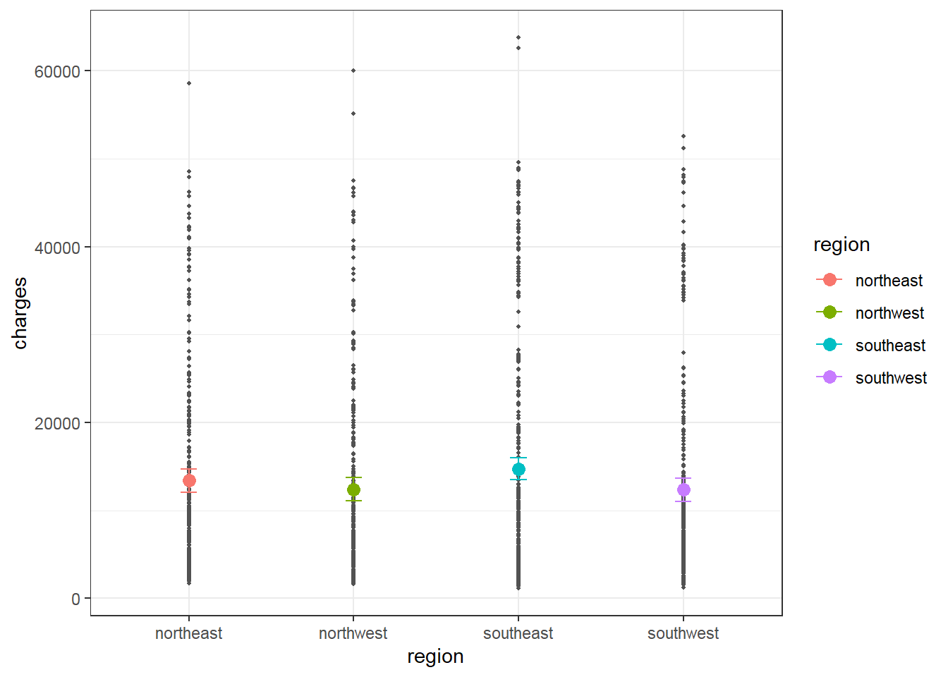

The plot shows similar predicted charges between region categories, which is corresponding to non-significant coefficients of region categories vs. reference category northeast.

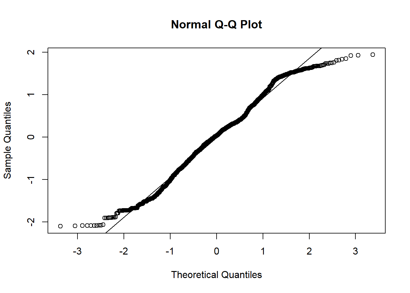
Diagnostic plots may be done with residual vs. fitted plot for homoscedasticity and q-q plot for normality of residuals:

plot(flm.r, which = 1)

qqnorm(residuals(flm.r))
qqline(residuals(flm.r))

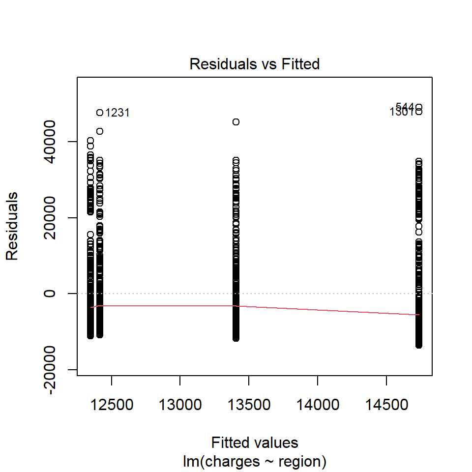
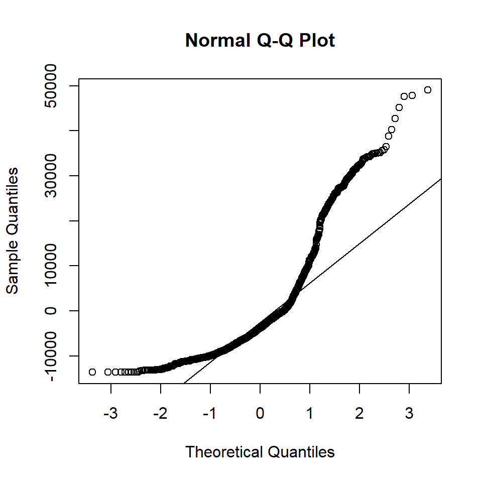
With the above plot, normality assumption seems not met. The histogram of charges also shows skewed distribution. Therefore, one may try logarithm transformation of the outcome charges, refit linear model and re-perform diagnostic plots.

dlm$logcharges<-log(dlm$charges)
flm.lr<-lm(logcharges ~ region, data=dlm)
sumflm.lr<-summary(flm.lr)
sumflm.lr

## 
## Call:
## lm(formula = logcharges ~ region, data = dlm)
## 
## Residuals:
##      Min       1Q   Median       3Q      Max 
## -2.09965 -0.64192  0.03622  0.62333  1.94064 
## 
## Coefficients:
##                 Estimate Std. Error t value Pr(>|t|)    
## (Intercept)      9.16877    0.05106 179.562   <2e-16 ***
## regionnorthwest -0.09903    0.07216  -1.372   0.1701    
## regionsoutheast -0.04637    0.07020  -0.660   0.5091    
## regionsouthwest -0.13767    0.07216  -1.908   0.0566 .  
## ---
## Signif. codes:  0 '***' 0.001 '**' 0.01 '*' 0.05 '.' 0.1 ' ' 1
## 
## Residual standard error: 0.9191 on 1334 degrees of freedom
## Multiple R-squared:  0.003143,   Adjusted R-squared:  0.0009012 
## F-statistic: 1.402 on 3 and 1334 DF,  p-value: 0.2406

# Add confidence interval to summary
ciflm.lr <- confint(flm.lr)
sumciflm.lr <- cbind(sumflm.lr$coefficients, ciflm.lr)
round(sumciflm.lr, 4)

##                 Estimate Std. Error  t value Pr(>|t|)   2.5 % 97.5 %
## (Intercept)       9.1688     0.0511 179.5621   0.0000  9.0686 9.2689
## regionnorthwest  -0.0990     0.0722  -1.3725   0.1701 -0.2406 0.0425
## regionsoutheast  -0.0464     0.0702  -0.6605   0.5091 -0.1841 0.0913
## regionsouthwest  -0.1377     0.0722  -1.9079   0.0566 -0.2792 0.0039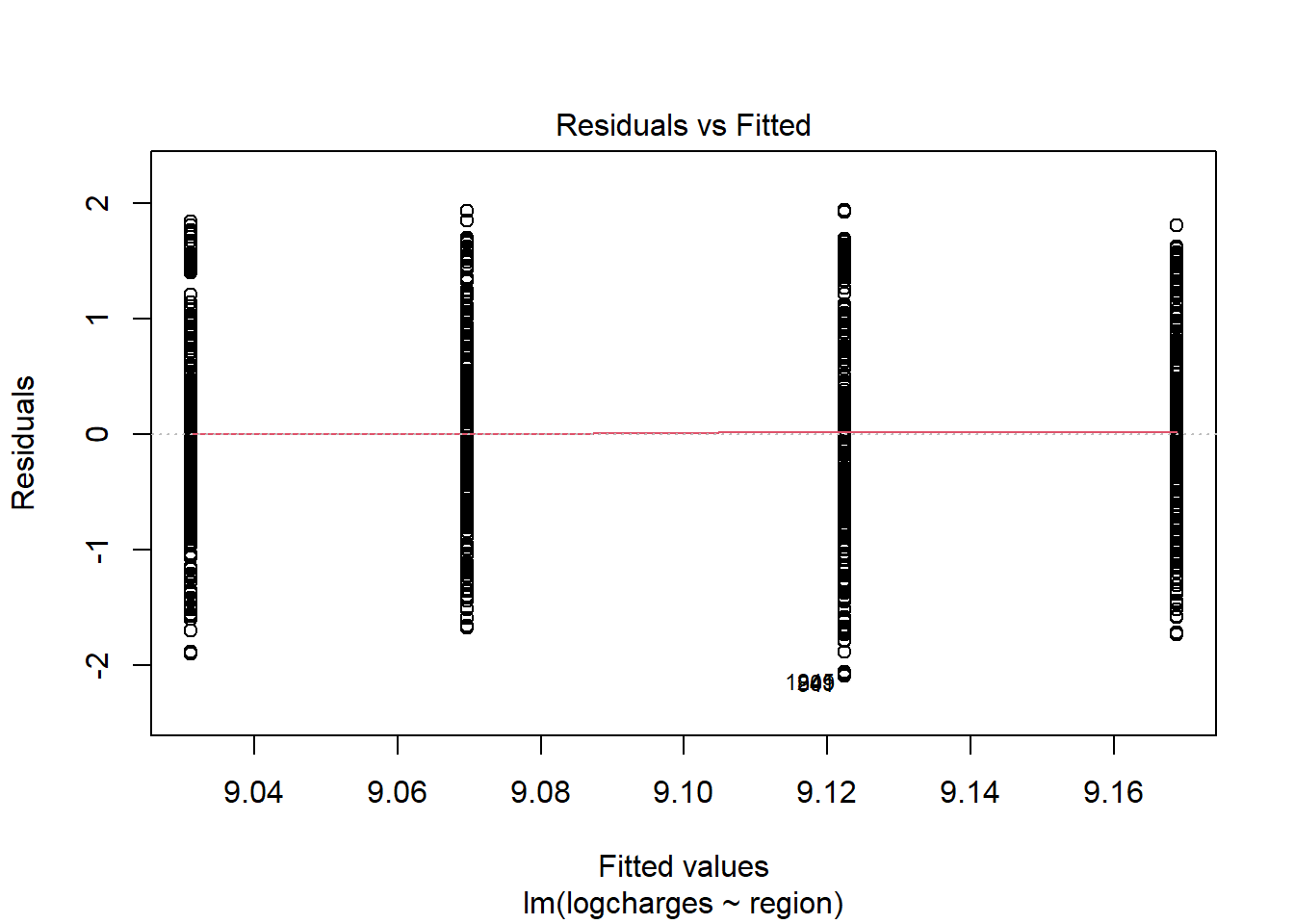

#diagnostic plot
plot(flm.lr, which = 1)

qqnorm(residuals(flm.lr))
qqline(residuals(flm.lr))

The diagnostic plots look better after logarithm transformation of the outcome charges.

6.3 Multiple linear regression

Multiple linear regression allows the estimation of the effects of multiple predictor variables simultaneously on outcome variable. For the example medical costs and patient information data above, multiple linear regression may be done by adding several variables as predictors in the linear model, for example bmi and smoker as predictors and logarithm of charges (logcharges) as outcome.

# Simple linear regression model with only bmi as predictor and logarithm charges as outcome 
flm.b<-lm(logcharges ~ bmi, data=dlm)
sumflm.b<-summary(flm.b)
sumflm.b

## 
## Call:
## lm(formula = logcharges ~ bmi, data = dlm)
## 
## Residuals:
##      Min       1Q   Median       3Q      Max 
## -2.48894 -0.63536  0.03136  0.68007  1.95182 
## 
## Coefficients:
##             Estimate Std. Error t value Pr(>|t|)    
## (Intercept) 8.485243   0.127833  66.378  < 2e-16 ***
## bmi         0.020005   0.004089   4.892 1.12e-06 ***
## ---
## Signif. codes:  0 '***' 0.001 '**' 0.01 '*' 0.05 '.' 0.1 ' ' 1
## 
## Residual standard error: 0.9117 on 1336 degrees of freedom
## Multiple R-squared:  0.0176, Adjusted R-squared:  0.01687 
## F-statistic: 23.94 on 1 and 1336 DF,  p-value: 1.117e-06

# Add confidence interval to summary
ciflm.b <- confint(flm.b)
sumciflm.b <- cbind(sumflm.b$coefficients, ciflm.b)
round(sumciflm.b, 4)

##             Estimate Std. Error t value Pr(>|t|)  2.5 % 97.5 %
## (Intercept)   8.4852     0.1278 66.3778        0 8.2345  8.736
## bmi           0.0200     0.0041  4.8925        0 0.0120  0.028

# Simple linear regression model with only smoker as predictor and logarithm charges as outcome 
flm.s<-lm(logcharges ~ smoker, data=dlm)
sumflm.s<-summary(flm.s)
sumflm.s

## 
## Call:
## lm(formula = logcharges ~ smoker, data = dlm)
## 
## Residuals:
##     Min      1Q  Median      3Q     Max 
## -1.7655 -0.4370  0.1237  0.4785  1.7280 
## 
## Coefficients:
##             Estimate Std. Error t value Pr(>|t|)    
## (Intercept)  8.78823    0.02105  417.52   <2e-16 ***
## smokeryes    1.51588    0.04651   32.59   <2e-16 ***
## ---
## Signif. codes:  0 '***' 0.001 '**' 0.01 '*' 0.05 '.' 0.1 ' ' 1
## 
## Residual standard error: 0.6866 on 1336 degrees of freedom
## Multiple R-squared:  0.4429, Adjusted R-squared:  0.4425 
## F-statistic:  1062 on 1 and 1336 DF,  p-value: < 2.2e-16

# Add confidence interval to summary
ciflm.s <- confint(flm.s)
sumciflm.s <- cbind(sumflm.s$coefficients, ciflm.s)
round(sumciflm.s, 4)

##             Estimate Std. Error  t value Pr(>|t|)  2.5 % 97.5 %
## (Intercept)   8.7882     0.0210 417.5206        0 8.7469 8.8295
## smokeryes     1.5159     0.0465  32.5902        0 1.4246 1.6071

# Multiple linear regression model with smoker and bmi as predictors and logarithm charges as outcome
flm.sb<-lm(logcharges ~ smoker + bmi, data=dlm)
sumflm.sb<-summary(flm.sb)
sumflm.sb

## 
## Call:
## lm(formula = logcharges ~ smoker + bmi, data = dlm)
## 
## Residuals:
##      Min       1Q   Median       3Q      Max 
## -2.17030 -0.40754  0.09871  0.44368  1.75504 
## 
## Coefficients:
##             Estimate Std. Error t value Pr(>|t|)    
## (Intercept) 8.186576   0.095254  85.945  < 2e-16 ***
## smokeryes   1.514765   0.045818  33.061  < 2e-16 ***
## bmi         0.019629   0.003033   6.472 1.36e-10 ***
## ---
## Signif. codes:  0 '***' 0.001 '**' 0.01 '*' 0.05 '.' 0.1 ' ' 1
## 
## Residual standard error: 0.6763 on 1335 degrees of freedom
## Multiple R-squared:  0.4598, Adjusted R-squared:  0.459 
## F-statistic: 568.3 on 2 and 1335 DF,  p-value: < 2.2e-16

# Add confidence interval to summary
ciflm.sb <- confint(flm.sb)
sumciflm.sb <- cbind(sumflm.sb$coefficients, ciflm.sb)
round(sumciflm.sb, 4)

##             Estimate Std. Error t value Pr(>|t|)  2.5 % 97.5 %
## (Intercept)   8.1866     0.0953 85.9449        0 7.9997 8.3734
## smokeryes     1.5148     0.0458 33.0606        0 1.4249 1.6046
## bmi           0.0196     0.0030  6.4715        0 0.0137 0.0256

From the output of multiple linear regression, the coefficients change slightly for both smoker and bmi as compare to those of the simple linear regression models when one of these predictors was used alone.

Interpretation of coefficients:

logcharges when smoker= no and bmi = 0 is 8.1865764
After controlling for bmi, smoker=yes is expected to have logcharges of 1.514765 higher than smoker=no.
After controlling for smoker, each unit increase in bmi is associated with an increase of 0.0196287 in logcharges.

Observed and predicted values with 95% confidence intevals of the above multiple regression model may be visualized as below:

predictions <- predict(flm.sb, newdata=dlm, interval="confidence")
new_data <- cbind(dlm, as.data.frame(predictions))
#plot 
ggplot(new_data, aes(bmi, logcharges, color=smoker)) +
  geom_point() +
  geom_ribbon(data = new_data, aes(x = bmi, ymin = lwr, ymax = upr, fill=smoker), alpha = 0.5) +  
  geom_line(data = new_data, aes(bmi, fit, color=smoker), linewidth = 1) +
  labs(x = "BMI", y = "log(charges)") +
  theme_bw()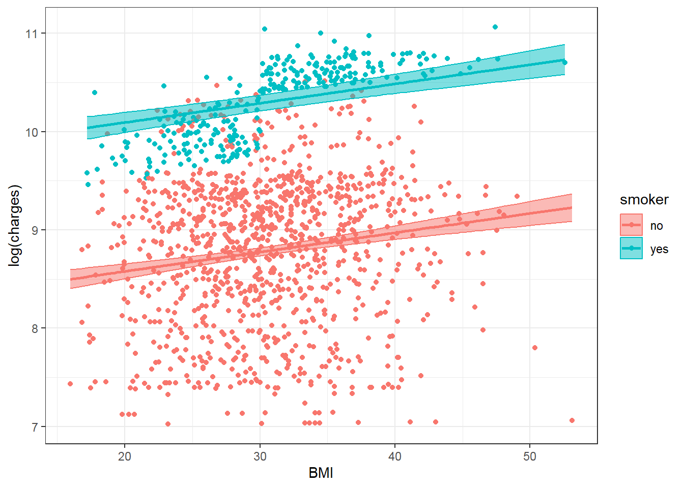

In the above multiple linear regression model with smoker and bmi as predictors, the slopes for logcharges against bmi is the same for smoker = no and smoker = yes. However, the above plot shows the difference in the association of logcharges against bmi between smoker = no and smoker = yes. Thus the multiple linear regression model above may not fit the data well, especially for smoker = yes.

To address this difference, an interaction term between smoker and bmi may be added to the model:

flm.i<-lm(logcharges ~ smoker + bmi +smoker*bmi, data=dlm)
sumflm.i<-summary(flm.i)
sumflm.i

## 
## Call:
## lm(formula = logcharges ~ smoker + bmi + smoker * bmi, data = dlm)
## 
## Residuals:
##      Min       1Q   Median       3Q      Max 
## -1.98216 -0.37399  0.07215  0.44881  1.72280 
## 
## Coefficients:
##               Estimate Std. Error t value Pr(>|t|)    
## (Intercept)   8.443124   0.106184  79.514  < 2e-16 ***
## smokeryes     0.342811   0.227399   1.508 0.131911    
## bmi           0.011259   0.003399   3.313 0.000949 ***
## smokeryes:bmi 0.038179   0.007259   5.259 1.68e-07 ***
## ---
## Signif. codes:  0 '***' 0.001 '**' 0.01 '*' 0.05 '.' 0.1 ' ' 1
## 
## Residual standard error: 0.6697 on 1334 degrees of freedom
## Multiple R-squared:  0.4708, Adjusted R-squared:  0.4696 
## F-statistic: 395.6 on 3 and 1334 DF,  p-value: < 2.2e-16

# Add confidence interval to summary
ciflm.i <- confint(flm.i)
sumciflm.i <- cbind(sumflm.i$coefficients, ciflm.i)
round(sumciflm.i, 4)

##               Estimate Std. Error t value Pr(>|t|)   2.5 % 97.5 %
## (Intercept)     8.4431     0.1062 79.5145   0.0000  8.2348 8.6514
## smokeryes       0.3428     0.2274  1.5075   0.1319 -0.1033 0.7889
## bmi             0.0113     0.0034  3.3126   0.0009  0.0046 0.0179
## smokeryes:bmi   0.0382     0.0073  5.2595   0.0000  0.0239 0.0524

And re-perform the plot:

predictions <- predict(flm.i, newdata=dlm, interval="confidence")
new_data <- cbind(dlm, as.data.frame(predictions))
#plot 
ggplot(new_data, aes(bmi, logcharges, color=smoker)) +
  geom_point() +
  geom_ribbon(data = new_data, aes(x = bmi, ymin = lwr, ymax = upr, fill=smoker), alpha = 0.5) +  
  geom_line(data = new_data, aes(bmi, fit, color=smoker), linewidth = 1) +
  labs(x = "BMI", y = "log(charges)") +
  theme_bw()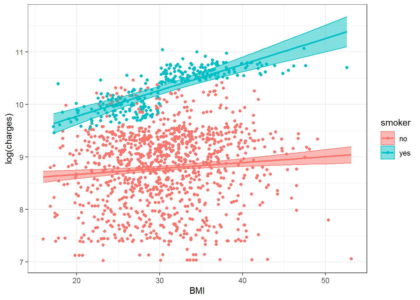

Now the plot shows two different slopes for smoker = no and smoker = yes and the model fits the data better especially for smoker = yes.

The interpretation of coefficients of the multiple linear regression model with interaction term is as below:

logcharges when smoker= no and bmi = 0 is 8.443124
When bmi = 0, logcharges when smoker= yes is is 0.3428113 higher when smoker= no
When smoker= no, for each unit increase in bmi, logcharges increases by 0.011259
Coefficient for interaction term expresses the change in a variable’s effect when the interacting variable is increased by one-unit:
- The effect of bmi on logcharges increases by 0.0381793 (logcharges per one unit of bmi) in smoker= yes vs smoker= no.
- For each unit increase in bmi, the effect of smoker= yes vs smoker= no on logcharges increases by 0.0381793.

The effect of bmi for smoker= yes or smoker= no may be calculated by adding the coefficient of bmi 0.011259 to the interaction coefficient, 0.0381793, multiplied by smoker as dummy variable 0, 1:

bmi.effect (smoker=no) = 0.011259 + 0.0381793 *0
bmi.effect (smoker=yes) = 0.011259 + 0.0381793 *1

The effect of smoker for any bmi may be calculated by adding the coefficient of smoker 0.3428113 to the interaction coefficient, 0.0381793and multiplied by bmi:

smoker.effect (bmi=15) = 0.3428113 + 0.0381793 *15

6.4 Reference materials

The following resources have been adapted for this chapter:

Introduction to Linear Regression in R by UCLA Office of Advanced Research Computing Statistical Methods and Data Analytics
Linear Regression Hands on R tutorial by Princeton University Library
How to Do Linear Regression in R by Datacamp
The dataset used in some examples of this chapter are example data regarding the association of medical costs and patient information: may be downloaded from Github.

References

Heinzen, Ethan, Jason Sinnwell, Elizabeth Atkinson, Tina Gunderson, and Gregory Dougherty. 2021. Arsenal: An Arsenal of r Functions for Large-Scale Statistical Summaries. https://github.com/mayoverse/arsenal.

———. 2024b. R: A Language and Environment for Statistical Computing. Vienna, Austria: R Foundation for Statistical Computing. https://www.R-project.org/.