Chapter 5 Basic Statistics with R

Hien Nguyen, PhD

Edited by: Nhan Thi Ho, MD, PhD

5.1 Theory of probability

5.1.1 Introduction

A statistical experiment, which gives one of several outcomes when repeated essentially under similar conditions, is called a trial. The outcomes of trials are called events, and the set of all possible outcomes is called the sample space. Events are said to be independent if the happening of an event is not affected by the happening of other events.

Example: Coin Toss

In the case of tossing a coin three timee,

• trial : tossing the coin
• number of trials : 3
• events : heads or tails obtained from 3 tosses (HHT, THT, …)
• number of possible outcomes: $2^3 = 8$
• events are independent

The probability $P$ of a favorable event $E$ wrt the sample space $S$ is given by

$$P(E) = \dfrac{|E|}{|S|}$$

Because $0 \leq |E| \leq |S|$, the range of $P(E)$ is $[0,1]$

• $P(E)$ is close to 0 => E is not likely to happen.
• $P(E)$ is close to 1 => E is very likely to happen.
• To compute $|S|$ and $|E|$, we use the rules of counting

Example: Powerball lottery

Ticket rule: Select five numbers from 1 to 69 for the white balls; then select one number from 1 to 26 for the red Powerball. The order among the white balls does not matter. What is the probability to win the Powerball lottery?

The number of possible tickets is:

$|S| = C(69, 5) * P(26, 1) = 292,201,338$

The probability to win is: 1/292,201,338.

Example: Poker

In poker, a hand of cards consists of 5 cards. What is the probability that a poker hand has four of a kinds?

The number of possible hands (|S|) is C(52, 5) = 2,598,960.

To get four of a kind, first pick a kind out of 13: P(13, 1) = 13. Then, pick the remaining card out of 48 cards left: P(48, 1) = 48

Number of possible four-of-a-kind hands: |E| = 13*48 = 624

The probability is P(E) = 624 / 2,598,960.

5.1.2 Some widely used laws

• $P(\bar{A}) = 1 - P(A)$
• $B \subset A \to P(B) \leq P(A)$
• $P(A \cup B) = P(A) + P(B) - P(A \cap B)$
• $P(A \cap B) = P(A)P(B)$, if A and B are independent
• $P(A \cap B) = P(A)P(B|A) = P(B)P(A|B)$, where $P(B|A)$ is the conditional probability occurrence of B when the event A has already occurred.

Example: Microarray experiments

In a microarray experiment, a spot is acceptable if it is either perfectly circular or perfectly uniform or both. In an experiment, a researcher found that there are a total of 20,000 spots. Out of these 20,000 spots, 15,500 are circular, 9,000 are uniform, and 5,000 spots are both circular and uniform. If a spot is chosen randomly, find the probability that the selected spot will be acceptable.

P(circular spot) = 15500/20000 = 0.775

P(uniform spot) = 9000/20000 = 0.45

P(circular and uniform spot) = 5000/20000 = 0.25

P(a randomly chosen spot is acceptable)

= P(circular) + P(uniform spot) - P(circular and uniform)

= 0.775 + 0.45 - 0.25 = 0.975

In a microarray experiment, a dye R will be labeled into target cDNA with a probability of 0.95. The probability that a signal will be read from a spot (labeled and hybridized) is 0.85. What is the probability that a labeled target cDNA hybridizes on a spot?

Answer: Let A be the event that the target cDNA will be labeled with the dye R. Let B be the event that the target cDNA will hybridize with the labeled dye R. If it is given that P(A) = 0.95, and P(A $\cap$ B) = 0.85, then the probability that the labeled target cDNA hybridizes on a spot is given by

$P(B|A) = \dfrac{P(A \cap B)}{P(A)} = \dfrac{0.85}{0.95} = 0.89$

5.1.3 Random variables

A random variable is a function that associates a real number with each element in the sample space. In other words, a random variable $X$ is a variable that enumerates the outcome of an experiment. Consider a trial of throwing two coins together. The sample space $S$ is {HH, HT, TH, TT}. If X is a random variable denoting the number of heads in this experiment, then the value of X can be shown as

Outcome	X
HH	2
HT	1
TH	1
TT	0

Let Y be a random variable denoting whether a gene being expressed or not, then

Y = 1, if the gene is expressed

Y = 0, if the gene is not expressed

5.1.4 Distribution function

The function $F(x) = P(X \leq x)$ is called the distribution function of $X$.

Properties of distribution functions

• $P(a < X \leq b) = F(b) - F(a)$
• $0 \leq F(x) \leq 1$
• $F(x) < F(y)$ if $x < y$

Discrete Random Variables

The probability distribution function (pdf) of a discrete random variable is called a probability mass function (pmf), denoted by $P(x_i)$, where $x_i$’s are the values of $X$. It satisfies:

• $P(x_i) \ge 0$
• $\sum_{i=1}^{\infty} P(x_i) = 1$

Continuous Random Variables

In a discrete probability function, sample space has either a finite or a countably infinite number of points. In contrast, in a continuous probability function, the sample space has an uncountably infinite number of points, which are spread over a real line or over some interval of the real line. It satisfies:

• $f(x) \ge 0$
• $\int_{S} f(x)dx = 1$

where $f(X)$ is the continuous density function of the random variable $X$. The distribution function is defined as

$$F(x) = P(X \leq x) = \int_{-\infty}^{x}f(t)dt$$

• $0 \leq F(x) \leq 1$
• $P(a \leq X \leq b) = \int_{-\infty}^{b}f(x)dx - \int_{-\infty}^{a}f(x)dx = F(b) - F(a)$

5.2 Special distributions

5.2.1 Binomial distribution

Consider a coin tossed $n$ times. Assume that each time, the probability for the head is $p$, and the probability for the tail is $1-p$.

The probability of $x$ successes and $(n-x)$ failures is given by

$$C(n, x) p^x (1-p)^{n-x}$$

since the $x$ successes in $n$ trials can occur in $C(n,x)$ ways.

A random variable $X$ is said to follow binomial distribution if its PDF is given by

$$P(X = x) = P(x) = \begin{cases} C(n, x) p^x (1-p)^{n-x} \text{, if x = 0,1,2,..,n}\\ 0 \text{, otherwise} \end{cases}$$

The two independent constants $n$ and $p$ are known as the parameters of the binomial distribution. The notation Bin(n, p) is used to denote that the random variable $X$ follows the binomial distribution with parameters $n$ and $p$. There are four defining conditions with the binomial distribution:

• Each trial results in one of the two possible outcomes.
• All trials in an experiment are independent.
• Probability of success is constant for all trials.
• The number of trials is fixed.

Using binomial distribution in R

# generate 100 values from a binomial distribution which has n = 40, p = 0.5
samp = rbinom(100, size = 40, prob = 0.5)
print(samp)

##   [1] 20 18 15 19 23 19 16 19 21 19 22 22 20 19 20 18 21 24 17 19 17 19 16 20 25 22 25 20 21 20 16 18
##  [33] 20 19 25 20 18 18 23 22 17 15 22 21 17 15 16 19 17 18 17 18 17 20 22 14 20 24 19 15 17 19 17 16
##  [65] 18 18 16 27 19 20 21 16 16 15 25 21 16 20 20 19 27 17 23 15 19 17 17 23 22 18 20 16 19 26 21 21
##  [97] 18 19 28 23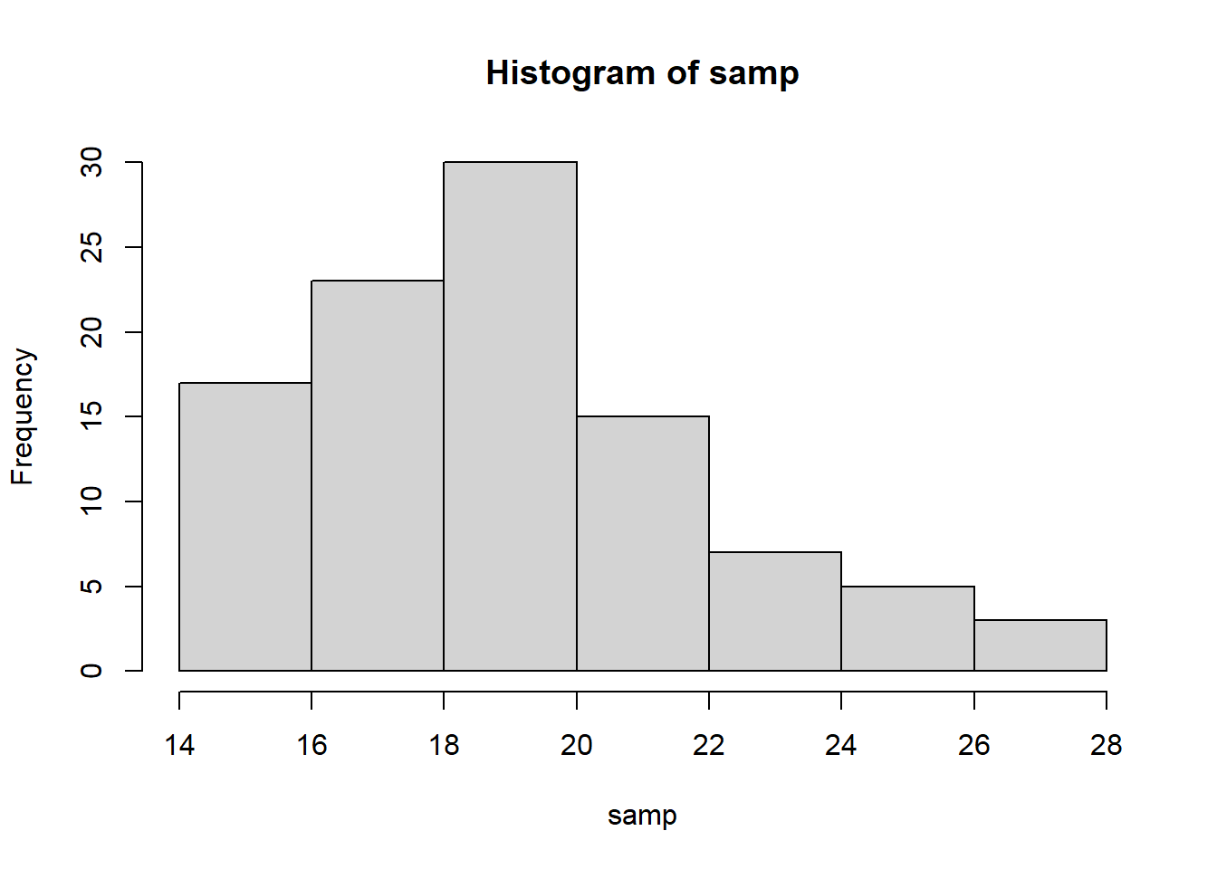

hist(samp)

# the probability function P(x <= 20)
pbinom(20, size = 40, prob = 0.5)

## [1] 0.5626853

# the density P(X = 20)
dbinom(20, size = 40, prob = 0.5)

## [1] 0.1253707

# the quantile function gives x such that P(X <= x) = 0.6
qbinom(0.6, size = 40, prob = 0.5)

## [1] 21

Example: Nucleotides

The DNA sequence of an organism consists of a long sequence of nucleotides adenine, guanine, cytosine, and thymine. It is known that in a very long sequence of 100 nucleotides, 22 nucleotides are guanine. In a sequence of 10 nucleotides, what is the probability that

1. exactly three nucleotides will be guanine?

2. at least four nucleotides will be guanine?

Answer:

The probability for a nucleotides to be a guanine $p = 22/100 = 0.22$.

The probability that out of 10 nucleotides, there will be x guanine is given by

$P(X = x) = C(10, x) 0.22^x(1-0.22)^{10-x}$

1. $P(X = 3) = C(10,3) 0.22^3 0.78^7 = 0.2244$

# a) compute P(X = 3), which is the density
dbinom(3, size = 10, prob = 0.22)

## [1] 0.2244458

# b) compute P(4) + P(5) + .. + P(10)
sum(dbinom(4:10, size = 10, prob = 0.22))

## [1] 0.1586739

# or
1 - pbinom(3, size = 10, prob = 0.22)

## [1] 0.1586739

5.2.2 Multinomial distribution

Multinomial distribution can be regarded as a generalization of binomial distribution when there are $k$ possible outcomes on each of $n$ independent trials.

The formula for binomial distribution can be rewritten as

$P(X = x_1) = \dfrac{n!}{x_1!x_2!}p_1^{x_1}p_2^{x_2}$

where $x_1 + x_2 = n$ and $p_1 + p_2 = 1$.

The formula for multinomial distribution is an extension:

$P(X_1 = x_1, X_2=x_2,..,X_k=x_k) = \dfrac{n!}{x_1!x_2!..x_k!}p_1^{x_1}p_2^{x_2}..p_k^{x_k}$

where $x_1 + x_2 +..+x_k = n$ and $p_1 + p_2 + .. + p_k = 1$.

Example: Induced mutation

In an induced mutation, mutation occurs as a result of treatment with a mutagenic agent such as ionizing radiation, nonionizing radiation, or a chemical substance. It is assumed that for a randomly selected gene, the mutation in the gene will occur due to ionizing radiation, nonionizing radiation, and chemical substance with respective probabilities 2/9, 1/5, and 26/45. What is the probability that out of seven randomly selected genes, two genes will have mutation due to ionizing radiations, two genes will have mutation due to nonionizing radiations, and three genes will have mutation due to chemicals?

Answer:

$x_1 = 2, x_2 = 2, x_3 = 3, p_1 = 2/9, p_2 = 1/5, p_3 = 26/45$

$P = \dfrac{7!}{2!2!3!}(2/9)^2(1/5)^2(26/45)^3 = 0.08$

dmultinom(x=c(2,2,3), prob=c(2/9,1/5,26/45))

## [1] 0.08000862

5.2.3 Normal distribution

A random variable $X$ is said to have a normal distribution with parameters $\mu$ and $\sigma^2$ if its density function is given by

$$f(x;\mu,\sigma) = \dfrac{1}{\sigma \sqrt{2\pi}}\exp\bigg[-\dfrac{(x-\mu)^2}{2\sigma^2}\bigg]$$ where $-\infty < x, \mu < \infty$, and $\sigma > 0$

Generally, it is denoted by $X \sim N(\mu,\sigma^2)$.

Then $Z = (x-\mu)/\sigma$ is a standard normal variate, $Z \sim N(0,1)$

Important Properties

• The curve is bell shaped and symmetrical about the line $x = \mu$.

• Mean, median, and mode of the distribution are the same.

• The linear combination of n independent normal variates is a normal variate.

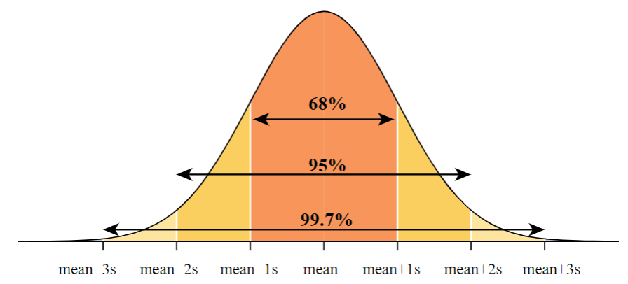
• Empirical rule: The probabilities of a point lying within $1\sigma$, $2\sigma$, and $3\sigma$ from the population mean are given by

  $P(\mu - \sigma < X < \mu + \sigma) = 0.6826$

  $P(\mu - 2\sigma < X < \mu + 2\sigma) = 0.9544$

  $P(\mu - 3\sigma < X < \mu + 3\sigma) = 0.9973$

• Most of the wellknown distributions such as binomial, Poisson, hypergeometric, and other distributions can be approximated by the normal distribution.

• Many sampling distributions such as the student’s t, Snedecor F, Chisquare distributions, etc., tend to normal distribution for large sample sizes.

• If a variable is not normally distributed, it may be possible to convert it into a normal variate using transformation of a variable.

• The entire theory of small sample tests-namely, t, F, and $\chi^2$ tests- is based on the assumption that the parent population from which samples are drawn is normal.

Example: progeny

Let the random variable $X$ denote the mutations among progeny of males that received a gamma radiation of 2500 roentgen (r) units. Let $X$ be normally distributed with a mean of 54 mutations per thousand and SD of 5 mutations per thousand.

1. Find the probability that the number of mutations among progeny of males will be more than 65.

2. Find the probability that the number of mutations among progeny of males will be between 47 and 62.

Answer:

Here $X \sim N(54, 5^2)$

# a. compute P(X > 65)
1 - pnorm(65, mean = 54, sd = 5)

## [1] 0.01390345

# b. compute P( 47 <= X <= 62)
pnorm(62, mean = 54, sd = 5) - pnorm(47, mean = 54, sd = 5)

## [1] 0.864444

Example: gene expression

Suppose that in a microarray experiment, a gene is said to be expressed if the expression level is between 500 and 600 units. It is supposed that gene expressions are normally distributed with mean 540 units and variance 252 units. What is the probability that a randomly selected gene from this population will be an expressed gene?

Answer:

Let X denote the expression level of a gene, $X \sim N(540, 25^2)$

# compute P(500 <= X <= 600)
pnorm(600, mean = 540, sd = 25) - pnorm(500, mean = 540, sd = 25)

## [1] 0.9370032

**Example: cDNA spots

Let the distribution of the mean intensities of cDNA spots, corresponding to expressed genes, be normal with mean 750 and standard deviation 502. What is the probability that a randomly selected expressed gene has a spot with a mean intensity

1. less than 825? _________________

2. more than 650? _________________

Normal approximation to the Binomial

If $X$ is a binomial random variable with mean $\mu = np$ and variance $\sigma^2 = np(1-p)$, then the limiting distribution of

$Z = \dfrac{X - np}{\sqrt{np(1-p)}}$

is the standard normal distribution $N(0, 1)$ as $n \to \infty$, and $p$ is not close to 0 or 1.

Let the probability that a gene has a rare gene mutation be 0.45. If 100 genes are randomly selected, use the normal approximation to binomial to find the probability that fewer than 35 genes will have the rare gene mutation.

Answer:

# Using binomial distribution to compute P(X <= 35)
pbinom(35, size = 100, prob = 0.45)

## [1] 0.0272363

# Using normal approximation to compute P(X <= 35)
mu = 100 * 0.45 - 0.5  # continuity correction
sigma = sqrt(100 * 0.45 * 0.55)
pnorm(35, mean = mu, sd = sigma )

## [1] 0.02809418

5.2.4 Chi-square distribution

If $X_i$ are $n$ independent normal variates with mean $\mu_i$, and variance $\sigma_i^2$, then

$\chi^2 = \sum\limits_{i=1}^n \big( \dfrac{X_i - \mu_i}{\sigma_i}\big)^2$

is a chi-square variable with $n$ degrees of freedom.

Properties

• If $X_1, X_2,.., X_k$ are independent chi-square variates with parameters $n_i$, $i = 1, 2,.., k$ then $X_1 + X_2 + .. + X_k$ is also a chi-square variate with $\sum n_i$ degrees of freedom.

• The chi-square distribution tends to the normal distribution for large degrees of freedom.

5.3 Basic statistical tests

5.3.1 Testing of hypotheses

We define a hypothesis as a statement about a population parameter. A simple hypothesis completely specifies the distribution, while a composite hypothesis does not completely specify the distribution. Thus, a simple hypothesis not only specifies the functional form of the underlying population distribution, but also specifies the values of all parameters. The hypothesis is further classified as a null hypothesis or an alternative hypothesis. The null and alternative hypotheses are complementary hypotheses.

Generally, the null hypothesis, denoted by $H_0$, is the claim that is initially assumed to be true. The null hypothesis can be considered as an assertion of “no change, effect, or consequence.” This suggests that the null hypothesis should have an assertion in which no change in situation, no difference in conditions, or no improvement is claimed. The alternative hypothesis is the assertion, denoted by $H_a$. For example, in the U.S. judicial system, a person is assumed to be innocent until proven guilty. This means that the null hypothesis is that the person is innocent, while the alternative hypothesis is that the person is guilty. The burden of proof is always on the prosecution to reject the null hypothesis (Zar 2010).

The form of the null hypothesis is given by

$H_0$ : population parameter or form = hypothesized value,

where the hypothesized value is specified by the investigator or the problem itself.

The alternative hypothesis can take one of the following three forms:

• $H_a$: population parameter > hypothesized value. This form is called one-sided alternative to right.
• $H_a$: population parameter < hypothesized value. This form is called one-sided alternative to left.
• $H_a$: population parameter $\neq$ hypothesized value. This form is called a two-sided alternative.

A test of hypotheses or test procedure is a method to decide whether the null hypothesis is rejected or accepted on the basis of the sample data.

The null hypothesis is rejected if and only if the numerical value of the test statistic, calculated on the basis of the sample, falls in the rejection region.

Usually, we calculate the $p$-value, which is a probability calculated using the test statistic. If the $p$-value is less than or equal to the predecided level of significance, then we reject the null hypothesis.

The $p$-value is defined as the probability of getting a value for the test statistic as extreme or more extreme than the observed value given that $H_0$ is true.

5.3.2 Tests about a Population Mean

5.3.2.1 Case I (Single sample case): Population is normal, $\sigma$ known, sample size is large.

In this case, the population standard deviation is known. Thus, we can use a $Z$-test, which is also known as a standardized test. The distribution of the $z$-statistic is normal.

Assumptions

The population is normal, population variance is known, and sample size is large.

Hypotheses

Null hypothesis $H_0 : \mu = \mu_0$.

Alternative hypotheses

$H_A : \mu < \mu_0$,

$H_A : \mu > \mu_0$,

$H_A : \mu \neq \mu_0$.

Test statistic

$Z = \dfrac{\bar{X} - \mu_0}{\sigma/\sqrt{n}}$

Rejection criteria

Choose one or both rejection criteria.

A. Critical value approach

• For $H_A : \mu < \mu_0$, reject the null hypothesis if $Z < -Z_\alpha$.
• For $H_A : \mu > \mu_0$, reject the null hypothesis if $Z > Z_\alpha$.
• For $H_A : \mu \neq \mu_0$, reject the null hypothesis if $Z < -Z_{\alpha/2}$ or $Z > Z_{\alpha/2}$.

B. p-value approach

Compute the $p$-value for the given alternative as follows:

• For $H_A : \mu < \mu_0$, $p = P(Z < -z)$.
• For $H_A : \mu > \mu_0$, $p = P(Z > z)$.
• For $H_A : \mu \neq \mu_0$, $p = 2P(Z > |z|)$.

Conclusion

Reject or accept the null hypothesis on the basis of the rejection criteria.

Example: Prokaryotic genome

Genes are organized in operons in the prokaryotic genome. The genes within an operon tend to have similar levels of expression. An experiment is conducted to find the true mean expression of an operon. The mean expression level of an operon consisting of 34 genes is found to be 0.20. Test the claim that the true mean expression of the population is 0.28 when the population variance is 0.14. Use the significance level as alpha = 0.05.

Answer:

Assumptions

The population is normal, population variance is known, and sample size is large.

Hypotheses

Null hypothesis $H_0 : \mu = \mu_0 = 0.28$.

Alternative hypotheses $H_A : \mu \neq 0.28$.

Test statistic

$Z = \dfrac{\bar{X} - \mu_0}{\sigma/\sqrt{n}} = \dfrac{0.2-0.28}{\sqrt{0.14}/\sqrt{34}} = -1.24$

Rejection criteria

A. Critical value approach

For $H_A : \mu \neq \mu_0$, since we have z = -1.24 > -$Z_{0.05/2}$ = -1.96, we fail to reject the null hypothesis

B. p-value approach

$p = 2P(Z > |z|) = 2*0.1075 = 0.215 > alpha$.

Therefore, we fail to reject the null hypothesis.

Conclusion

We fail to reject the null hypothesis. Thus, the true mean expression of the population is 0.28 when the population variance is 0.14.

xbar = 0.20
alpha = 0.05
varx = 0.14
n = 34
mu = 0.28
# compute z-statistic
z.score = (xbar - mu)/(sqrt(varx/n))
print(z.score)

## [1] -1.24671

# critical value approach, compute z critical
z.critical = qnorm(alpha/2, mean = 0, sd = 1)
print(z.critical)

## [1] -1.959964

# p-value approach
p = 2*pnorm(z.score, mean = 0, sd = 1)
print(p)

## [1] 0.2125039

5.3.2.2 Case II (Single sample case): Population is normal, $\sigma$ unknown, and the sample is small.

If the population standard deviation is unknown and the sample size is small, the z-test statistic no longer follows a standard normal distribution. In that case, we use another test called t-test, the procedure of which is as follows.

Assumptions

The population is normal, the population variance is unknown, and the sample size is small.

Hypotheses

Null hypothesis $H_0 : \mu = \mu_0$.

Alternative hypotheses

$H_A : \mu < \mu_0$,

$H_A : \mu > \mu_0$,

$H_A : \mu \neq \mu_0$.

Test statistic

$t = \dfrac{\bar{X}-\mu_0}{S/\sqrt{n}}$

with $v = n-1$ degrees of freedom.

Rejection criteria

Choose one or both rejection criteria.

A. Critical value approach

• For $H_A : \mu < \mu_0$, reject the null hypothesis if $t < -t_{\alpha,v}$.
• For $H_A : \mu > \mu_0$, reject the null hypothesis if $t > t_{\alpha,v}$.
• For $H_A : \mu \neq \mu_0$, reject the null hypothesis if $t < -t_{\alpha/2,v}$ or $t > t_{\alpha/2,v}$.

B. p-value approach

• For $H_A : \mu < \mu_0$, $p = P(T < -t)$.
• For $H_A : \mu > \mu_0$, $p = P(T > t)$.
• For $H_A : \mu \neq \mu_0$, $p = 2P(T > |t|)$.

Reject the null hypothesis if $p < \alpha$.

Conclusion

Reject or accept the null hypothesis on the basis of rejection criteria.

Example: Intertidal crabs

Consider the body temperatures of 25 intertidal crabs placed in air at 24.3 (Celsius). We ask whether the mean body temperature of this crab species is the same as the ambient air temperature.

$H_0: \mu = 24.3$

$H_A: \mu \neq 24.3$

dat = c(25.8, 24.6, 26.1, 22.9, 25.1, 27.3, 24.0, 24.5, 23.9, 26.2, 24.3, 24.6, 23.3, 25.5, 28.1, 24.8, 23.5, 26.3, 25.4, 25.5, 23.9, 27.0, 24.8, 22.9, 25.4)
t.test(dat, mu = 24.3)

## 
##  One Sample t-test
## 
## data:  dat
## t = 2.7128, df = 24, p-value = 0.01215
## alternative hypothesis: true mean is not equal to 24.3
## 95 percent confidence interval:
##  24.47413 25.58187
## sample estimates:
## mean of x 
##    25.028

5.3.2.3 Case III (Two-sample case): Populations are normal, population variances are known, sample sizes are large

The standard normal test for testing the difference in means can be used in this case. The distribution of Z-statistic is normal.

Assumptions

The two populations are normal, the population variances are known, and sample sizes are large.

Hypotheses

Let $\mu_1, \sigma_1, \mu_2, \sigma_2$ be the mean and the variance of population 1 and 2 respectively.

Null hypothesis: $\mu_1 - \mu_2 = \delta$ where $\delta$ is a constant

Alternative hypotheses

• $H_A : \mu_1 - \mu_2 < \delta$,
• $H_A : \mu_1 - \mu_2 > \delta$,
• $H_A : \mu_1 - \mu_2 \neq \delta$.

Test statistic

Let $x_1, x_2, n_1, n_2$ be the sample mean and the sample size from population 1 and 2. Then the test statistic is given by

$$Z = \dfrac{\bar{X_1} - \bar{X_2} - \delta}{\sqrt(\sigma_1^2/n_1+\sigma_2^2/n_2)}$$

Rejection criteria

Choose one or both rejection criteria.

A. Critical value approach

• $H_A : \mu_1 - \mu_2 < \delta$, reject the null hypothesis if $Z < -Z_\alpha$.
• $H_A : \mu_1 - \mu_2 > \delta$, reject the null hypothesis if $Z > Z_\alpha$.
• $H_A : \mu_1 - \mu_2 \neq \delta$, reject the null hypothesis if $Z < -Z_{\alpha/2}$ or $Z > Z_{\alpha/2}$.

B. p-value approach

Compute the p-value for the given alternative as follows:

• $H_A : \mu_1 - \mu_2 < \delta$, $p = P(Z < -z)$.
• $H_A : \mu_1 - \mu_2 > \delta$, $p = P(Z > z)$.
• $H_A : \mu_1 - \mu_2 \neq \delta$, $p = 2P(Z < |z|)$.

Reject the null hypothesis if $p < \alpha$ .

Conclusion

Reject or accept the null hypothesis on the basis of rejection criteria.

Example: DNA denaturation

The denaturation ofDNAoccurs over a narrow temperature range and results in striking changes in many of its physical properties. The midpoint of the temperature range over which the strands of DNA separate is called the melting temperature. The melting temperature may vary from species to species depending on the number of G and C base pairs contained in DNA.

To compare the melting temperature of two species A and B, two samples of sizes 34 and 45 were taken from species A and B, respectively. It was found that the mean temperatures of species are 82$^\circ$F and 85$^\circ$F for species A and B,respectively. The population standard deviations of species A and B were 12$^\circ$F and 14$^\circ$F, respectively. Test the claim that two species have the same mean melting temperature at alpha = 0.05.

Answer:

Assumptions

In this case, we assume that the two populations are normal. The population variances are known, and sample sizes are large.

Hypotheses

$H_0 : \mu_1 - \mu_2 = 0$ $H_A : \mu_1 - \mu_2 \neq 0$

Test statistic

We have $\sigma_1 = 12, \sigma_2 = 14, x_1 = 82, x_2 = 85, n_1 = 34, n_2 = 45$.

$$z = \dfrac{\bar{x_1}-\bar{x_2}}{\sqrt{\sigma_1^2/n_1 + \sigma_2^2/n_2}}= \dfrac{82-85}{\sqrt{12^2/34 + 14^2/45}}=-1.02$$

Rejection criteria

A. Critical value approach

For $H_A : \mu_1-\mu_2 \neq 0$, the $z_{\alpha/2} = z_0.025 = 1.96$.

Since z = -1.02 > -1.96, we fail to reject the null hypothesis.

B. p-value approach

For $H_A : \mu_1-\mu_2 \neq 0$, $p = 2P(Z > |z|) = 2(1-0.8461) = 0.3078$.

Since $p > \alpha$, we fail to reject the null hypothesis.

xbar = 82
ybar = 85
n1 = 34
n2 = 45
sdx = 12
sdy = 14
# compute z-score
z = (xbar - ybar)/(sqrt(sdx^2/n1 + sdy^2/n2))
print(z)

## [1] -1.023536

p = 2*(1-pnorm(abs(z)))
print(p)

## [1] 0.3060544

5.3.2.4 Case IV (Two-sample case): Population distribution is normal, $\sigma_1 = \sigma_2$ but unknown, sample sizes are small

Since the sample sizes are small, the standard normal test cannot be applied for this case. We can apply a t-test for the independent samples. The unknown variances are estimated by corresponding sample variances. The test statistic is the same as that of the Z-test for two samples, except that the distribution of the test statistic under the null hypothesis is a t-distribution with $n_1 + n_2 - 2$ degrees of freedom, and population variances are replaced by sample variances.

$$t=\dfrac{\bar{X_1}-\bar{X_2}-\delta}{S\sqrt{1/n_1+1/n_2}}$$ where $S^2 = \dfrac{(n_1-1)S_1^2+(n_2-1)S_2^2}{n_1+n_2-2}$

Rejection criteria

A. Critical value approach

• For $H_A : \mu_1-\mu_2 < \delta$, reject the null hypothesis if $t < -t_{\alpha,v}$.
• For $H_A : \mu_1-\mu_2 > \delta$, reject the null hypothesis if $t > t_{\alpha,v}$.
• For $H_A : \mu_1-\mu_2 = \delta$, reject the null hypothesis if $t < -t_{\alpha/2,v}$ or $t > t_{\alpha/2,v}$.

B. p-value approach

• For $H_A : \mu_1-\mu_2 < \delta, p = P(T < -t)$.
• For $H_A : \mu_1-\mu_2 > \delta, p = P(T > t)$.
• For $H_A : \mu_1-\mu_2 = \delta, p = 2P(T > |t|)$.

Reject the null hypothesis if $p < \alpha$.

Example: Mean number of ribosomes

One of the important functions in a cell is protein synthesis. To produce sufficient proteins, a cell uses many ribosomes contained in the cell. The number of proteins varies in different types of cells. Bacteria contain approximately 10,000 ribosomes. To test whether two species of bacteria have the same mean number of ribosomes, a sample size of 12 was drawn from each species. It was found that the sample mean and sample standard deviation of species 1 are 10,500 and 25, respectively, while for species 2, the sample mean and standard deviation are 10,512, and 50, respectively. Test whether the mean number of ribosomes is the same in two species. Use a 5% level of significance. Assume that the populations under consideration are normally distributed and population variances are unknown but equal (Mathur 2009).

Answer:

Compute t-statistic and the corresponding p-value, which gives p-value = 0.465. We fail to reject the null hypothesis.

xbar = 10500
ybar = 10512
n1 = 12
n2 = 12
df = n1+n2-2
s1 = 25
s2 = 50
s = sqrt(((n1-1)*s1^2 + (n2-1)*s2^2)/df)
t = (xbar - ybar)/(s*sqrt(1/n1+1/n2))
p = 2*(1-pt(abs(t), df))
print(p)

## [1] 0.4649789

Example: blood-clotting time

Adult male rabbits were divided at random into two groups, one group of six and one group of seven. The members of the first group were given drug B, and the members of the second group were given drug G. Blood is to be taken from each rabbit and the time (in minutes) it takes the blood to clot is to be recorded.

Given drug B: 8.8, 8.4, 7.9, 8.7, 9.1, 9.6 Given drug G: 9.9, 9.0, 11.1, 9.6, 8.7, 10.4, 9.5

x = c(8.8, 8.4, 7.9, 8.7, 9.1, 9.6)
y = c(9.9, 9.0, 11.1, 9.6, 8.7, 10.4, 9.5)
t.test(x, y)

## 
##  Welch Two Sample t-test
## 
## data:  x and y
## t = -2.5454, df = 10.701, p-value = 0.02774
## alternative hypothesis: true difference in means is not equal to 0
## 95 percent confidence interval:
##  -1.8543048 -0.1314095
## sample estimates:
## mean of x mean of y 
##  8.750000  9.742857

Conclusion: _________________

5.3.2.5 Nonparametric tests

There is a large body of statistical methods that do not require the estimation of population parameters (such as $\mu$ and $\sigma$) and that test hypotheses that are not statements about population parameters. These statistical procedures are termed nonparametric tests. These are in contrast to procedures such as t-tests, which are called parametric tests and which do rely upon estimates of population parameters and upon the statement of parameters in the statistical hypotheses. Although they may assume that the sampled populations have the same dispersion or shape, nonparametric methods typically do not make assumptions about the nature of the populations’ distributions (e.g., there is no assumption of normality); thus they are sometimes referred to as distribution-free tests. Both parametric and nonparametric tests require that the data have come at random from the sampled populations.

One-sample Wilcoxon test

Example of Intertidal Crabs revisited:

dat = c(25.8, 24.6, 26.1, 22.9, 25.1, 27.3, 24.0, 24.5, 23.9, 26.2, 24.3, 24.6, 23.3, 25.5, 28.1, 24.8, 23.5, 26.3, 25.4, 25.5, 23.9, 27.0, 24.8, 22.9, 25.4)
wilcox.test(dat, mu = 24.3)

## 
##  Wilcoxon signed rank test with continuity correction
## 
## data:  dat
## V = 232.5, p-value = 0.01908
## alternative hypothesis: true location is not equal to 24.3

Two-sample Wilcoxon test

Also known as Mann-Whitney test

Example of Blood Clotting revisited:

x = c(8.8, 8.4, 7.9, 8.7, 9.1, 9.6)
y = c(9.9, 9.0, 11.1, 9.6, 8.7, 10.4, 9.5)
wilcox.test(x, y)

## 
##  Wilcoxon rank sum test with continuity correction
## 
## data:  x and y
## W = 7, p-value = 0.05313
## alternative hypothesis: true location shift is not equal to 0

5.4 Basic sample size and power calculation

5.4.1 One-sample testing

5.4.1.1 Confidence intervals for the population mean

To reject a null hypthesis with $\alpha = 0.05$, we check if $|t| > t_{0.025, v}$, that is, $P(|t| \leq t_{0.025, v}) = 0.95$.

Let $S_{\bar{X}}$ denote $S/\sqrt{n}$, it follows that

$P(-t_{0.025, v} \leq \dfrac{\bar{X}-\mu}{S_{\bar{X}}} \leq t_{0.025, v}) = 0.95$

and

$P(\bar{X}-t_{0.025, v}S_{\bar{X}} \leq \mu \leq \bar{X} + t_{0.025, v}S_{\bar{X}}) = 0.95$

The value of the population mean $\mu$ is unknow, but we estimate it as $\bar{X}$. And if we have many samples, then 95% of the samples will have $\mu$ in the interval $[\bar{X}-t_{0.025, v}S_{\bar{X}} , \bar{X} + t_{0.025, v}S_{\bar{X}} ]$. This interval is called confidence interval (CI) for $\mu$.

In general, $P(\bar{X}-t_{\alpha/2, v}S_{\bar{X}} \leq \mu \leq \bar{X} + t_{\alpha/2, v}S_{\bar{X}}) = 1-\alpha$

5.4.1.2 Sample size and the estimation of the population mean

Question: How large a sample must be taken to achieve a desired precision in estimating the mean of a population ?

It’s obvious that narrower CI is more desirable than wider CI. If the CI is $\bar{X} \pm d$, where $d = t_{0.025, v}S_{\bar{X}}$, then

$d = t_{0.025, v}S/\sqrt{n}$, which leads to $n=\dfrac{S^2t^2_{0.025,v}}{d^2}$

Determine the sample size by Approximation

If we specify that we wish to estimate $\mu$ with a 95% CI no wider than 0.5, then $d=0.25$. Assume that $\alpha =0.05$, and $S^2 = 0.4008$ for this example.

Let’s guess that a sample of 40 is necessary, then $t_{0.025,39} = 2.023$

$n = \dfrac{0.4008*2.023^2}{0.25^2} = 26.2 \sim 27$

Repeat the estimation for $n$, now with $t_{0.025,26} = 2.056$:

$n = \dfrac{0.4008*2.056^2}{0.25^2} = 27.1 \sim 27$

The value of $n$ converged, we conclude that a sample size greater than 27 is required to achieve the specified CI.

5.4.1.3 Sample size required

We may specify that we wish to perform a t-test with a probability of $\alpha$ of committing a Type I error and a probability of $\beta$ of committing a Type II error; and we can state that we want to be able to detect a difference between $\mu$ and $\mu_0$ as small as $\delta$ (where $\mu$ is the actual population mean and $\mu_0$ is the mean specified in the null hypothesis). To test at the a significance level with $1-\beta$ power, the minimum sample size required to detect $\delta$ is

$n = \dfrac{S^2}{\delta^2}(t_{\alpha,v}+t_{\beta,v})^2$

Example:

Given $\alpha = 0.05, 1-\beta = 90\%, S^2= 1.5682$, how large is the sample needed to reject the null hypothesis if we wish to detect the population mean different from $\mu_0 = 0$ by as little as 1.0.

alpha = 0.05
beta = 0.1
S = sqrt(1.5682)
delta = 1.0
pwr.t.test(d = delta/S, sig.level = alpha, power = 1-beta, type="one.sample")

## 
##      One-sample t test power calculation 
## 
##               n = 18.50579
##               d = 0.7985448
##       sig.level = 0.05
##           power = 0.9
##     alternative = two.sided

5.4.1.4 Minimum detectable difference

By rearranging the formula, we can ask how small a $\delta$ can be detected by the t-test with the given power, the level of significance, and the sample size.

$\delta = \dfrac{S}{\sqrt{n}}(t_{\alpha,v}+t_{\beta,v})$

alpha = 0.05
beta = 0.1
S = sqrt(1.5682)
n = 25
d=pwr.t.test(n = n, sig.level = alpha, power = 1-beta, type="one.sample")$d
delta = d*S
print(delta)

## [1] 0.8464205

5.4.1.5 Power

If our desire is to express the probability of correctly rejecting a false $H_0$ about $\mu$, then we seek to estimate the power of a t-test.

$t_{\beta,v} = \dfrac{\delta\sqrt{n}}{S} - t_{\alpha,v}$

alpha = 0.05
S = sqrt(1.5682)
n = 15
delta = 1.0
pwr.t.test(n = n, d = delta/S,  sig.level = alpha,  type="one.sample")

## 
##      One-sample t test power calculation 
## 
##               n = 15
##               d = 0.7985448
##       sig.level = 0.05
##           power = 0.8199455
##     alternative = two.sided

5.4.2 Two-sample testing

5.4.2.1 Confidence Intervals

In two-sampe t-test, the 95% CI for $\mu$ is given as

$\bar{X_p} \pm t_{\alpha/2,v}\dfrac{S_p}{\sqrt{n_1+n_2}}$

It follows that

$n = \dfrac{2S_P^2t^2_{\alpha/2,v}}{d^2}$

It is best to have equal sample sizes $(n_1=n_2$, but it is not always practical. If $n_1$ is constrained, then we compute $n_2$ as

$n_2 = \dfrac{nn_1}{2n_1-n}$

5.4.2.2 Sample size required

Example: blood clotting revisited

From the data, we compute $S^2= 0.52$. We wish to detect a true difference between population mean as small as 0.5.

alpha = 0.05
S = sqrt(0.52)
beta = 0.1
delta = 0.5
pwr.t.test( d = delta/S,  sig.level = alpha, power=1-beta, type="two.sample")

## 
##      Two-sample t test power calculation 
## 
##               n = 44.69342
##               d = 0.6933752
##       sig.level = 0.05
##           power = 0.9
##     alternative = two.sided
## 
## NOTE: n is number in *each* group

5.4.2.3 Minimum detectable difference

Rearrange the formula to get

$\delta \ge \sqrt{\dfrac{2S_p^2}{n}}(t_{\alpha,v} + t_{\beta,v})$

Suppose n = 20, what size difference betweens means do we have a 90% chance to detect ?

alpha = 0.05
S = sqrt(0.52)
beta = 0.1
n = 20
d = pwr.t.test(n = n, sig.level = alpha, power=1-beta, type="two.sample")$d
delta = d*S
print(delta)

## [1] 0.7586061

5.4.2.4 Power

Rearrange the formulat to get $t_{\beta,v}$

$t_{\beta,v} \leq \dfrac{\delta\sqrt{n}}{\sqrt{2S^2_p}}-t_{\alpha/2,v}$

What would be the probability of detecting a true difference of 1.0 minute between mean blood-clotting of persons using the two drugs, if $n_1 = n_2=15$ and $\alpha = 0.05$ ?

alpha = 0.05
S = sqrt(0.52)
delta = 1.0
n = 15
pwr.t.test(n = n, d= delta/S, sig.level = alpha, type="two.sample")

## 
##      Two-sample t test power calculation 
## 
##               n = 15
##               d = 1.38675
##       sig.level = 0.05
##           power = 0.9558659
##     alternative = two.sided
## 
## NOTE: n is number in *each* group

5.5 Reference materials

The following resources have been adapted for this chapters:

• Statistical Bioinformatics with R, by Sunil Mathur
• Biostatistical Analysis, by Jerrold Zar

References

Mathur, Sunil K. 2009. Statistical Bioinformatics with r. 1st ed. Elsevier.

Zar, Jerrold H. 2010. Biostatistical Analysis. 5th ed. Prentice Hall.