Chapter 11 Special topic: Statistical analysis and meta-analysis of microbiome data with metamicrobiomeR package
Nhan Thi Ho, MD, PhD
11.1 Introduction
The metamicrobiomeR package was developed by Nhan Thi Ho, the editor and primary author of this book. During her research project at Columbia University Medical Center regarding meta-analysis of effects of exclusive breastfeeding on infant gut microbiome across populations, many difficulties arose. First, there was a lack of statistical method for proper analysis of zero-inflated compositional microbiome relative abundance data. Second, available methods for differential analysis of microbiome data did not produce standardized effect estimates that might be pooled across studies for meta-analysis. To address this gap, she implemented Generalized Additive Model for Location, Scale and Shape (GAMLSS) with zero inflated beta (BEZI) family for analysis of microbiome relative abundance data with various options for data transformation/normalization to address compositional effects. Moreover, the differential effect estimates using this method may be pooled across studies for meta-analysis. The metamicrobiomeR package is the implementation of these approaches together with some other related functions for microbiome data analysis, meta-analysis and visualization. The paper describing the metamicrobiomeR package may be found on BMC Bioinformatics (N. T. Ho et al. 2019). The package is hosted in R cran and an earlier version with full package tutorial may be found on Github.
11.2 Statistical approaches
The R package metamicrobiomeR applies Generalized Additive Models for Location, Scale and Shape (GAMLSS) with a zero-inflated beta (BEZI) family (GAMLSS-BEZI) for the analysis of microbial taxonomy relative abundance data. GAMLSS is a general framework for fitting regression type models in which the response variable can be any distribution (Rigby and Stasinopoulos 2005). With BEZI family, this model allows direct and proper examination of microbiome relative abundance data, which resemble a zero-inflated beta distribution. In principle, this model is similar to the two-part mixed effect model proposed by Chen et al (E. Z. Chen and Li 2016) in that the presence/absence of the taxon in the samples is modeled with a logistic component and the non-zero abundance of the taxon is modeled with a Beta component. Both logistic and beta components allow covariate adjustment and address longitudinal correlations with subject-specific random effects. The GAMLSS-BEZI is based on the broadly applicable established GAMLSS framework that can be flexibly implemented and applied to different types of data and study designs (e.g. cross-sectional and longitudinal) as in the taxa.compare functions. Importantly, the estimates (regression coefficients) from GAMLSS-BEZI are log (odds ratio) of being in the case group (as compared to being in the control group) with changes in relative abundance of a specific bacterial taxon and thus are analogous across microbiome studies and can be directly combined using standard meta-analysis approaches. As such, random effects or fixed effects meta-analysis models may be applied to pool the estimates and standard errors as implemented in meta.taxa functions of the metamicrobiomeR package. This approach allows examination of study-specific effects, heterogeneity between studies, and the overall pooled effects across studies. In the taxa.compare function, all bacterial taxa or pathway data are first filtered to retain features with mean relative abundance ≥ relative abundance threshold (e.g. ≥0.005%) and with prevalence ≥ prevalence threshold (e.g. present in ≥5% of the total number of samples). This pre-filtering step has been shown to improve performance of various differential abundance detection strategies (McMurdie and Holmes 2014). A filtered data matrix is then modeled by GAMLSS-BEZI and (μ) logit link and other default options using the R package ‘gamlss’ version 5.0–5 (Rigby and Stasinopoulos 2005). For longitudinal data, subject-specific random effects can be added to the model. The default implementation is subject random intercepts as in practice this is often sufficient to address the longitudinal correlations (Min and Agresti 2005). However, it is possible to extend the model to include random slopes depending on the specific research content. In addition, different approaches to deal with compositional effects are also implemented including Centered Log Ratio (CLR) transformation (Aitchison et al. 2000) with various zero-replacement options (Palarea-Albaladejo and Martin-Fernandez 2015) and Geometric Mean of Pairwise Ratios (GMPR) normalization (L. Chen et al. 2018). Multiple testing adjustment can be done using different methods (False Discovery Rate (FDR) control by default). For more detailed description of statistical approaches and demonstration, please see the package paper at BMC Bioinformatics (N. T. Ho et al. 2019).
11.3 Example data
For differential relative abundances analysis, the example dataset are published data from a cohort study of 50 healthy Bangladeshi infants, which included longitudinal gut microbiome data from 996 stool samples collected monthly from birth to 2 years of life (Subramanian et al. 2014). This study included longitudinal monthly data regarding the infants’ breastfeeding practices (exclusive, non-exclusive), duration of exclusive breastfeeding, infant age (months) at solid food introduction, and occurrence of diarrhea around the time of stool sample collection. A subset of samples collected around birth are used as example cross-sectional dataset (50 samples) and data from all samples are used as a longitudinal dataset (996 samples). For metaanalysis, gut microbiome data from four published studies are used to demonstrate the application of random effects models for meta-analysis across microbiome studies. These four studies include:
- a cohort of healthy infants in Bangladesh (Subramanian et al. 2014) (the data of this study was also used in the examples demonstrating the use of GAMLSS-BEZI with taxa.compare function);
- a cross-sectional study of Haiti infants negative for HIV who were exposed or unexposed to maternal HIV (Bender et al. 2016);
- a cohort of healthy infants in the USA (California and Florida [CA_FL]) (Pannaraj et al. 2017); and
- a small cohort of healthy infants in the USA (North Carolina [NC]) (Thompson et al. 2015).
More details about the four studies included in the meta-analysis are described in the package paper.
11.4 metamicrobiomeR package summary
The metamicrobiomeR package includes the functions below:
| Functions | Description |
|---|---|
| taxa.filter | Filter relative abundances of bacterial taxa or pathways using prevalence and abundance thresholds |
| taxa.meansdn | Summarize mean, standard deviation of abundances and number of subjects by groups for all bacterial taxa or pathways |
| taxa.mean.plot | Plot mean abundance by groups (from taxa.meansdn output) |
| taxa.compare | Compare relative abundances of bacterial taxa at all levels using GAMLSS or linear/linear mixed effect models (LM) or linear/linear mixed effect models with arcsin squareroot transformation (LMAS) |
| pathway.compare | Compare relative abundances of bacterial functional pathways at all levels using GAMLSS or LM or LMAS. Compare of log(absolute abundances) of bacterial functional pathways at all levels using LM |
| taxcomtab.show | Display the results of relative abundance comparison (from taxa.compare or pathway.compare outputs) |
| meta.taxa | Perform meta-analysis of relative abundance estimates of bacterial taxa or pathways (either from GAMLSS or LM or LMAS) across studies (from combined taxa.compare/pathway.compare outputs of all included studies) using random effect and fixed effect meta-analysis models |
| metatab.show | Display meta-analysis results of bacterial taxa or pathway relative abundances (from meta.taxa output) |
| meta.niceplot | Produce nice combined heatmap and forest plot for meta-analysis results of bacterial taxa and pathway relative abundances (from metatab.show output) |
| read.multi | Read multiple files in a path to R |
| alpha.compare | Calculate average alpha diversity indexes for a specific rarefaction depth, standardize and compare alpha diversity indexes between groups |
| microbiomeage | Predict microbiome age using Random Forest model based on relative abundances of bacterial genera shared with the Bangladesh study |
11.5 Package usage
This is a short, simplified version of the package tutorial. Only illustration and examples for the analysis of differential relative abundance using GAMLSS-BEZI and meta-analysis across studies using random effects models are shown. Full illustration, examples of all implemented functions, workflows and data are available at the package github repo. A simplified version of package vignette is also available in R cran. Install and load metamicrobiomeR and other required packages:
11.5.1 Example differential analysis: Comparison between breastfeeding statuses in infants < 6 months of age
In the example data, relative abundances of bacterial taxa at various taxonomic levels (from phylum to genus or species) are obtained via the summarize_taxa.py script in QIIME1 (Caporaso et al. 2010). Bacterial functional pathway abundances (e.g. Kyoto Encyclopedia of Genes and Genomes (KEGG) pathway level 1 to 3) are obtained from metagenome prediction analysis using PICRUSt (Langille et al. 2013). The relative abundance data should first be filtered with taxa.filter function. Then the function taxa.meansdn is used to summarize the mean, standard deviation of abundances and number of subjects by groups for all bacterial taxa of all levels or for pathways by comparison and grouping variables. Then the function taxa.mean.plot is used to visualize data summary for selected taxonomic level as in the example codes and figure. The values to be displayed in the figure may be filtered by mean.filter option and taxonomic level names may be displayed as short or full long names via option show.taxname.
11.5.1.1 Plot of mean relative abundance by breastfeeding statuses and age at phylum level:
data(taxtab6)
taxlist.rm<-taxa.filter(taxtab=taxtab6,percent.filter = 0.05, relabund.filter = 0.00005)
taxa.meansdn.rm<-taxa.meansdn(taxtab=taxtab6,sumvar="bf",groupvar="age.sample")
taxa.meansdn.rm<-taxa.meansdn.rm[taxa.meansdn.rm$bf!="No_BF",]
taxa.meansdn.rm$bf<-gdata::drop.levels(taxa.meansdn.rm$bf,reorder=FALSE)
#phylum
p.bf.l2<-taxa.mean.plot(tabmean=taxa.meansdn.rm,tax.lev="l2", comvar="bf", groupvar="age.sample",mean.filter=0.005, show.taxname="short")
p.bf.l2$p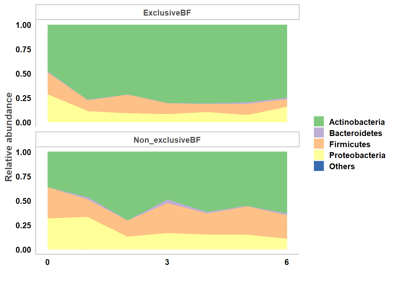
At family level:
p.bf.l5<-taxa.mean.plot(tabmean=taxa.meansdn.rm,tax.lev="l5", comvar="bf", groupvar="age.sample",mean.filter=0.005, show.taxname="short")
p.bf.l5$p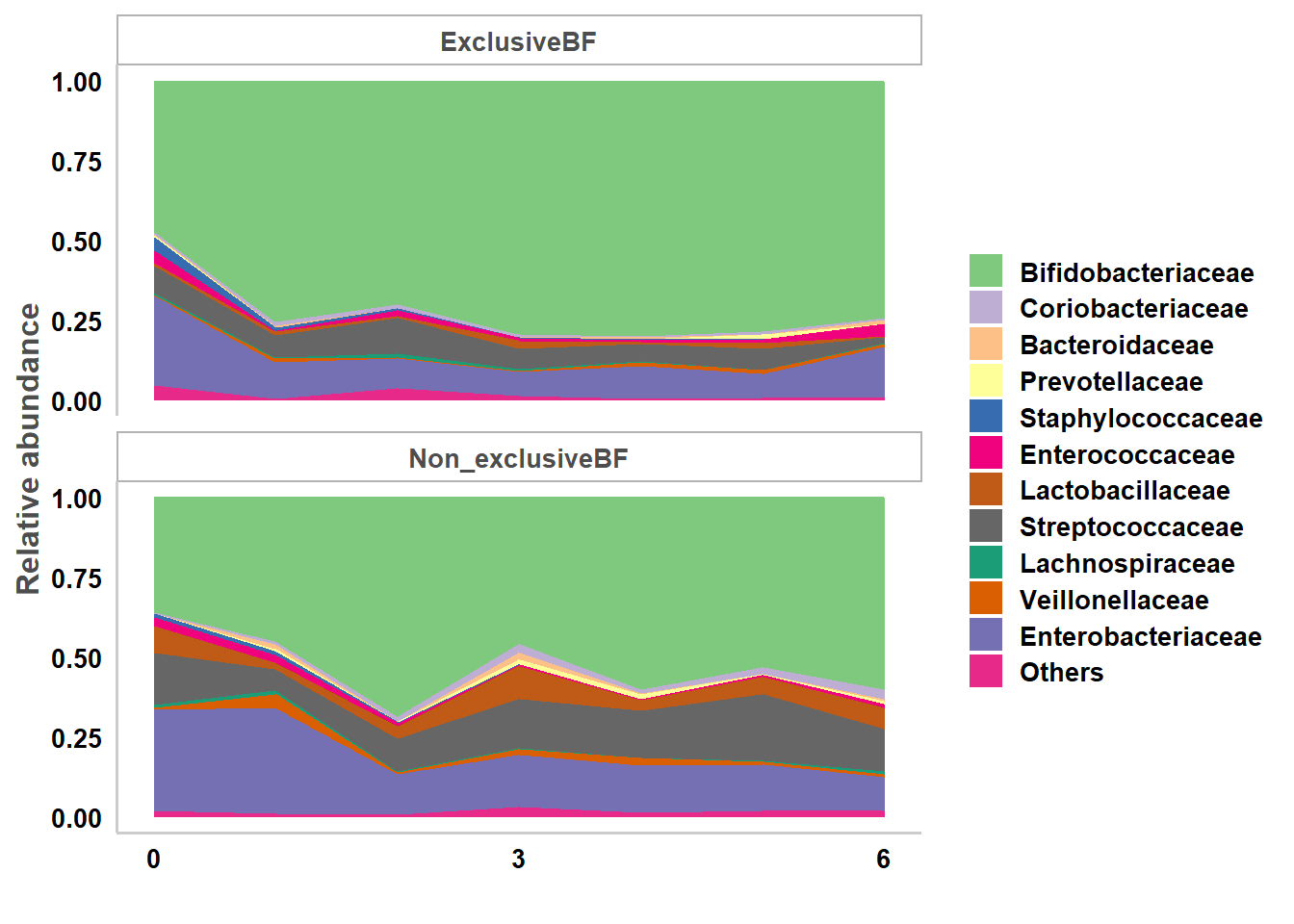
11.5.1.2 Comparison of taxonomic data between groups using GAMLSS-BEZI
Taxa.compare and pathway.compare are basically similar. There are just some adjustment to make these two functions readily to be used with different data format for pathway and taxonomy data. Various statistical methods for differential analysis of relative abundance data may be selected by propmed.rel with default= “gamlss”. Various data transformation may be selected by transform with default= “none”. Various methods for zero replacement may be selected by zeroreplace.method with default = “none”. The data may be filtered before differential analysis by setting filter threshold for prevalence with percent.filter and for relative abundance with relabund.filter. If the data is longitudinal, select the option longitudinal = “Yes”. Various options for adjusting for multiple testing may be selected via option p.adjust.method with default = “fdr”.
Example comparison between breastfeeding statuses adjusting for age of infants at sample collection:
Note: running time is not long in regular laptop for both GAMLSS-BEZI analysis (~10s) and meta-analysis (~5s). However, to save running time, only taxonomies of one phylum are selected for differential analysis example.
tab6<-as.data.frame(taxtab6)
tl<-colnames(taxtab6)[grep("k__bacteria.p__fusobacteria",colnames(taxtab6))]
taxacom.ex<-taxa.compare(taxtab=tab6[,c("personid","x.sampleid","bf","age.sample",tl)],propmed.rel="gamlss",comvar="bf",adjustvar="age.sample",
longitudinal="yes",p.adjust.method="fdr")
The result output from the taxa.compare function may be displayed using taxcomtab.show function. The taxa level to be displayed me be selected by tax.lev with options from “l2” (phylum) to “l7” (species) and the default is “l2”. Options for multiple testing re-adjustment for only the level to be displayed or keeping original multiple testing adjustment for all taxa of all levels may be selected with readjust.p.
Display phylum level:
tp<-taxcomtab.show(taxcomtab=taxacom.ex,tax.select="none", showvar="bfNon_exclusiveBF", tax.lev="l2",readjust.p=TRUE,p.adjust.method="fdr",p.cutoff = 1)
tp
## id Estimate.bfNon_exclusiveBF ll ul Pr(>|t|).bfNon_exclusiveBF
## 1 k__bacteria.p__fusobacteria -0.06 -0.77 0.65 0.87
## pval.adjust.bfNon_exclusiveBF
## 1 0.87Display genus level:
tp<-taxcomtab.show(taxcomtab=taxacom.ex,tax.select="none", showvar="bfNon_exclusiveBF", tax.lev="l6",readjust.p=TRUE,p.adjust.method="fdr",p.cutoff = 1)
head(tp)
## id
## 5 k__bacteria.p__fusobacteria.c__fusobacteriia.o__fusobacteriales.f__fusobacteriaceae.g__fusobacterium
## Estimate.bfNon_exclusiveBF ll ul Pr(>|t|).bfNon_exclusiveBF pval.adjust.bfNon_exclusiveBF
## 5 -0.12 -0.95 0.72 0.785 0.78511.5.1.3 Comparison taxonomic data between groups using Linear model with arcsin squareroot transformation (LMAS)
This approach was formerly used with MaAsLin by The Huttenhower Lab. This is also implemented in the metamicrobiomeR package for comparison and demonstration of the advantage of the GAMLSS-BEZI approaches for microbiome relative abundance data. Comparison of taxonomic data between breastfeeding statuses adjusting for age of infants at sample collection and display results of phylum and family levels:
taxacom.lmas<-taxa.compare(taxtab=tab6[,c("personid","x.sampleid","bf","age.sample",tl)], propmed.rel="lm",transform="asin.sqrt",comvar="bf",adjustvar="age.sample", longitudinal="yes",p.adjust.method="fdr")
#phylum
ts<-taxcomtab.show(taxcomtab=taxacom.lmas,tax.select="none", showvar="bfNon_exclusiveBF", tax.lev="l2",readjust.p=TRUE,p.adjust.method="fdr",p.cutoff = 1, digit=5,p.digit=5)
ts
## id Estimate.bfNon_exclusiveBF ll ul Pr(>|t|).bfNon_exclusiveBF
## 1 k__bacteria.p__fusobacteria 0.00134 -0.00134 0.00402 0.321
## pval.adjust.bfNon_exclusiveBF
## 1 0.321#family
ts<-taxcomtab.show(taxcomtab=taxacom.lmas,tax.select="none", showvar="bfNon_exclusiveBF", tax.lev="l5",readjust.p=TRUE,p.adjust.method="fdr",p.cutoff = 1, digit=5,p.digit=5)
head(ts)## id
## 4 k__bacteria.p__fusobacteria.c__fusobacteriia.o__fusobacteriales.f__fusobacteriaceae
## Estimate.bfNon_exclusiveBF ll ul Pr(>|t|).bfNon_exclusiveBF
## 4 0.00137 -0.00131 0.00405 0.31
## pval.adjust.bfNon_exclusiveBF
## 4 0.3111.5.1.4 Comparison of bacterial functional (KEGG) pathways between groups
The approach in pathway.compare is similar as that in taxa.compare function except some adjustment for data format obtained from metagenome prediction analysis using PICRUSt (Langille et al. 2013).
Example comparison of relative abundance of bacterial functional (KEGG) pathways between male vs. female infants < 6 months adjusting for breastfeeding statuses and age of infants at sample collection:
Example comparison of pathway relative abundances for level 1 only (to save running time).
data(kegg.12)
data(covar.rm)

path1<-pathway.compare(pathtab=kegg.12,mapfile=covar.rm,sampleid="sampleid", pathsum="rel",stat.med="gamlss",comvar="gender",adjustvar=c("age.sample","bf"), longitudinal="yes",p.adjust.method="fdr",percent.filter=0.05,relabund.filter=0.00005)
Show results of KEGG pathway level 1 and level 2:
#Level 1
tk<-taxcomtab.show(taxcomtab=path1$l1, sumvar="path", tax.lev="l2",tax.select="none",showvar="genderMale", p.adjust.method="fdr",p.cutoff=1)
tk
## id Estimate.genderMale ll ul Pr(>|t|).genderMale
## 7 Organismal.Systems 0.04 0.02 0.06 0.0000
## 5 Metabolism 0.01 0.00 0.01 0.0155
## 4 Human.Diseases -0.02 -0.03 0.00 0.0273
## 8 Unclassified -0.01 -0.02 0.00 0.0521
## 2 Environmental.Information.Processing -0.01 -0.02 0.00 0.1705
## 3 Genetic.Information.Processing 0.01 0.00 0.01 0.2454
## 6 None -0.06 -0.16 0.05 0.2877
## 1 Cellular.Processes 0.00 -0.03 0.02 0.8100
## pval.adjust.genderMale
## 7 0.0001
## 5 0.0619
## 4 0.0727
## 8 0.1043
## 2 0.2728
## 3 0.3271
## 6 0.3288
## 1 0.8100#Level 2
tk<-taxcomtab.show(taxcomtab=path1$l2, sumvar="path", tax.lev="l2",tax.select="none",showvar="genderMale", p.adjust.method="fdr",p.cutoff=1)
head(tk)## id Estimate.genderMale ll ul
## 36 Cellular.Processes..Transport.and.Catabolism 0.07 0.04 0.10
## 9 Organismal.Systems..Endocrine.System 0.09 0.05 0.12
## 2 Metabolism..Biosynthesis.of.Other.Secondary.Metabolites 0.03 0.02 0.04
## 34 Genetic.Information.Processing..Transcription -0.02 -0.03 -0.01
## 1 Metabolism..Amino.Acid.Metabolism 0.02 0.01 0.03
## 20 Metabolism..Lipid.Metabolism -0.01 -0.02 0.00
## Pr(>|t|).genderMale pval.adjust.genderMale
## 36 0e+00 0.0000
## 9 0e+00 0.0000
## 2 0e+00 0.0001
## 34 0e+00 0.0001
## 1 1e-04 0.0006
## 20 4e-04 0.002611.5.2 Illustration of meta-analysis
11.5.2.1 Metaanalysis of taxonomy or pathway relative abundance data
Meta-analysis is illustrated with the example comparing relative abundances of gut bacterial taxa and bacterial predicted functional pathways between male vs. female infants ≤6 months of age adjusting for feeding status and infant age at the time of stool sample collection. GAMLSS-BEZI results from four studies (Bangladesh, Haiti, USA(CA_FL), USA(NC)) were used for meta-analysis with the meta.taxa function. Summary measures may be selected by summary.measure with default= “RR” for estimates from GAMLSS with BEZI family and should be “RD” for estimates from Linear/linear mixed effect model. The threshold percentage of number of studies that a taxa is available to do metaanalysis may be selected by percent.meta. The result output from meta.taxa function may be displayed as a table using the metatab.show function and then visualized as combined heatmap and forest plot using the meta.niceplot function. The example plot shows heatmap of log(odds ratio) (log(OR)) of relative abundances of gut bacterial taxa at different taxonomic levels between male vs. female infants for each study and pooled estimates (meta-analysis) across all studies with 95% confidence intervals (95% CI) (forest plot). All log(OR) estimates of each bacterial taxa from each study were from Generalized Additive Models for Location Scale and Shape (GAMLSS) with beta zero inflated family (BEZI) and were adjusted for feeding status and age of infants at sample collection. Pooled log(OR) estimates and 95% CI (forest plot) were from random effect meta-analysis models with inverse variance weighting and DerSimonian-Laird estimator for between-study variance based on the adjusted log(OR) estimates and corresponding standard errors of all included studies. Bacterial taxa with p-values for differential relative abundances <0.05 were denoted with * and those with p-values <0.0001 were denoted with **. Pooled log(OR) estimates with pooled p-values<0.05 are in red and those with false discovery rate (FDR) adjusted pooled p-values <0.1 are in triangle shape. Missing (unavailable) values are in white. USA: United States of America; CA: California; FL: Florida; NC: North Carolina.
Load saved GAMLSS-BEZI results of four studies for the comparison of bacterial taxa relative abundance between genders adjusted for breastfeeding and infant age at sample collection and perform metaanalysis.
Select only taxonomies of a phylum for meta-analysis example (to save running time) and show metaanalysis results in a table:
data(tabsex4)
#select only taxonomies of a phylum for meta-analysis example (to save running time)
tlm<-tabsex4$id[grep("k__bacteria.p__actinobacteria",tabsex4$id)] #k__bacteria.p__fusobacteria
metab.sex<-meta.taxa(taxcomdat=tabsex4[tabsex4$id %in% tlm,], summary.measure="RR", pool.var="id", studylab="study", backtransform=FALSE, percent.meta=0.5, p.adjust.method="fdr")
#show results by table
#phylum level
metatab.show(metatab=metab.sex$random,com.pooled.tab=tabsex4[tabsex4$id %in% tlm,], tax.lev="l2",showvar="genderMale",p.cutoff.type="p", p.cutoff=1,display="table")
## id estimate ll ul p p.adjust
## 1 k__bacteria.p__actinobacteria 0.48 -0.27 1.23 0.208 0.462#family level
metatab.show(metatab=metab.sex$random,com.pooled.tab=tabsex4[tabsex4$id %in% tlm,], tax.lev="l5",showvar="genderMale",p.cutoff.type="p", p.cutoff=1,display="table")## id
## 11 k__bacteria.p__actinobacteria.c__coriobacteriia.o__coriobacteriales.f__coriobacteriaceae
## 10 k__bacteria.p__actinobacteria.c__actinobacteria.o__bifidobacteriales.f__bifidobacteriaceae
## 9 k__bacteria.p__actinobacteria.c__actinobacteria.o__actinomycetales.f__micrococcaceae
## 21 k__bacteria.p__actinobacteria.c__actinobacteria.o__bifidobacteriales.f__bifidobacteriaceae.other
## 8 k__bacteria.p__actinobacteria.c__actinobacteria.o__actinomycetales.f__corynebacteriaceae
## 7 k__bacteria.p__actinobacteria.c__actinobacteria.o__actinomycetales.f__actinomycetaceae
## estimate ll ul p p.adjust
## 11 -0.26 -0.44 -0.08 0.0049 0.0344
## 10 0.52 -0.16 1.20 0.1345 0.4454
## 9 -0.09 -0.24 0.06 0.2198 0.4615
## 21 -0.12 -0.57 0.33 0.5925 0.8581
## 8 -0.02 -0.20 0.15 0.8026 0.8871
## 7 0.02 -0.34 0.38 0.9209 0.9209Show meta-analysis results as a combined heatmap and forest plot:
metadat<-metatab.show(metatab=metab.sex$random,com.pooled.tab=tabsex4, tax.lev="l5",showvar="genderMale",p.cutoff.type="p", p.cutoff=1,display="data")
meta.niceplot(metadat=metadat,sumtype="taxa",level="main",p="p", p.adjust="p.adjust",phyla.col="rainbow",p.sig.heat="yes", heat.forest.width.ratio =c(1.5,1), leg.key.size=0.8, leg.text.size=10, heat.text.x.size=10, heat.text.x.angle=45, forest.axis.text.y=8,forest.axis.text.x=10, point.ratio = c(4,2),line.ratio = c(2,1))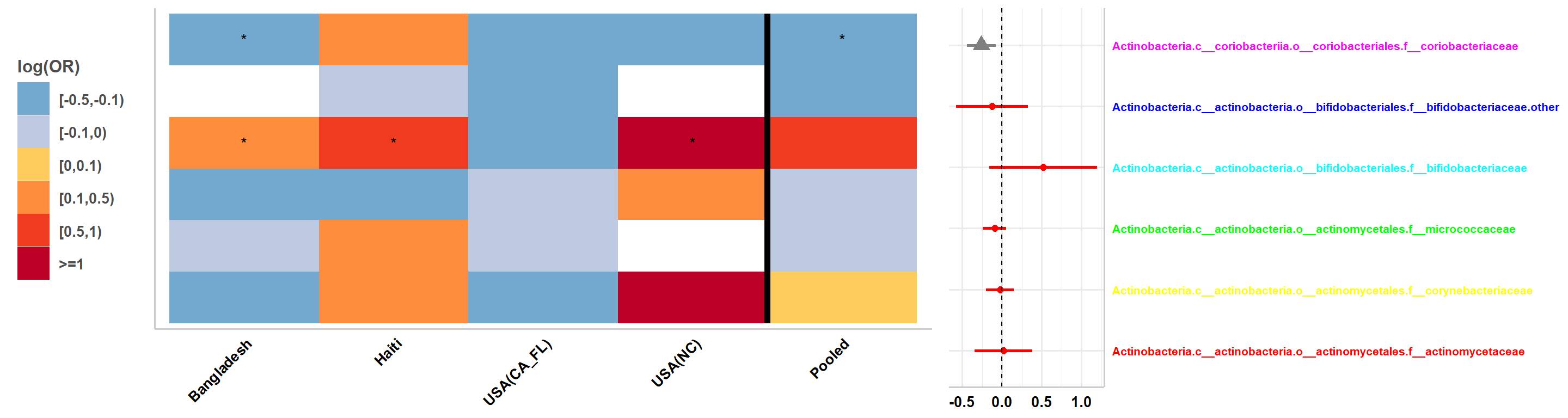
11.5.2.2 Analysis and meta-analysis of other data
Meta-analysis may also be applied for other data such as alpha diversity indexes. For each study, the alpha.compare function imports the outputs from alpha_rarefaction.py QIIME1 script and calculates mean alpha diversity for different indices for each sample based on a user defined rarefaction depth. Mean alpha diversity indexes are standardized to have a mean of 0 and standard deviation of 1 to make these measures comparable across studies. Standardized alpha diversity indexes are compared between groups adjusting for covariates using Linear model for cross sectional data and linear mixed effect model for longitudinal data. Meta-analysis across studies is then done and the results are displayed as a standard meta-analysis forest plot. The example below calculates mean alpha diversity indexes for a selected rarefaction depth, standardizes and compares standardized alpha diversity indexes between groups (male vs. female infants <=6 months of age) adjusting for covariates (feeding status and infant age at sample collection) using the Bangladesh data (Subramanian et al. 2014).
data(alphadat)
data(covar.rm)
covar.rm$sampleid<-tolower(covar.rm$sampleid)
alphacom<-alpha.compare(datlist=alphadat,depth=3,mapfile=covar.rm, mapsampleid="sampleid",comvar="gender",adjustvar=c("age.sample","bf"), longitudinal="yes",age.limit=6,standardize=TRUE)
alphacom$alphasum[,1:5]
## id Estimate.genderMale Std. Error.genderMale t value.genderMale Pr(>|t|).genderMale
## 1 chao1 -0.0654 0.150 -0.435 0.6635
## 2 observed_species -0.1428 0.136 -1.048 0.2947
## 3 pd_whole_tree -0.1325 0.145 -0.912 0.3619
## 4 shannon -0.4401 0.199 -2.208 0.0272Load save result outputs of the alpha.compare function of the four study, and perform meta-analysis using the meta package:
##                  id Estimate.genderMale Std. Error.genderMale t value.genderMale Pr(>|t|).genderMale
## 1             chao1             0.06527                0.0722             0.9042               0.366
## 2  observed_species             0.06529                0.0621             1.0510               0.293
## 3     pd_whole_tree             0.03132                0.0502             0.6233               0.533
## 4           shannon            -0.00128                0.0821            -0.0155               0.988
## 5             chao1            -0.08862                0.3528            -0.2512               0.803
## 6  observed_species            -0.09147                0.3453            -0.2649               0.792
## 7     pd_whole_tree             0.04257                0.2952             0.1442               0.886
## 8           shannon            -0.00911                0.2936            -0.0310               0.975
## 9             chao1            -0.04503                0.1337            -0.3368               0.736
## 10 observed_species            -0.06538                0.1145            -0.5710               0.568
## 11    pd_whole_tree            -0.15902                0.1076            -1.4780               0.139
## 12          shannon            -0.07053                0.1434            -0.4920               0.623
## 13            chao1             0.49658                0.5925             0.8381               0.402
## 14 observed_species             0.23367                0.5294             0.4414               0.659
## 15    pd_whole_tree            -0.01076                0.7331            -0.0147               0.988
## 16          shannon             0.17831                0.5553             0.3211               0.748
##           pop
## 1  Bangladesh
## 2  Bangladesh
## 3  Bangladesh
## 4  Bangladesh
## 5       Haiti
## 6       Haiti
## 7       Haiti
## 8       Haiti
## 9  USA(CA_FL)
## 10 USA(CA_FL)
## 11 USA(CA_FL)
## 12 USA(CA_FL)
## 13   USA(UNC)
## 14   USA(UNC)
## 15   USA(UNC)
## 16   USA(UNC)
# metaanalysis for Shannon index
shannon.sex <- meta::metagen(Estimate.genderMale, `Std. Error.genderMale`, studlab=pop,data=subset(asum4,id=="shannon"),sm="RD", backtransf=FALSE)
meta::forest(shannon.sex,smlab="Standardized \n diversity difference",sortvar=subset(asum4,id=="shannon")$pop,lwd=2)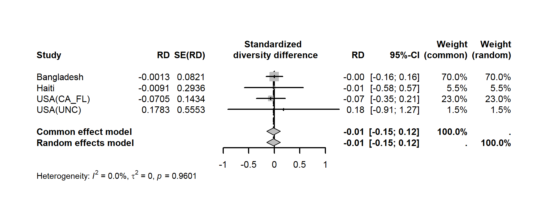
## Number of studies: k = 4
##
##                           RD            95%-CI     z p-value
## Common effect model  -0.0149 [-0.1495; 0.1198] -0.22  0.8288
## Random effects model -0.0149 [-0.1495; 0.1198] -0.22  0.8288
##
## Quantifying heterogeneity (with 95%-CIs):
##  tau^2 = 0 [0.0000; 0.0134]; tau = 0 [0.0000; 0.1157]
##  I^2 = 0.0% [0.0%; 84.7%]; H = 1.00 [1.00; 2.56]
##
## Test of heterogeneity:
##     Q d.f. p-value
##  0.30    3  0.9601
##
## Details of meta-analysis methods:
## - Inverse variance method
## - Restricted maximum-likelihood estimator for tau^2
## - Q-Profile method for confidence interval of tau^2 and tau
## - Calculation of I^2 based on Q## study pval
## [1,] "Bangladesh" "0.987599902164408"
## [2,] "Haiti" "0.9752390484969"
## [3,] "USA(CA_FL)" "0.622739246734807"
## [4,] "USA(UNC)" "0.748126030769876"11.6 Reference materials
- The paper describing the metamicrobiomeR package on BMC Bioinformatics.
- The metamicrobiomeR package hosted in R cran
- An earlier version of the metamicrobiomeR package with full package tutorial on Github