4.1 Main content
- Data types in R: 1D, 2D, special data types
- Subsetting
- Control flow: choices, loops
- Functions
- Errors and error handling in practice
- Coding styles
- How to write a package
Tien Thuy Bui, Msc
Edited by: Nhan Thi Ho, MD, PhD
| Dimension | Homogeneous | Heterogenuous |
|---|---|---|
| 1D | Atomic vector | List |
| 2D | Matrix | Data frame, Tibble |
| n-D | Array |
c(), short for combine:dbl_var <- c(1, 2.5, 4.5)
# With the L suffix, we get an integer rather than a double
int_var <- c(1L, 6L, 10L)
# Use TRUE and FALSE (or T and F) to create logical vectors
log_var <- c(TRUE, FALSE, T, F)
chr_var <- c("these are", "some strings")## [1] 1 2 3 4## [1] 1 2 3 4Given a vector, we can determine its type with typeof(), or check if it’s a specific type with an “is” function: is.character(), is.double(), is.integer(), is.logical(), or, more generally, is.atomic() .
## [1] "double"## [1] TRUE## [1] TRUE## chr [1:2] "a" "1"## [1] 0 0 1## [1] 1## [1] 0.3333333levels of factor defines the set of allowed values.## [1] a b b a
## Levels: a bstringsAsFactors = FALSE## [1] b b a c
## Levels: c < b < a## [,1] [,2] [,3]
## [1,] 1 3 5
## [2,] 2 4 6## [,1] [,2]
## [1,] 1 4
## [2,] 2 5
## [3,] 3 6list() functionnames() function, or directly name inside the list functiontypeof() a list is list. we can test for a list with is.list(), and coerce to a list with as.list() .my_list2 <- list("my_df" = data.frame("col1"=1:5,
"col2"=letters[1:5]),
"my_char"="abc",
"my_num_list" = 1:10 )
my_list2## $my_df
## col1 col2
## 1 1 a
## 2 2 b
## 3 3 c
## 4 4 d
## 5 5 e
##
## $my_char
## [1] "abc"
##
## $my_num_list
## [1] 1 2 3 4 5 6 7 8 9 10## $my_df
## col1 col2
## 1 1 a
## 2 2 b
## 3 3 c
## 4 4 d
## 5 5 e
##
## $my_char
## [1] "abc"
##
## $new_name_for_num_vec
## [1] 1 2 3 4 5 6 7 8 9 10library(tibble)
df1 <- data.frame(x = 1:3, y = letters[1:3]) # y coerced into factor
df2 <- tibble(x = 1:3, y = letters[1:3]) # y not coerced
str(df1)## 'data.frame': 3 obs. of 2 variables:
## $ x: int 1 2 3
## $ y: chr "a" "b" "c"## tibble [3 × 2] (S3: tbl_df/tbl/data.frame)
## $ x: int [1:3] 1 2 3
## $ y: chr [1:3] "a" "b" "c"## [1] "X1"## [1] "1"## x y
## 1 1 1
## 2 2 2
## 3 3 1
## 4 4 2## # A tibble: 4 × 2
## x y
## <int> <dbl>
## 1 1 1
## 2 2 1
## 3 3 1
## 4 4 1## Error in `tibble()`:
## ! Tibble columns must have compatible sizes.
## • Size 4: Existing data.
## • Size 2: Column `y`.
## ℹ Only values of size one are recycled.## # A tibble: 3 × 2
## x y
## <int> <dbl>
## 1 1 2
## 2 2 4
## 3 3 6[[, [, and $.## [1] 2.1 3.3 NA## [1] 4.2 5.4TRUE. This is probably the most useful type of subsetting because we write the expression that creates the logical vector:x <- c(2.1, 4.2, 3.3, 5.4)
# exclude element 2 and 4. Notice how the recycling rule is applied.
x[c(TRUE, FALSE)]## [1] 2.1 3.3## [1] 4.2 3.3 5.4## [1] FALSE TRUE TRUE TRUE## a c
## 2.1 3.3$ is invalid for atomic vector.[ always returns a list; [[ and $ let we pull out elements of a list. $ must be followed by name of a single element.## $a
## [1] 1 2 3 4 5
##
## $b
## [1] "c" "d" "e" "f" "g"
##
## $c
## [1] "I" "J" "K" "L" "M" "N" "O"## [1] 1 2 3 4 5## [1] 1 2 3 4 5## [1] 1 2 3 4 5## $a
## [1] 1 2 3 4 5
##
## $c
## [1] "I" "J" "K" "L" "M" "N" "O"## A B C
## [1,] 1 4 7
## [2,] 2 5 8
## [3,] 3 6 9## A B C
## [1,] 1 4 7
## [2,] 2 5 8# return row #1 and #3 of column B and A. Notice how recylcing rule applies here.
a[c(TRUE, FALSE), c("B", "A")]## B A
## [1,] 4 1
## [2,] 6 3## A C## [,1] [,2] [,3] [,4] [,5]
## [1,] "1,1" "1,2" "1,3" "1,4" "1,5"
## [2,] "2,1" "2,2" "2,3" "2,4" "2,5"
## [3,] "3,1" "3,2" "3,3" "3,4" "3,5"
## [4,] "4,1" "4,2" "4,3" "4,4" "4,5"
## [5,] "5,1" "5,2" "5,3" "5,4" "5,5"## [1] "4,1" "5,3"## x y z
## 1 1 3 a
## 2 2 2 b
## 3 3 1 c## x y z
## 2 2 2 b## x y z
## 1 1 3 a
## 3 3 1 c## x z
## 1 1 a
## 2 2 b
## 3 3 c## x z
## 1 1 a
## 2 2 b
## 3 3 c$ operator also returns a vector## 'data.frame': 3 obs. of 1 variable:
## $ x: int 1 2 3## int [1:3] 1 2 3## int [1:3] 1 2 3if statements and switch() calls, allow us to run different code depending on the input. - Loops, like for and while, allow us to repeatedly run code, typically with changing options.The basic syntax of an if statement in R:
if (condition) { true_action }
if (condition) { true_action } else { false_action }TRUE or FALSE( ){ }x = 56.1
if (x > 90) {
print("A")
} else if (x > 80) {
print("B")
} else if (x > 50) {
print("C")
} else {
print("F")
}## [1] "C"Closely related to if is the switch()-statement. It’s a compact, special purpose equivalent that lets we replace code like:
x = "a"
if (x == "a") {
  "option 1"
} else if (x == "b") {
  "option 2"
} else if (x == "c") {
  "option 3"
} else {
  stop("Invalid `x` value")
}
## [1] "option 1"with the more succinct:
## [1] "option 1"It is recommended to use switch() only with character inputs.
for loops are used to iterate over items in a vector. They have the following basic form: (Notice the use of () - wraps around the sequence and {} - wrap around loop body )for (item in vector) {
perform_action
}set.seed(10)
my_df <- data.frame(a = rnorm(10),
b = rnorm(10),
c = rnorm(10),
d = rnorm(10))
median_vec <- vector("double", ncol(my_df)) # 1. hold-out vector
for (i in seq_along(my_df)) { # 2. sequence
median_vec[i] <- median(my_df[, i]) # 3. body
}
median_vec## [1] -0.3100772 0.6121843 -0.6812107 -0.4880535seq_along() function: generates a sequence the same length of the argument passed. In R, the length of a dataframe is the number of columns.## [1] 1 2 3 4In the case we want to simulate some random vectors of random lengths. we might be tempted to solve this problem by progressively growing the vector (time complexity is O(n^2)).
means <- c(0, 1, 2)
# not efficient
output <- NULL
for (i in seq_along(means)) {
  n <- sample(100, 1)
  output <- c(output, rnorm(n, means[[i]]))
}
str(output)
But this is not very efficient because in each iteration, R has to copy all the data from the previous iterations. This results in O(n^2) complexity! A better solution to initialize a vector or list of fixed length.
## [[1]]
## NULL
##
## [[2]]
## NULL
##
## [[3]]
## NULL
for (i in seq_along(means)) {
n <- sample(100, 1)
out[[i]] <- rnorm(n, means[[i]])
}
str(unlist(out))## num [1:84] -0.0894 0.3148 -2.0605 -0.5998 0.9712 ...We use unlist() to flatten a list of vectors into a single vector.
next exits the current iteration, and move to the next iterationbreak exits the entire for loop.## [1] 3
## [1] 4
## [1] 5for (i in seq_along(xs)), and extracting the value with x[[i]].for (nm in names(xs)). We can use to access the value with xs[[nm]]. This is useful if we want to use the name in a plot title or a file name. If we’re creating named output, make sure to name the results vector like so:results <- vector("list", length(x))
names(results) <- names(x)for (x in xs). This is most useful if we only care about side-effects, like plotting or saving a file, because it’s difficult to save the output efficiently this way.for loops are useful if we know in advance the set of values that we want to iterate over. If we don’t know, there are two related tools with more flexible specifications:
while(condition) action : performs action while condition is TRUE.
repeat(action) : repeats action forever (i.e. until it encounters break).
R does not have an equivalent to the do {action} while (condition) syntax found in other languages.
We can rewrite any for loop to use while instead, and we can rewrite any while loop to use repeat, but the converses are NOT true. That means while is more flexible than for, and repeat is more flexible than while. It’s good practice, however, to use the least-flexible solution to a problem, so we should use for wherever possible.
# Example with while
i = 3
while(i <= 5) {
  print(i)
  i = i + 1 # there should be an increment to update the index. What happend if we dont?
}
## [1] 3
## [1] 4
## [1] 5# Example with repeat
i = 3
repeat {
print(i)
if (i >= 5)
break
i = i + 1 # there should be an increment to update the index. What happend if we dont?
}## [1] 3
## [1] 4
## [1] 5Operates on arrays (including the 2D matrices). General function call:
apply(X, MARGIN, FUN, ...)Where:
- X is an array or a matrix
- MARGIN is a variable defining how the function is applied: when MARGIN=1, it applies over rows, whereas with MARGIN=2, it works over columns. If MARGIN=c(1,2), it applies to both rows and columns; and
- FUN, which is the function that we want to apply to the data.
- Additional arguments to FUN are passed to ...
##            [,1]       [,2]       [,3]       [,4]        [,5]       [,6]
## [1,]  0.2487580  0.6334359  0.4953317 -1.2051854  0.53064987 -0.2498675
## [2,] -1.0626228 -1.9968156  0.7258175 -1.9632525  0.10198345  1.1551047
## [3,] -0.3639822 -0.6818322  0.6672987  1.4707523  1.33778247 -0.8647272
## [4,] -1.2069949 -0.4600555  0.9547864  0.3724723  0.08723477 -0.8666783
## [5,] 1.4292128 -0.9830692 -1.6753322 1.0658793 -0.39110421 -2.3210170## [1] -0.9556291 -3.4883366 1.1679022 -0.2593339 1.6665463 -3.1471854Looping through a vector with apply() will throw an error (why?).
vec <- c(1:10)
apply(vec, 1, sum)
# Error in apply(vec, 1, sum) : dim(X) must have a positive length
*apply(X, FUN, ...)lapply() applies a given function to every element of an object such as list/vector/dataframe/…, and results in a list which has the same number of elements as the object passed to it.X is, the output of lapply() is always a list. To suppess this, feed simplify = TRUE into argument (default value is FALSE).sapply works the same way, but it tries to simplify the output (usually it returns a vector for 1 dimension output or array for higher dimension).# Create a list of matrices
A <- matrix(1:9, ncol = 3)
B <- matrix(1:16, ncol = 4)
C <- cbind(8:10, 8:10)
my_list <- list(A=A, B=B, C=C) # this is a named list
my_list## $A
## [,1] [,2] [,3]
## [1,] 1 4 7
## [2,] 2 5 8
## [3,] 3 6 9
##
## $B
## [,1] [,2] [,3] [,4]
## [1,] 1 5 9 13
## [2,] 2 6 10 14
## [3,] 3 7 11 15
## [4,] 4 8 12 16
##
## $C
## [,1] [,2]
## [1,] 8 8
## [2,] 9 9
## [3,] 10 10# Extract the 2nd column from `my_list` with the selection operator `[` with `lapply()`
# Notice how we pass 2 arguments into the subset operator
lapply(X = my_list, FUN = "[", , 2)## $A
## [1] 4 5 6
##
## $B
## [1] 5 6 7 8
##
## $C
## [1] 8 9 10# Extract the first 2 rows of the 2nd column from `my_list` with the selection operator `[` with `lapply()`
sapply(X = my_list, FUN = "[", 1:2, 2)## A B C
## [1,] 4 5 8
## [2,] 5 6 9mapply(X, FUN, MoreArgs, ...)# times and x are arguments of function rep. Here we apply the rep() functions to 4 values: 1,2,3,4
mapply(x = 1:4, FUN = rep, times = 4)## [,1] [,2] [,3] [,4]
## [1,] 1 2 3 4
## [2,] 1 2 3 4
## [3,] 1 2 3 4
## [4,] 1 2 3 4function|Name <- function(arg1, arg2, arg3=user_default_value){
statement1
statement2
}set.seed(1)
oneSampleTTest <- function(input.data, mu0){
n <- length(input.data)
xbar <- mean(input.data)
s <- sd(input.data)
t <- (xbar - mu0)/(s / sqrt(n))
if( t < 0 ){
p.value <- 2 * pt(t, df=n-1)
}else{
p.value <- 2 * (1-pt(t, df=n-1))
}
cat('t =', t, 'and p.value =', p.value, "\n")
return( list("t"= t, "p.value" = p.value) )
}
test_data <- runif(25, min = 0, max = 25) # 25 random numbers between the values 0 and 10
ttest_val1 <- oneSampleTTest(test_data, mu0=2 )## t = 7.672742 and p.value = 6.556742e-08## $t
## [1] 7.672742
##
## $p.value
## [1] 6.556742e-08## Error in oneSampleTTest(test_data): argument "mu0" is missing, with no defaultoneSampleTTest1 <- function(input.data, mu0 = 1){
n <- length(input.data)
xbar <- mean(input.data)
s <- sd(input.data)
t <- (xbar - mu0)/(s / sqrt(n))
if( t < 0 ){
p.value <- 2 * pt(t, df=n-1)
}else{
p.value <- 2 * (1-pt(t, df=n-1))
}
cat('t =', t, 'and p.value =', p.value, "\n")
return( list("t"= t, "p.value" = p.value) )
}
# test_data <- runif(25, min = 0, max = 25) # 25 random numbers between the values 0 and 10
oneSampleTTest1(test_data )## t = 8.352068 and p.value = 1.460246e-08## $t
## [1] 8.352068
##
## $p.value
## [1] 1.460246e-08if test via function missing()oneSampleTTest2 <- function(input.data){
if(missing(mu0) ){
mu0 <- 1
}
n <- length(input.data)
xbar <- mean(input.data)
s <- sd(input.data)
t <- (xbar - mu0)/(s / sqrt(n))
if( t < 0 ){
p.value <- 2 * pt(t, df=n-1)
}else{
p.value <- 2 * (1-pt(t, df=n-1))
}
cat('t =', t, 'and p.value =', p.value, "\n")
return( list("t"= t, "p.value" = p.value) )
}
oneSampleTTest2(test_data )## Error in oneSampleTTest2(test_data): 'missing(mu0)' did not find an argumentdo.call() has two arguments. The function to call, and a list containing the function arguments:
## t = 7.672742 and p.value = 6.556742e-08## $t
## [1] 7.672742
##
## $p.value
## [1] 6.556742e-08Many functions in R take an arbitrary number of inputs:
## [1] 55## [1] "a, b, c, d, e, f, g, h, i, j"# pass ... to another function
printCommas <- function(...){
print(paste("There are", length(...), "elements:", commas(...) ))
}
printCommas(letters[1:10])## [1] "There are 10 elements: a, b, c, d, e, f, g, h, i, j"Functions can be defined inside an *apply() call. For example:
## [1] 1.742187 1.160036 1.927549 1.480127 1.187428Names defined inside a function mask names defined outside a function. This is illustrated in the following example:
## x = 1 y = 2If a name isn’t defined inside a function, R looks one level up.
## x = 2 y = 1What if we call y in global environment?
## [1] 20The same rules apply if a function is defined inside another function. First, R looks inside the current function. Then, it looks where that function was defined (and so on, all the way up to the global environment). Finally, it looks in other loaded packages.
## [1] 1 2 3my_func() yet. This behaviour is called lazy evaluation## [1] 110## [1] 1010codetools::findGlobals(). This function lists all the external dependencies (unbound symbols) within a function:## [1] "{" "+" "y"There are two ways that a function can return a value: implicitly (without a return statement) and explicitly (with a return statement)
For implicit return, the last evaluated expression is the return value.
The same example, with a return statement:
From the previous example, the functions return visibly: calling the function in an interactive context prints the result.
We can prevent automatic printing by applying invisible() to the last value
data(iris)
show_missings <- function(df) {
  n <- sum(is.na(df))
  # cat("Missing values: ", n, "\n", sep = "")
  if( n == 0)
    invisible(df)
  else
    NULL
}
show_missings(iris) # print nothing
To verify that this value does indeed exist, we can explicitly print it or wrap it in parentheses:
##   Sepal.Length Sepal.Width Petal.Length Petal.Width Species
## 1          5.1         3.5          1.4         0.2  setosa
## 2          4.9         3.0          1.4         0.2  setosa
## 3          4.7         3.2          1.3         0.2  setosa
## 4          4.6         3.1          1.5         0.2  setosa
## 5          5.0         3.6          1.4         0.2  setosa
## 6 5.4 3.9 1.7 0.4 setosaErrors most often occur when code is used in a way that it is not intended to be used. For example adding two strings together produces the following error:
## Error in "hello" + "world": non-numeric argument to binary operatoradd <- function(x, y){
if (!is.numeric(x) || !is.numeric(y)) # OR operator
stop("Error! x and y must be numeric")
x + y
}
add(3, 2)## [1] 5## Error in add("hello", "world"): Error! x and y must be numericWarnings, signalled by warning(), are weaker than errors: they signal that something has gone wrong, but the code has been able to recover and continue.
## [1] NaNIn a user defined function:
sqrtExt <- function(x){ # square root of complex number
  if(! is.numeric(x))
    stop("Error! x must be numeric")
  else if (x < 0) {
    warning("x has negative value. Complex number produced! \n")
    x = x + 0i
  }
  return(sqrt(x))
}

sqrtExt(-4)
## [1] 0+2iMessages, signalled by message(), are informational; we generate a message to tell the user that the code has done something on their behalf. Good messages are a balancing act: we want to provide just enough information so the user knows what’s going on, but not so much that they’re overwhelmed.
Remember this histogram sketch from ggplot2?
library(ggplot2)
rnorm_df <- data.frame(x = rnorm(n=100))
ggplot(data = rnorm_df, mapping = aes(x=x)) + geom_histogram()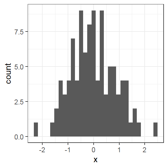
We can provide a message in our own function:
plot_histogram <- function(x, bins, ...){
  if (missing (bins)) # check if argument bins is provided (indicating number of bins)
    message("`plot_histogram()` uses `bins=30` by default. Pick better value with `bins=` ")
    bins = 30
  hist(x, breaks=bins)
}
plot_histogram(rnorm_df$x)
## `plot_histogram()` uses `bins=30` by default. Pick better value with `bins=`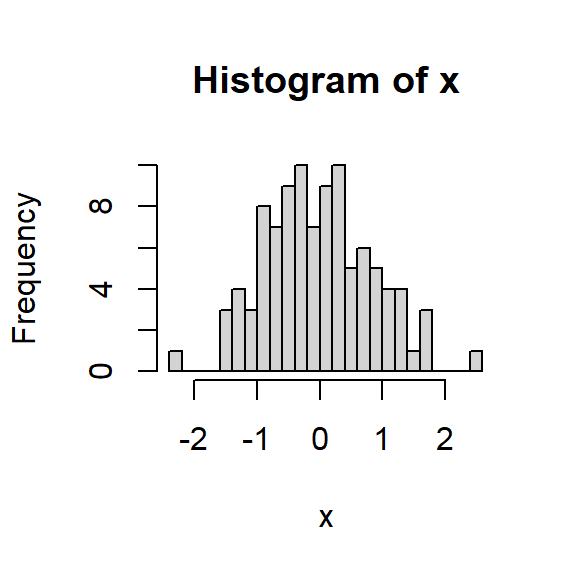
progress) is better, but a message is a good place to start.tryCatch() function is the workhorse of handling errors and warnings in R.try() function is a wrapper function for trycatch() which prints the error and then continues. On the other hand, trycatch() gives us the control of the error function and also optionally, continues the process of the function.Let’s first define a function that takes an expression as an argument and tries to evaluate it.
## [1] 4## [1] 1 NA 3## Error in 2 + "two": non-numeric argument to binary operatorWhat if the beera(2 + "two") evaluation was called the first ? We cannot proceed to the other two lines.
Now let’s use tryCatch() to catch the errors and warnings.
beera <- function(expr){
  tryCatch(expr,
         error = function(e){
           message("An error occurred:", e) # e is the error message generated by R
         },
         warning = function(w){
           message("A warning occured:", w)
         },
         finally = { # this always shows
           message("Finally done!")
         })
}

beera(2 + "two")
beera(2 + 2)
## [1] 4Consider our self defined is_even() function.
## Error in n%%2: non-numeric argument to binary operatorLet’s catch the error, and return some indicating value when an error happens.
is_even <- function(n){
  tryCatch(n %% 2 == 0,
           error = function(e){
             message("An error occurred: ", e, "Returning NA value")
             return(NA)
           })
}

is_even(714)
## [1] TRUE## [1] FALSE## [1] NAprint() lacks the lack of embedded concatenation of terms. We have to relay on paste() for concatenationprint() also prints out quotation mark## [1] "Hello World!"cat() addresses all of these critiques. By default, cat() adds space between terms. To suppress or change this, we can use sep argument.## our x value is 10!message() function is one step further than cat() ! It changed the color from standard black output to red output to catch the users eye. (similar to stop and warning).R is a high-level programming language used primarily for statistical computing and graphics. The goal of the R Programming Style Guide is to make our R code easier to read, share, and verify. There are a few conventions recommended by Google’s R style guide.
<- , not =. Hot key for RStudio is Alt + = keys.. in our object names. It can cause confusion with methods in S3 class in R, and in other object-oriented programming languages.# Good
doNothing <- function() {
return(invisible(NULL))
}
first_name <- "Ngoc"
# not recommended: "." in object name.
first.name <- "Sang"attach() when loading a package. The possibilities for creating errors when using attach() are numerous. library or require are for this purposesuppressPackageStartupMessages(library(dplyr))
# Bad
iris %>%
dplyr::summarize(max_petal = max(Petal.Width)) -> resultsreturn()) makes functions clearer."I wish I'd left this code across scattered .R files instead of combining it into a package" said no one ever #rstats http://t.co/udeNH4T67H
— David Robinson ((drob?)) June 19, 2015
roxygen2 for documenting our functions (see below).myfirstpackage.Rproj: This is a RStudio specific file.R/load_mat.R and add the following contents to the file:#' @export
load_mat <- function(infile){
in.dt <- data.table::fread(infile, header = TRUE)
in.dt <- in.dt[!duplicated(in.dt[, 1]), ]
in.mat <- as.matrix(in.dt[, -1, with = FALSE])
rownames(in.mat) <- unlist(in.dt[, 1, with = FALSE])
in.mat
}@export tag above the functions to make it available for users to use. Otherwise they cannot assess these functions when installing the package in their system#' @export syntax is actually an Roxygen tag. By doing this, this ensures that the load_mat() function gets added to the NAMESPACE (when we run devtools::document()) to indicate that it needs to be exposed.load_mat() function actually depends on the data.table::fread() function to read in files super quickly. NOTICE the double colon “:” used to directly call fread() from data.table packagelibrary() or require() when writing an R packageDESCRIPTION file under the Imports content. For this case, we need the data.table R package, so we added the following to our DESCRIPTION file:# Notice how we also specified the version of the data.table
Imports:
data.table (>= 1.9.4)
dplyrroxygen2 which provides a very simple way of documenting our functions and then produces man/load_mat.Rd files which is what we see when we go ?load_mat.#' Load a Matrix
#'
#' This function loads a file as a matrix. It assumes that the first column
#' contains the rownames and the subsequent columns are the sample identifiers.
#' Any rows with duplicated row names will be dropped with the first one being
#' kepted.
#'
#' @param infile Path to the input file
#' @return A matrix of the infile
#' @export
load_mat <- function(infile){
  in.dt <- data.table::fread(infile, header = TRUE)
  in.dt <- in.dt[!duplicated(in.dt[, 1]), ]
  in.mat <- as.matrix(in.dt[, -1, with = FALSE])
  rownames(in.mat) <- unlist(in.dt[, 1, with = FALSE])
  in.mat
}devtools::document().Rd file for each function in our R package.devtools::document() again to re-generate the .Rd files.load_mat.Rd file is generated in the man folder:% Generated by roxygen2 (4.1.0): do not edit by hand
% Please edit documentation in R/load.R
\name{load_mat}
\alias{load_mat}
\title{Load a Matrix}
\usage{
load_mat(infile)
}
\arguments{
\item{infile}{Path to the input file}
}
\value{
A matrix of the infile
}
\description{
This function loads a file as a matrix. It assumes that the first column
contains the rownames and the subsequent columns are the sample identifiers.
Any rows with duplicated row names will be dropped with the first one being
kepted.
}devtools::use_vignette("introduction")usethis package. So if we are using a newer version of devtools, we can run:usethis::use_vignette("introduction")vignette/introduction.Rmd file. This is a vignette template Rmarkdown file that we can then use to fill out steps on how we can use our package.devtools::install() function which installs our R package into our R system library. Then we will be able to load up our package with:library("myfirstpackage")devtools::install_github("yourusername/myfirstpackage")