Chapter 8 Survival Data Analysis with R

Ho Thi Nhan, MD, PhD

8.1 What is survival analysis?

Survival analysis is the study of survival times and of the factors that influence them.
Survival analysis investigates the time it takes for an event of interest to occur (time-to-event).

8.1.1 Examples of survival analysis

Time from birth until death
Time from entry into a clinical trial until tumor response
Time from treatment initiation to disease recovery

And much more…

8.1.2 Other application of survival analysis

Reliability analysis
Duration analysis
Event history analysis
Time-to-event analysis

8.1.3 Survival data

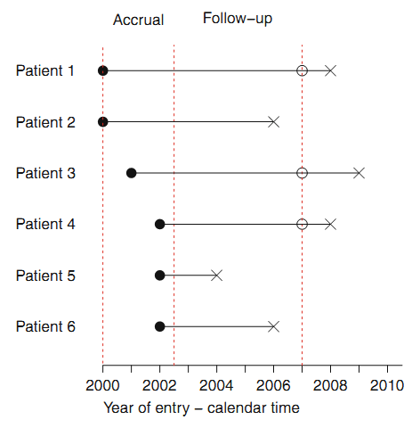
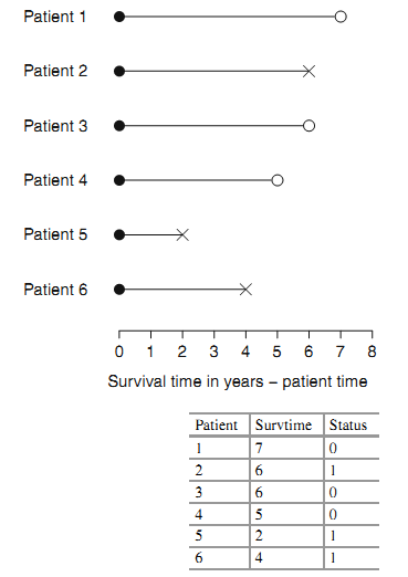
Response variable is a non-negative discrete or continuous random variable, and represents the time from a well-defined origin to a well-defined event (distinct start time and end time).
Survival data is often represented as a pair ( $t_{i}$ ; $\delta_{i}$ ) where t is the time until endpoint or last follow-up, and $\delta$ is a 0/1 variable with 0= “subject was censored at t” and 1 = “subject had an event at t”, or in R code as Surv(time, status).

8.1.3.1 Censoring

Starting or ending events are not precisely observed
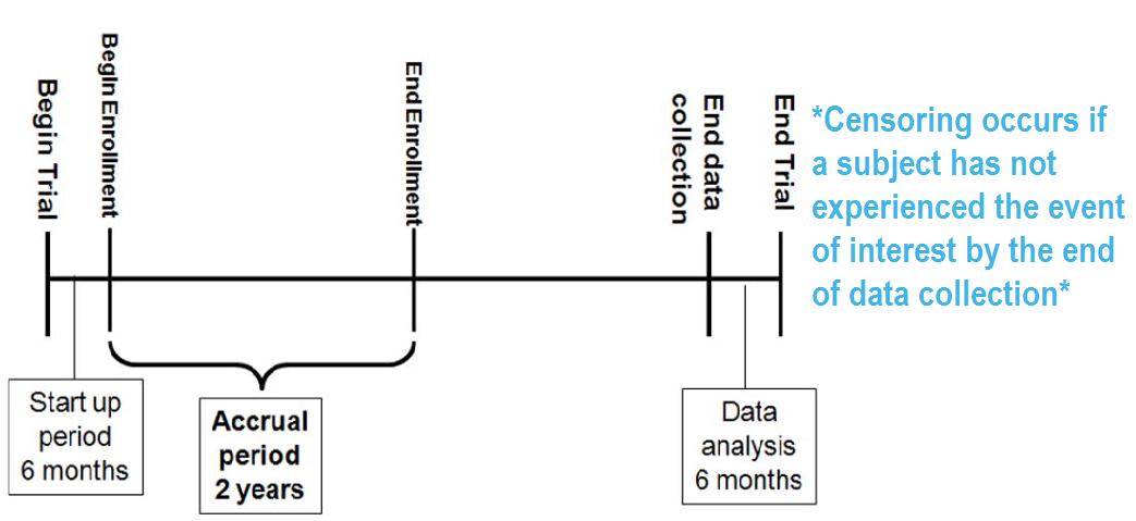
Right censoring (most common): At the time of an analysis, not everyone will have yet had the event. The final endpoint is only known to exceed a particular value $\rightarrow$ Incomplete/partial information: if a particular subject was enrolled in a study 2 years ago, and has not yet had an event at the time of analysis, we only know that their time to event is > 2 years.

Right censoring: trial example:

Source: Survival Analysis in R

8.1.3.2 Types of censoring

8.1.3.2.1 Three types of censoring:

Type I: censoring times are pre-specified. E.g. cohort of patients may start at a specific time, and all followed until a pre-specified ending time. Patients who have not experienced the event of interest before the end of the study are then censored at that time.
Type II: experimental objects are followed until a prespecified fraction have failed. Such a design is rare in biomedical studies, but may be used in industrial settings, where time to failure of a device is of primary interest. E.g. the study stops after 40 out of 100 devices are observed to fail. The remaining 60 devices would then be censored. In this example, the smallest 40% of the ordered failure times are observed, and the remainder are censored.
Random: Careful attention to the cause of the censoring is essential in order to avoid biased survival estimates.

8.1.3.2.2 Examples of random censoring

Participant drop-out: If the dropout occurs truly at random, and is unrelated to the disease process, such censoring may not cause any problems with bias in the analysis. But if patients who are near death are more likely to drop out than other patients, serious biases may arise.
Competing risk (e.g. died of another cause before died of the cause of interest).
Most common source of random censoring is administrative censoring, which results because some patients in a clinical trial have not yet died at the time the analysis is carried out.

8.1.3.3 Survival data: Clinical trial example

Example clinical trial accrual and follow-up periods:

The vertical dashed lines indicate the trial start, end of accrual, and end of follow-up time. The Xs denote death and the open circles denotes censoring events.

8.1.3.4 Compute time-to-event data

Example survival data, patient time:

8.1.3.5 Distribution of time-to-event data

Always positive.
Skewed, may differ between censored patients and those with events.

Example distribution of time-to-event data:

8.1.4 Survival models

8.1.4.1 For multiple event models

Example multiple event models:

Source: A package for survival analysis in R.

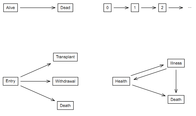
8.1.4.2 2 by 2 division of survival data sets

One event per subject	Multiple events per subject
One event type	1	2
Multiple event type	3	4

1: “Classic” simple survival with two states of alive and dead (upper left) $\rightarrow$ main topic of this module.
2: Repeated events of the same type (upper right).
3: Competing risk (lower left).
4: Illness-death model (lower right).

8.2 Some math definitions

8.2.1 The Hazard and Survival Functions

The survival function defines the probability of surviving up to a point t: $S(t)=pr(T>t), 0<t<Inf$ .
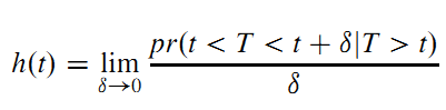
The hazard function is the instantaneous failure rate: the probability that, given that a subject has survived up to time t, he or she fails in the next small interval of time, divided by the length of that interval (Moore 2016):

8.2.2 Other Representations of a Survival Distribution

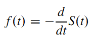
The probability density function (PDF) is minus the rate of change of the survival function:

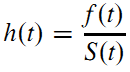
The hazard at time t is the probability that an event occurs in the neighborhood of time t divided by the probability that the subject is alive at time t. The hazard function is related to the PDF and survival functions by:

The cumulative hazard function is defined as the area under the hazard function up to time t:

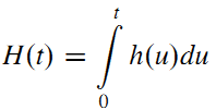
The survival function may be defined in terms of the hazard function by:

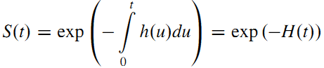
$\rightarrow$ May compute the survival function corresponding to a hazard function.

8.3 Working with survival data in R

8.3.1 R packages for survival data analysis

CRAN Task View: Survival Analysis.

8.3.2 Three main packages

Essential core package: “survival” (Therneau 2024).
Package for nice visualization and more: “survminer” (Kassambara, Kosinski, and Biecek 2024)
Package for working with dates (to create time to event data): “lubridate” (Spinu, Grolemund, and Wickham 2024)

#install.packages(c("survival","survminer","lubridate"))
#load multiple packages
lapply(c("survival","survminer","lubridate","rio","tidyverse","knitr"), library, character.only = TRUE)

8.3.3 Working with dates

Data will often come with start and end dates rather than pre-calculated survival times.

Make sure these dates are formatted as dates in R.
Calculate survival time (time-to-event)

exdate<-read.table("https://stats.idre.ucla.edu/stat/r/examples/asa/hmohiv.csv", sep=",", header = TRUE)
#dates with base R
# calculate the number of days between our two dates and convert it to a numeric value using as.numeric. Then convert to month by dividing by 30.42. 
exdateb<-exdate %>%
  mutate_at(c("entdate","enddate"), as.Date, format="%m/%d/%Y")%>%
  mutate(
    ttevent.m=as.numeric(
      difftime(enddate,
             entdate,
             units="days"))/30.42)
head(exdateb)

#with lubridate
exdatel<-exdate%>%
  mutate_at(c("entdate","enddate"), mdy)%>%
  mutate(
    ttevent.m=interval(entdate,enddate)/months(1))
head(exdatel)

#rename
exdatel<-exdatel%>%
  rename(status=censor)

8.3.4 Package “survival” main functions

8.3.4.1 Surv()

Surv(time, status): right censored data
Surv(time, endpoint==‘death’): right censored data, where the status variable is a character or factor
Surv(t1, t2, status): counting process data
Surv(t1, ind, type=‘left’): left censoring
Surv(time, fstat): multiple state data, fstat is a factor

8.3.4.2 coxph() Cox’s proportional hazards model.

coxph(Surv(time, status) ~ x, data=aml) : standard Cox model
coxph(Surv(t1, t2, stat) ~ (age + surgery)* transplant): time dependent covariates.
y <- Surv(t1, t2, stat) coxph(y~strata(inst) * sex + age + treat): Stratified model, with a sepa- rate baseline per institution, and institution specific effects for sex.
coxph(y ~ offset(x1) + x2) : force in a known term, without estimating a coeffcient for it.

8.3.4.3 cox.zph

Computes a test of proportional hazards for the fitted Cox model.

zfit <- cox.zph(coxfit); plot(zfit).

8.3.4.4 survreg

Parametric survival models.

survreg(Surv(time, stat) ~x, dist=“loglogistic”) : Fit a log-logistic distribution.

8.3.4.5 survfit Fit a survival curve.

survfit(Surv(time, status)): Simple Kaplan-Meier
survfit(Surv(time, status) ~ rx + sex) : Four groups
fit <- coxph(Surv(time, stat) ~ rx + sex) survfit(fit, list(rx=1, sex=2)): Predict curv

8.3.4.6 survdiff testing difference between survival curves

One and k-sample versions of the Fleming-Harrington G family. Includes the logrank and Gehan-Wilcoxon as special cases.

survdiff(Surv(time, status) ~ sex + treat) : Compare the 4 sub-groups formed by sex and treatment combinations.
survdiff(Surv(time, status) ~ offset(pred)): One-sample test

8.3.5 Survival curves and models

8.3.5.1 Survival model and curve for overall data

fit1 <- survfit(Surv(time, status) ~ 1, data=lung)
print(fit1)

## Call: survfit(formula = Surv(time, status) ~ 1, data = lung)
## 
##        n events median 0.95LCL 0.95UCL
## [1,] 228    165    310     285     363

#summary(fit1)

Median survival time

lung %>% filter(status==1)%>%
  summarise(med_surv=median(time))

##   med_surv
## 1      284

Right or wrong? Why?

$\rightarrow$ Wrong as censoring is ignored.

The correct estimate is:

print(fit1)

## Call: survfit(formula = Surv(time, status) ~ 1, data = lung)
## 
##        n events median 0.95LCL 0.95UCL
## [1,] 228    165    310     285     363

Survival as specific time point, for example survival at 1 year:

evy1<-lung %>% 
  filter(time<=365 & status==1) %>%
  summarise(
    sum(as.numeric(as.character(status)))) 
1-evy1/nrow(lung)

##   sum(as.numeric(as.character(status)))
## 1                             0.8157895

Right or wrong? Why?

$\rightarrow$ Wrong as censoring is ignored.

The correct estimate for 1 year survival is:

summary(fit1, times = 365)

## Call: survfit(formula = Surv(time, status) ~ 1, data = lung)
## 
##  time n.risk n.event survival std.err lower 95% CI upper 95% CI
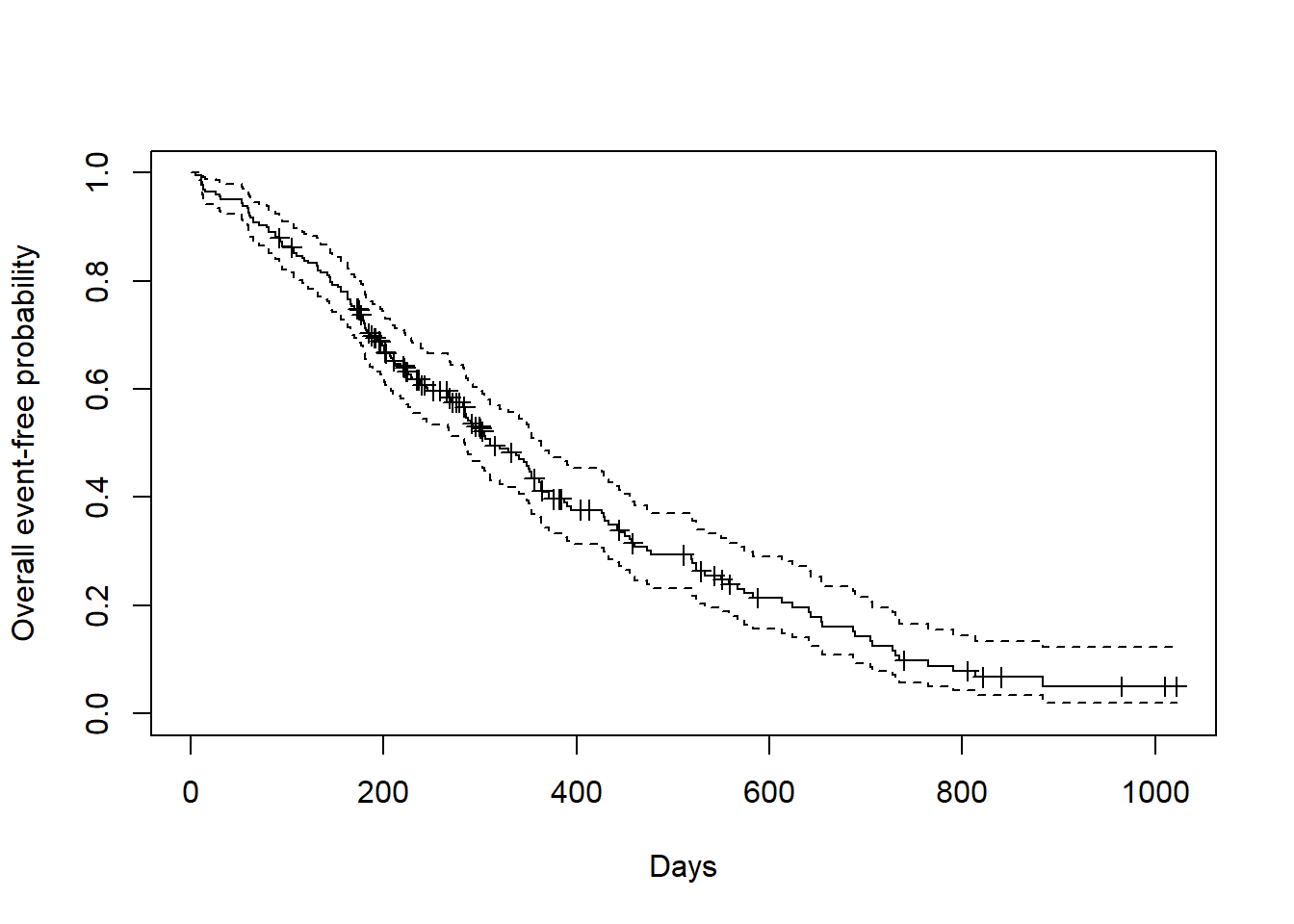
##   365     65     121    0.409  0.0358        0.345        0.486

Kaplan-Meier plot using base R

plot(fit1, mark.time = TRUE,
     xlab = "Days", 
     ylab = "Overall event-free probability")

Kaplan-Meier plot using survminer package.

ggsurvplot(
  fit=fit1,
  risk.table = TRUE,
  risk.table.height = 0.3,
  xlab = "Days", 
  ylab = "Overall event-free probability")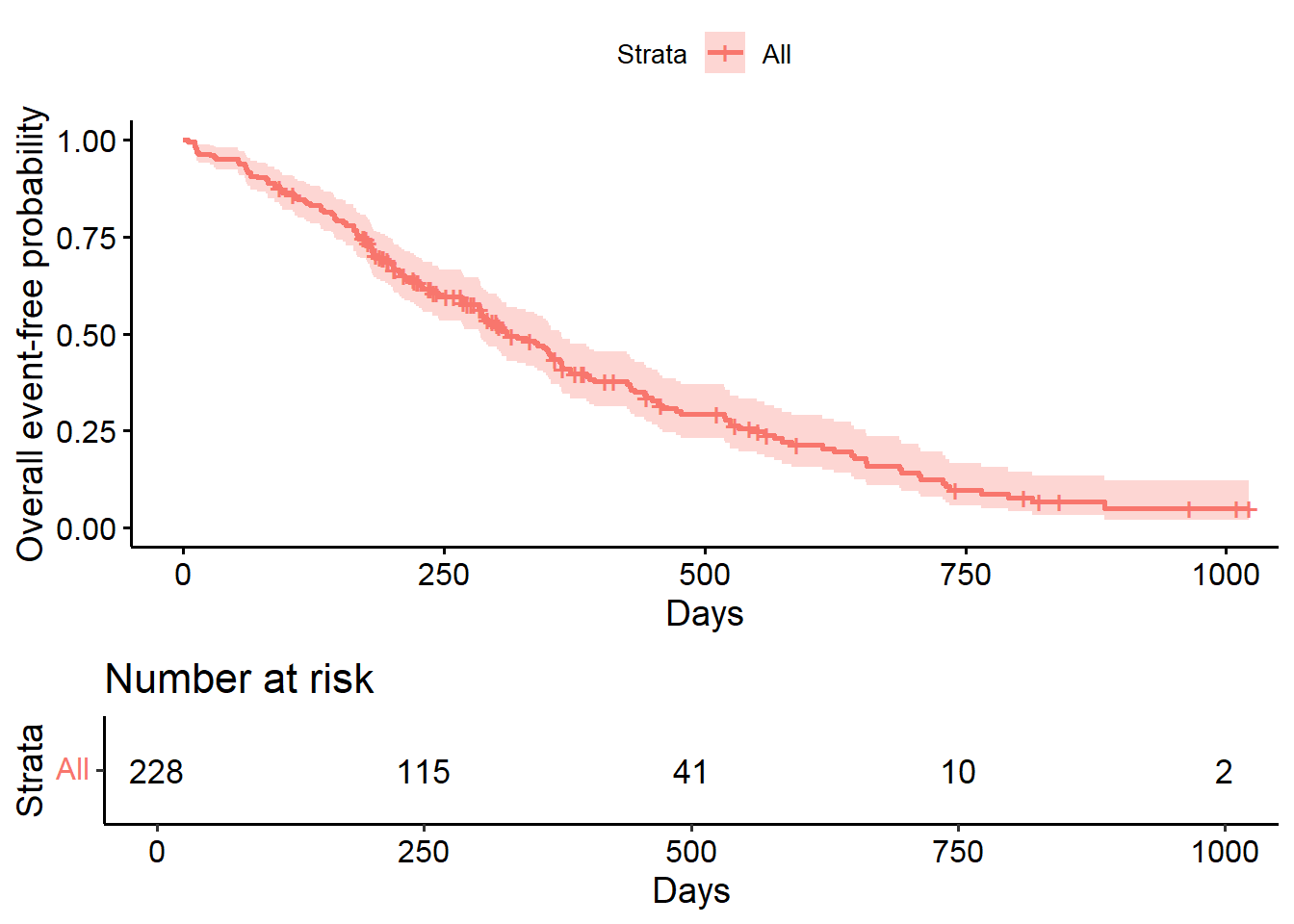

8.3.5.2 Comparing survival times between groups

fit2 <- survfit(Surv(time, status) ~ sex, data=lung)
print(fit2)

## Call: survfit(formula = Surv(time, status) ~ sex, data = lung)
## 
##         n events median 0.95LCL 0.95UCL
## sex=1 138    112    270     212     310
## sex=2  90     53    426     348     550

#summary(fit2)

8.3.5.2.1 Testing the difference

The most common way to compare survival times between groups is log-rank test (or Mantel-Haenszel test) which equally weights observations over the entire follow-up time. (rho=0 for log rank test (default); rho=1 for Peto-Wilcoxon test).

The log-rank test is equivalent to the score test from a Cox model with the group as a factor variable.

survdiff(Surv(time, status) ~ sex,data=lung)

## Call:
## survdiff(formula = Surv(time, status) ~ sex, data = lung)
## 
##         N Observed Expected (O-E)^2/E (O-E)^2/V
## sex=1 138      112     91.6      4.55      10.3
## sex=2  90       53     73.4      5.68      10.3
## 
##  Chisq= 10.3  on 1 degrees of freedom, p= 0.001

survdiff(Surv(time, status) ~ sex,rho=1, data=lung)

## Call:
## survdiff(formula = Surv(time, status) ~ sex, data = lung, rho = 1)
## 
##         N Observed Expected (O-E)^2/E (O-E)^2/V
## sex=1 138     70.4     55.6      3.95      12.7
## sex=2  90     28.7     43.5      5.04      12.7
## 
##  Chisq= 12.7  on 1 degrees of freedom, p= 4e-04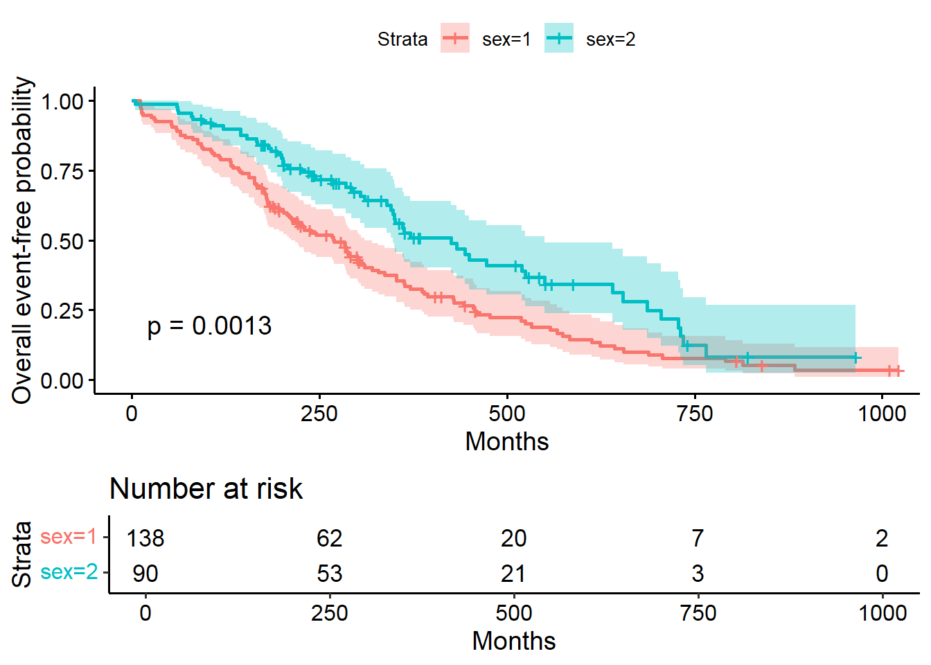

8.3.5.2.2 KM between groups with survminer

ggsurvplot(
  fit=fit2,
  conf.int = TRUE,
  pval = TRUE, 
  risk.table = TRUE,
  risk.table.height = 0.3,
  xlab = "Months", 
  ylab = "Overall event-free probability")

8.3.5.3 The Cox regression model

Semi-parametric model to fit univariable and multivariable regression models for survival outcomes.
Some key assumptions of the model: non-informative censoring and proportional hazards.
Most commonly used for single event data (one event per subject)
Proportional hazards models differ from other types of regression: there is no intercept term (intercept term, if any, absorbed into the baseline hazard).
$\psi$ indexes the difference between the two survival distributions via the Lehmann alternative: $S_{1}(t)=[S_{0}(t)]^{\psi}$ . This relationship can be re-expressed in terms of the hazard functions, yielding proportional hazards assumption: $h_{1}(t)=\psi h_{0}(t)$ .
The model can be extended to include covariate information in a vector z as follows: $\psi=e^{z\beta}$ (Moore 2016).

cfit1 <- coxph(Surv(time, status) ~ sex,data=lung)
print(cfit1, digits=3)

## Call:
## coxph(formula = Surv(time, status) ~ sex, data = lung)
## 
##       coef exp(coef) se(coef)     z      p
## sex -0.531     0.588    0.167 -3.18 0.0015
## 
## Likelihood ratio test=10.6  on 1 df, p=0.00111
## n= 228, number of events= 165

#print routine gives a short summary and the summary routine a longer one
summary(cfit1, digits=3)

## Call:
## coxph(formula = Surv(time, status) ~ sex, data = lung)
## 
##   n= 228, number of events= 165 
## 
##        coef exp(coef) se(coef)      z Pr(>|z|)   
## sex -0.5310    0.5880   0.1672 -3.176  0.00149 **
## ---
## Signif. codes:  0 '***' 0.001 '**' 0.01 '*' 0.05 '.' 0.1 ' ' 1
## 
##     exp(coef) exp(-coef) lower .95 upper .95
## sex     0.588      1.701    0.4237     0.816
## 
## Concordance= 0.579  (se = 0.021 )
## Likelihood ratio test= 10.63  on 1 df,   p=0.001
## Wald test            = 10.09  on 1 df,   p=0.001
## Score (logrank) test = 10.33  on 1 df,   p=0.001

#likelihood ratio test
anova(cfit1)

## Analysis of Deviance Table
##  Cox model: response is Surv(time, status)
## Terms added sequentially (first to last)
## 
##       loglik  Chisq Df Pr(>|Chi|)   
## NULL -749.91                        
## sex  -744.59 10.634  1   0.001111 **
## ---
## Signif. codes:  0 '***' 0.001 '**' 0.01 '*' 0.05 '.' 0.1 ' ' 1

cfit0 <- coxph(Surv(time, status) ~ 1,data=lung)
anova(cfit1,cfit0)

## Analysis of Deviance Table
##  Cox model: response is  Surv(time, status)
##  Model 1: ~ sex
##  Model 2: ~ 1
##    loglik  Chisq Df Pr(>|Chi|)   
## 1 -744.59                        
## 2 -749.91 10.634  1   0.001111 **
## ---
## Signif. codes:  0 '***' 0.001 '**' 0.01 '*' 0.05 '.' 0.1 ' ' 1

8.3.5.3.1 Hazard ratios

HR represents the ratio of hazards between two groups at any particular point in time.
Interpreted as the instantaneous rate of occurrence of the event of interest in those who are still at risk for the event. It is not a risk, though it is commonly interpreted as such
$HR = exp(\beta)$ (exponentiation of coefficients of Cox model output)
A HR < 1 indicates reduced hazard of event whereas a HR > 1 indicates an increased hazard of event. So our HR = 2.28 (drug) implies that around 2.28 times as many of those using drug are having the event as compared to those not using drug, at any given time.

8.3.5.3.2 Multivariate Cox model

# covariates
cfit2 <- coxph(Surv(time, status) ~ sex+age,data=lung)
print(cfit2, digits=3)

## Call:
## coxph(formula = Surv(time, status) ~ sex + age, data = lung)
## 
##         coef exp(coef) se(coef)     z      p
## sex -0.51322   0.59857  0.16746 -3.06 0.0022
## age  0.01705   1.01719  0.00922  1.85 0.0646
## 
## Likelihood ratio test=14.1  on 2 df, p=0.000857
## n= 228, number of events= 165

summary(cfit2, digits=3)

## Call:
## coxph(formula = Surv(time, status) ~ sex + age, data = lung)
## 
##   n= 228, number of events= 165 
## 
##          coef exp(coef)  se(coef)      z Pr(>|z|)   
## sex -0.513219  0.598566  0.167458 -3.065  0.00218 **
## age  0.017045  1.017191  0.009223  1.848  0.06459 . 
## ---
## Signif. codes:  0 '***' 0.001 '**' 0.01 '*' 0.05 '.' 0.1 ' ' 1
## 
##     exp(coef) exp(-coef) lower .95 upper .95
## sex    0.5986     1.6707    0.4311    0.8311
## age    1.0172     0.9831    0.9990    1.0357
## 
## Concordance= 0.603  (se = 0.025 )
## Likelihood ratio test= 14.12  on 2 df,   p=9e-04
## Wald test            = 13.47  on 2 df,   p=0.001
## Score (logrank) test = 13.72  on 2 df,   p=0.001

8.3.5.3.3 Stratified Cox model

Adding one or more strata terms to the model formula.
Each subject is compared only to subjects within their own stratum for computing the partial likelihood, and then the final results are summed over the strata.
Variable included as a stratum is adjusted for in the most general way, and not having an estimate of its effect.
Common use of strata: to adjust for the enrolling institution in a multi-center study.

# Example 
cfit <- coxph(Surv(time, status) ~ age + sex + wt.loss, data=lung)
#summary(cfit)
cfits <- coxph(Surv(time, status) ~ age + sex + wt.loss + strata(inst),
data=lung)
#summary(cfits)
# compare between simple and stratified models
round(cbind(simple= coef(cfit), stratified=coef(cfits)), 4)

##          simple stratified
## age      0.0201     0.0235
## sex     -0.5210    -0.5160
## wt.loss  0.0008    -0.0017

8.3.6 Model selection & Interpretation

8.3.6.1 Partial Likelihood Hypothesis Tests

Three forms of test for H0: $\beta$ = 0:

Wald test: commonly used test, from output: Z= $\hat{\beta}$ /s.e.( $\hat{\beta}$ )
Score test: equivalent to the log-rank test
Likelihood ratio test: key advantage of this test over the other two is that it is invariant to monotonic transformations of $\beta$ .

8.3.6.2 Hypothesis Testing for Nested Models

Survival Model: log( $\psi$ )= $z_{1i}$ $\beta_{1}$ + $z_{2i}$ $\beta_{2}$ +…+ $z_{ki}$ $\beta_{k}$ . Where $\beta_{k}$ is the log hazard ratio.

#anova command shows likelihood ratio tests for each term in a model, added sequentially
anova(cfit)

## Analysis of Deviance Table
##  Cox model: response is Surv(time, status)
## Terms added sequentially (first to last)
## 
##          loglik  Chisq Df Pr(>|Chi|)   
## NULL    -680.39                        
## age     -677.78 5.2273  1   0.022235 * 
## sex     -673.06 9.4268  1   0.002138 **
## wt.loss -673.06 0.0150  1   0.902592   
## ---
## Signif. codes:  0 '***' 0.001 '**' 0.01 '*' 0.05 '.' 0.1 ' ' 1

8.3.6.3 Model selection approaches

Large number of potential factors $\rightarrow$ need to prune the model so that only necessary covariates are included.

Step-wise:

Forward: univariate model for each covariate $\rightarrow$ choose ones with smallest p-values to fit models with two covariates $\rightarrow$ common critical p-values are 5% and 10%.
Backward: fit all variables $\rightarrow$ remove one by one with largest p-value
Problems: 1) multiple comparisons: p-values from one stage to another are not the same; 2) P-values only valid for nested models.

8.3.6.4 The Akaike Information Criterion (AIC) for Comparing Non-nested Models

AIC= $-2*l(\hat{\beta})+2*k$ , where:

$-2*l(\hat{\beta})$ is goodness of fit (smaller the better), denotes the value of the partial log likelihood at the M.P.L.E. for a particular model.
k is the number of parameters in the model = measure of complexity.

AIC(cfit)

## [1] 1352.112

AIC(cfits)

## [1] 577.052

# Using AIC for "step" model selection
#fitall<-coxph(Surv(time, status) ~ age + sex + wt.loss+ inst+ ph.ecog+ ph.karno+ meal.cal, data=lung)
#anova(fitall)
#aicstep<-step(fitall, scope=list(upper=~age +sex + wt.loss+ inst+ ph.ecog+ ph.karno+ meal.cal, lower=~age))
lung.nona<-na.omit(lung)
fitall2<-coxph(Surv(time, status) ~ age + sex + wt.loss+ inst+ ph.ecog+ ph.karno+ meal.cal, data=lung.nona)
aicstep2<-step(fitall2, scope=list(upper=~age +sex + wt.loss+ inst+ ph.ecog+ ph.karno+ meal.cal, lower=~age))

## Start:  AIC=998.33
## Surv(time, status) ~ age + sex + wt.loss + inst + ph.ecog + ph.karno + 
##     meal.cal
## 
##            Df     AIC
## - meal.cal  1  996.38
## <none>         998.33
## - wt.loss   1 1000.12
## - ph.karno  1 1001.23
## - inst      1 1002.27
## - sex       1 1005.05
## - ph.ecog   1 1015.67
## 
## Step:  AIC=996.38
## Surv(time, status) ~ age + sex + wt.loss + inst + ph.ecog + ph.karno
## 
##            Df     AIC
## <none>         996.38
## - wt.loss   1  998.16
## + meal.cal  1  998.33
## - ph.karno  1  999.27
## - inst      1 1000.29
## - sex       1 1003.07
## - ph.ecog   1 1013.83

aicstep2

## Call:
## coxph(formula = Surv(time, status) ~ age + sex + wt.loss + inst + 
##     ph.ecog + ph.karno, data = lung.nona)
## 
##               coef exp(coef)  se(coef)      z        p
## age       0.013784  1.013880  0.011717  1.176  0.23943
## sex      -0.572214  0.564275  0.199575 -2.867  0.00414
## wt.loss  -0.014682  0.985425  0.007765 -1.891  0.05866
## inst     -0.031333  0.969152  0.013087 -2.394  0.01665
## ph.ecog   0.993069  2.699507  0.229849  4.321 1.56e-05
## ph.karno  0.024618  1.024923  0.011472  2.146  0.03189
## 
## Likelihood ratio test=31.85  on 6 df, p=1.74e-05
## n= 167, number of events= 120

8.3.7 Checking assumptions for Cox model

Proportional hazards
Additivity
Linearity

8.3.7.1 Check Proportional hazards

Not significant $\rightarrow$ cannot reject

zp1 <- cox.zph(cfit)
zp1

##          chisq df    p
## age     0.5077  1 0.48
## sex     2.5489  1 0.11
## wt.loss 0.0144  1 0.90
## GLOBAL  3.0051  3 0.39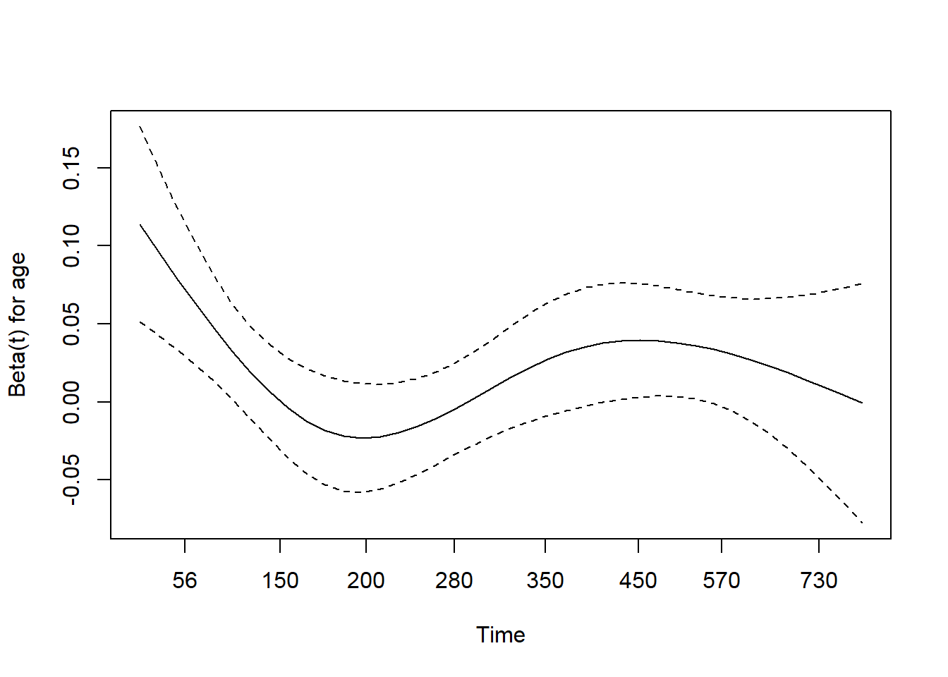

plot(zp1[1], resid=FALSE)

8.3.7.2 Check additivity

Interaction not significant $\rightarrow$ additivity

cfitm<-update(cfit, . ~ . + age*sex)
anova(cfit, cfitm)

## Analysis of Deviance Table
##  Cox model: response is  Surv(time, status)
##  Model 1: ~ age + sex + wt.loss
##  Model 2: ~ age + sex + wt.loss + age:sex
##    loglik  Chisq Df Pr(>|Chi|)
## 1 -673.06                     
## 2 -672.88 0.3473  1     0.5557

8.3.7.3 Check linearity

Non-linearity not significant.

cfitl<-coxph(Surv(time, status) ~ pspline(age) + sex + wt.loss, lung)
print(cfitl, digit=3)

## Call:
## coxph(formula = Surv(time, status) ~ pspline(age) + sex + wt.loss, 
##     data = lung)
## 
##                          coef se(coef)      se2    Chisq   DF      p
## pspline(age), linear  0.02011  0.00931  0.00931  4.66393 1.00 0.0308
## pspline(age), nonlin                             3.02601 3.08 0.4018
## sex                  -0.53145  0.17549  0.17513  9.17105 1.00 0.0025
## wt.loss               0.00056  0.00619  0.00618  0.00818 1.00 0.9279
## 
## Iterations: 4 outer, 12 Newton-Raphson
##      Theta= 0.799 
## Degrees of freedom for terms= 4.1 1.0 1.0 
## Likelihood ratio test=18.4  on 6.07 df, p=0.006
## n= 214, number of events= 152 
##    (14 observations deleted due to missingness)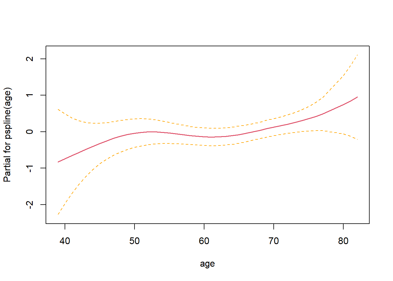

#Plot effect of age (quite linear)   
termplot(cfitl, term=1, se=TRUE)

8.3.7.4 Formatting Cox regression results

library(knitr)
#tidy function from the broom package
broom::tidy(
  cfit2, 
  exp = TRUE) %>% 
  kable()

term	estimate	std.error	statistic	p.value
sex	0.598566	0.1674580	-3.064760	0.0021784
age	1.017191	0.0092233	1.848078	0.0645910

#tbl_regression from the gtsummary package
#install.packages("gtsummary")
#library(gtsummary)
#cfit2 %>% 
#  gtsummary::tbl_regression(exp = TRUE)

8.3.8 Transform survival curves: plot cumulative events and cumulative hazard function

#plot cumulative event (incidence)
ggsurvplot(fit2, conf.int = TRUE,
           fun = "event",
           risk.table = TRUE, risk.table.col = "strata")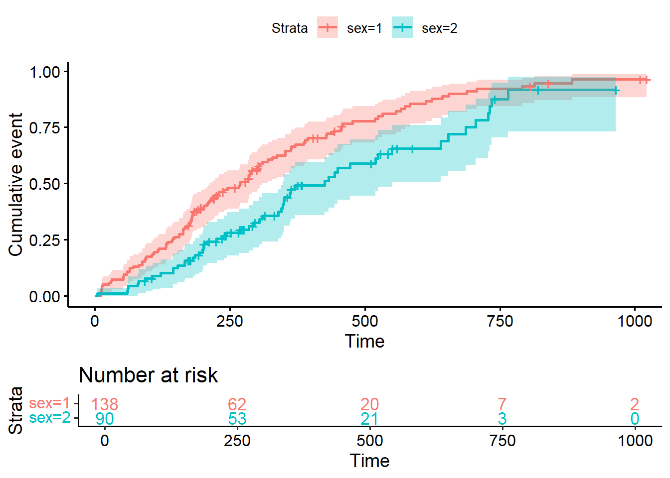

#Plot the cumulative hazard function
ggsurvplot(fit2, conf.int = TRUE,
           fun = "cumhaz",
           risk.table = TRUE, risk.table.col = "strata")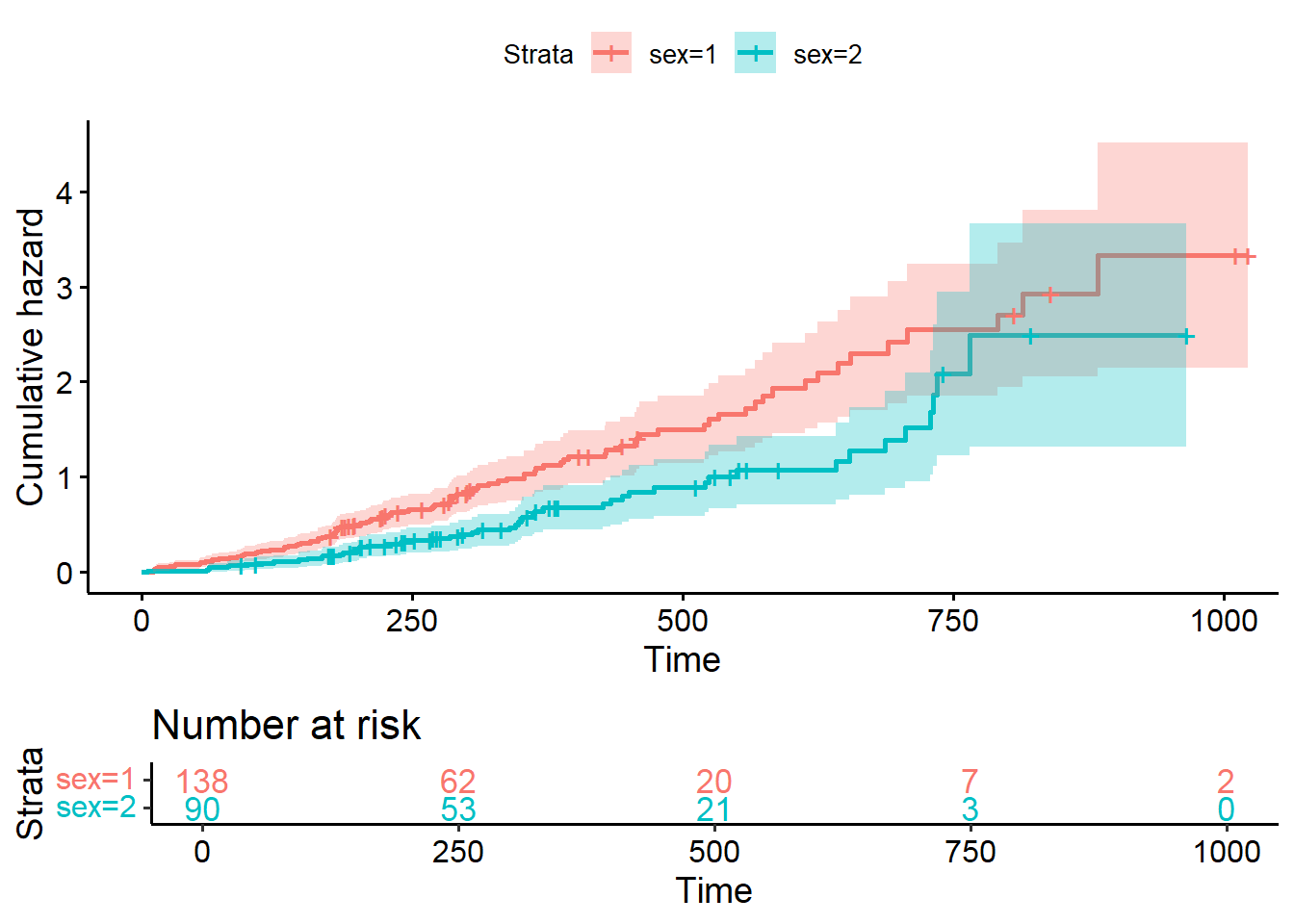

8.3.9 More advanced aspects in survival analysis

8.3.9.1 Time Dependent Covariates

8.3.9.1.1 Background

Log-rank tests and Cox regression to examine associations between survival outcomes and covariates of interest at baseline (before follow-up time for the event begins).
Covariate that is measured after follow-up time begin $\rightarrow$ time dependent covariate

8.3.9.1.2 Landmark Analysis Method

Select a fixed time after baseline as your landmark time. Note: this should be done based on clinical information, prior to data inspection
Subset population for those followed at least until landmark time. Note: always report the number excluded due to the event of interest or censoring prior to the landmark time.
Calculate follow-up from landmark time and apply traditional log-rank tests or Cox regression

8.3.9.1.3 Example Heart transplant data

Naive analysis showed patients who received heart transplants lived significantly longer than those who did not.

$\rightarrow$ Problems:

Transplant is a time dependent covariate; patients who received a transplant had to live long enough to receive that transplant.
The analysis only shows that patients who live long enough to receive a transplant have longer lives than patients who don’t live as long ( $\rightarrow$ tautology)

fit.n<-coxph(Surv(futime, fustat) ~ transplant + age + surgery, data=jasa)
summary(fit.n)

## Call:
## coxph(formula = Surv(futime, fustat) ~ transplant + age + surgery, 
##     data = jasa)
## 
##   n= 103, number of events= 75 
## 
##                coef exp(coef) se(coef)      z Pr(>|z|)    
## transplant -1.71711   0.17958  0.27853 -6.165 7.05e-10 ***
## age         0.05889   1.06065  0.01505  3.913 9.12e-05 ***
## surgery    -0.41902   0.65769  0.37118 -1.129    0.259    
## ---
## Signif. codes:  0 '***' 0.001 '**' 0.01 '*' 0.05 '.' 0.1 ' ' 1
## 
##            exp(coef) exp(-coef) lower .95 upper .95
## transplant    0.1796     5.5684    0.1040     0.310
## age           1.0607     0.9428    1.0298     1.092
## surgery       0.6577     1.5205    0.3177     1.361
## 
## Concordance= 0.732  (se = 0.031 )
## Likelihood ratio test= 45.85  on 3 df,   p=6e-10
## Wald test            = 47.15  on 3 df,   p=3e-10
## Score (logrank) test = 52.63  on 3 df,   p=2e-11

8.3.9.1.4 Landmark analysis example for heart transplant data

Set a landmark at 30 days
Divide patients into two groups: patients who receive the intervention prior to the landmark go into the intervention group and those who did not are placed in the comparison group.
Select patients who lived at least 30 days (79 of the 103 patients lived this long). Of these 79 patients, 33 had a transplant within 30 days, and 46 did not. Of these 46, 30 subsequently had a heart transplant, but we still count them in the “no transplant within 30 days” group.
Created a variable (we shall call it “transplant30”) which has a fixed value (that is, it does not change over time) for all patients in our set of 30-day survivors.
$\rightarrow$ there is no difference in survival between those who got a transplant and those who did not.
Issues: a) When to set the landmark?; b) Exclude a lot of data (only patients who survive up to the landmark are included in the study);
1. all patients (in particular, those in the comparison group) remain in their originally assigned group regardless of what happens in the future, i.e., after the landmark

ind30 <- jasa$futime >= 30
transplant30 <- {{jasa$transplant == 1} & {jasa$wait.time < 30}}
summary(coxph(Surv(futime, fustat) ~ transplant30 + age + surgery, data=jasa, subset=ind30 ))

## Call:
## coxph(formula = Surv(futime, fustat) ~ transplant30 + age + surgery, 
##     data = jasa, subset = ind30)
## 
##   n= 79, number of events= 52 
## 
##                      coef exp(coef) se(coef)      z Pr(>|z|)  
## transplant30TRUE -0.04214   0.95874  0.28377 -0.148   0.8820  
## age               0.03720   1.03790  0.01714  2.170   0.0300 *
## surgery          -0.81966   0.44058  0.41297 -1.985   0.0472 *
## ---
## Signif. codes:  0 '***' 0.001 '**' 0.01 '*' 0.05 '.' 0.1 ' ' 1
## 
##                  exp(coef) exp(-coef) lower .95 upper .95
## transplant30TRUE    0.9587     1.0430    0.5497    1.6720
## age                 1.0379     0.9635    1.0036    1.0734
## surgery             0.4406     2.2697    0.1961    0.9898
## 
## Concordance= 0.618  (se = 0.044 )
## Likelihood ratio test= 9.5  on 3 df,   p=0.02
## Wald test            = 8.61  on 3 df,   p=0.03
## Score (logrank) test = 8.94  on 3 df,   p=0.03

8.3.9.2 Model time depedent covariate

Can be done in the framework of the classical Cox proportional hazards model, but important adjustments to data is required: pre-processing the data into “start-stop” format. Example heart transplant data:

Divides the time data for patients who had a heart transplant into two time periods, one before the transplant and one after.
Use tmerge function to create “start-stop” format.

jasaid<-data.frame(id=rownames(jasa), jasa)
# extract some example patients
heart.s<-jasaid[c(2, 5, 10, 12, 28,95), c("id","wait.time","futime","fustat","transplant")]
heart.s

##    id wait.time futime fustat transplant
## 2   2        NA      5      1          0
## 5   5        NA     17      1          0
## 10 10        11     57      1          1
## 12 12        NA      7      1          0
## 28 28        70     71      1          1
## 95 95         1     15      1          1

dat.td<-tmerge(heart.s, heart.s, id=id, death=event(futime, fustat), transpl=tdc(wait.time))
kable(dat.td)

id	wait.time	futime	fustat	transplant	tstart	tstop	death	transpl
2	NA	5	1	0	0	5	1	0
5	NA	17	1	0	0	17	1	0
10	11	57	1	1	0	11	0	0
10	11	57	1	1	11	57	1	1
12	NA	7	1	0	0	7	1	0
28	70	71	1	1	0	70	0	0
28	70	71	1	1	70	71	1	1
95	1	15	1	1	0	1	0	0
95	1	15	1	1	1	15	1	1

summary(coxph(Surv(tstart, tstop, death) ~ transpl,data=dat.td))

## Call:
## coxph(formula = Surv(tstart, tstop, death) ~ transpl, data = dat.td)
## 
##   n= 9, number of events= 6 
## 
##           coef exp(coef) se(coef)     z Pr(>|z|)
## transpl 0.2846    1.3292   0.9609 0.296    0.767
## 
##         exp(coef) exp(-coef) lower .95 upper .95
## transpl     1.329     0.7523    0.2021      8.74
## 
## Concordance= 0.5  (se = 0.082 )
## Likelihood ratio test= 0.09  on 1 df,   p=0.8
## Wald test            = 0.09  on 1 df,   p=0.8
## Score (logrank) test = 0.09  on 1 df,   p=0.8

8.3.9.3 Repeated events

Examples: time from treatment to seizure episodes (multiple repeated seizure episodes may occur); infections in transplanted patients
Need to reformat data to “start, stop” form Example data of Children with chronic granulotomous disease (cgd0).

fit.re<-coxph(Surv(tstart, tstop, status) ~ treat, data=cgd)
summary(fit.re)

## Call:
## coxph(formula = Surv(tstart, tstop, status) ~ treat, data = cgd)
## 
##   n= 203, number of events= 76 
## 
##                coef exp(coef) se(coef)      z Pr(>|z|)    
## treatrIFN-g -1.0953    0.3344   0.2610 -4.196 2.71e-05 ***
## ---
## Signif. codes:  0 '***' 0.001 '**' 0.01 '*' 0.05 '.' 0.1 ' ' 1
## 
##             exp(coef) exp(-coef) lower .95 upper .95
## treatrIFN-g    0.3344       2.99    0.2005    0.5578
## 
## Concordance= 0.629  (se = 0.029 )
## Likelihood ratio test= 20.11  on 1 df,   p=7e-06
## Wald test            = 17.61  on 1 df,   p=3e-05
## Score (logrank) test = 19.42  on 1 df,   p=1e-05

8.4 Practice

Use the dataframe “nafld1” of dataset “ndfld” of the “survival” package:

Plot the overall survival curve, estimate median survival time, estimate survival at 1.5 year
Plot the survival curves of males and females, test the difference between the curves
Examine each of other covariates (age, weight, height, bmi) and check if any covariate significantly affect survival
Report and provide rationale for the best multivariate Cox model.

8.5 Reference materials

8.5.1 Books, other resources

Tutorial for the essential R package which is the base of most packages related to survival analysis: survival.
Comprehensive book: Applied Survival Analysis Using R.

8.5.2 Online tutorials

References

Kassambara, Alboukadel, Marcin Kosinski, and Przemyslaw Biecek. 2024. Survminer: Drawing Survival Curves Using Ggplot2. https://rpkgs.datanovia.com/survminer/index.html.

Moore, Dirk F. 2016. Applied Survival Analysis Using r. Springer Cham.

Spinu, Vitalie, Garrett Grolemund, and Hadley Wickham. 2024. Lubridate: Make Dealing with Dates a Little Easier. https://lubridate.tidyverse.org.

Therneau, Terry M. 2024. Survival: Survival Analysis. https://github.com/therneau/survival.

id	wait.time	futime	fustat	transplant	tstart	tstop	death	transpl
2	NA	5	1	0	0	5	1	0
5	NA	17	1	0	0	17	1	0
10	11	57	1	1	0	11	0	0
10	11	57	1	1	11	57	1	1
12	NA	7	1	0	0	7	1	0
28	70	71	1	1	0	70	0	0
28	70	71	1	1	70	71	1	1
95	1	15	1	1	0	1	0	0
95	1	15	1	1	1	15	1	1

id	wait.time	futime	fustat	transplant	tstart	tstop	death	transpl
2	NA	5	1	0	0	5	1	0
5	NA	17	1	0	0	17	1	0
10	11	57	1	1	0	11	0	0
10	11	57	1	1	11	57	1	1
12	NA	7	1	0	0	7	1	0
28	70	71	1	1	0	70	0	0
28	70	71	1	1	70	71	1	1
95	1	15	1	1	0	1	0	0
95	1	15	1	1	1	15	1	1

id	wait.time	futime	fustat	transplant	tstart	tstop	death	transpl
2	NA	5	1	0	0	5	1	0
5	NA	17	1	0	0	17	1	0
10	11	57	1	1	0	11	0	0
10	11	57	1	1	11	57	1	1
12	NA	7	1	0	0	7	1	0
28	70	71	1	1	0	70	0	0
28	70	71	1	1	70	71	1	1
95	1	15	1	1	0	1	0	0
95	1	15	1	1	1	15	1	1