Chapter 9 Longitudinal Data Analysis with R

Ho Thi Nhan, MD, PhD

9.1 Longitudinal studies

• Collect data on the same individuals repeatedly over time

9.1.1 Benefits

Advantages of longitudinal studies as compared to cross-sectional studies:

• Record incident events
• Ascertain exposure prospectively
• Separate time effects: cohort, period, age
• Distinguish changes over time within individuals
• Help establish causal effect of exposure on outcome
  
• Repeated measures over time of the same subjects.

9.1.2 Separate time effects: cohort, period, age

9.1.2.1 Cohort effects

• Differences between individuals at baseline
• “Level”
• Example: Younger individuals begin at a higher level

9.1.2.2 Age effects

• Differences within individuals over time
• “Trend”
• Example: Outcomes increase over time for everyone

9.1.2.3 Period Effects

• Measurement date varies => measured outcomes/exposures varies

9.1.3 Distinguish changes over time within individuals

Age can be partitioned into two components:

• Cross-sectional comparison: $E[Y_{i1}]$ = $\beta_{0}$ + $\beta_{C}x_{i1}$
• Longitudinal comparison: $E[Y_{ij} - Y_{i1}]$ = $\beta_{L}(x_{ij}-x_{i1})$ for observation j = 1,…,mi on subject i = 1,…,n. 
• Putting these two models together: $E[Y_{ij}]$ = $\beta_{0}$ + $\beta_{C}x_{i1}$ + $\beta_{L}(x_{ij}-x_{i1})$
• $\beta_{L}$ represents the expected change in the outcome per unit change in age for a given subject.

9.1.4 Longitudinal vs. cross-sectional

For comparison of groups A and B:

• Cross-sectional:

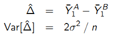
• Longitudinal:

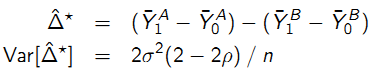
• Benefits of Longitudinal estimate: may be more precise, may reduce bias because each subject “acts as their own control”.

9.1.5 Challenges

• Determine causality when covariates vary over time
• Choose exposure lag when covariates vary over time
• Account for incomplete participant follow-up
• Require specialized methods that account for longitudinal correlation

9.1.6 Longitudinal correlation

Repeated measures over time are correlated. Ignoring dependence may lead to incorrect inference:

• Longitudinal correlation usually positive
• Estimated standard errors may be too small
• Confidence intervals are too narrow; too often exclude true value.

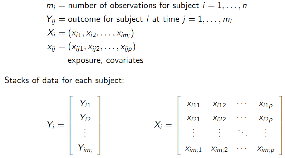
9.2 Example: Bangladesh data

This is a published data from a cohort study of 50 healthy Bangladeshi infants.

#load multiple packages
packages<-c("rio","tidyverse","knitr","lme4","mgcv","geepack","gee","ggplot2","sjPlot","sjlabelled","sjmisc") #,"longCatEDA"
lapply(packages, library, character.only = TRUE)

#import sheet 2 only
sh2<-import("./metamicrobiomeR-master/inst/extdata/QIIME_outputs/Bangladesh/nature13421-s2.xlsx",sheet=2,skip=1)

#Rename column names
oldname<-colnames(sh2)
newname<-c("cohort",
           "family.id",
           "child.id",
           "sample.id",
           "age.d",
           "age.m",
           "whz","waz","haz",
           "breast.milk",
           "formula",
           "solid",
           "diarrhea",
           "antibiotic.7d",
           "medication",
           "no.sequence",
           "serun.id",
           "barcode")
sh2<-sh2 %>% rename_at(vars(oldname), ~newname)
#colnames(sh2)
#remove unused rows 
sh2<-sh2 %>% 
  filter(!is.na(family.id))
#View(sh2)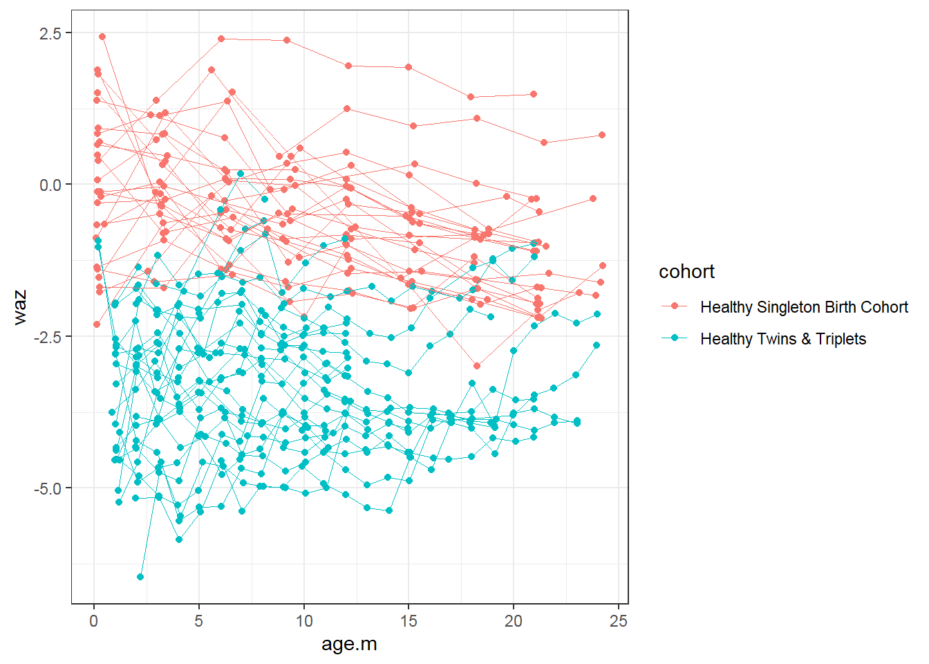

9.2.1 Longitudinal data visualization: Spaghetti plot

For continuous variables.

sh2 %>%
  filter(!is.na(whz)) %>%
  ggplot()+ 
  geom_point(aes(x = age.m, y = waz, group = child.id, colour=cohort))+
  geom_line(aes(x = age.m, y = waz, group = child.id, colour=cohort),size=0.3)

9.2.2 Plot mean

sh2 %>%
  filter(!is.na(whz)) %>%
  mutate(age.m.r=round(age.m,0)) %>%
  group_by(age.m.r, cohort)%>%
  summarise(mean.waz=mean(waz,na.rm=T)) %>%
  ggplot()+ 
  geom_point(aes(x = age.m.r, y = mean.waz, colour=cohort))+
  geom_line(aes(x = age.m.r, y = mean.waz, colour=cohort),size=0.3) 

9.3 Options for analysis of change

Does mean change differ across groups?

9.3.1 Pre-post analysis

• Same baseline (e.g.randomization): analysis of post or change
• Different baseline: analysis of post or change adjusting for baseline

=> Simple pre-post data don’t incorporate correlation within individuals.

9.3.2 Longitudinal regression models

GEE and mixed-effects models Gałecki and Burzykowski (2013):

• Exploratory data analysis
• Regression model specification
• Parameter interpretation
• Covariance and correlation

9.3.3 Longitudinal data definition

Data definition:

9.4 Exploratory data analysis

9.4.1 Summarize mean and covariance structure

• Summary statistics over time (by groups)
• Individual plots of observed and fitted values
• Empirical covariance structure (variance and correlation)

9.4.2 Main points

• Show as much of the data as possible, rather than only summaries
• Highlight aggregate patterns of potential scientific interest
• Identify both cross-sectional and longitudinal patterns
• Facilitate the identification of unusual individuals or observations

9.4.3 Longitudinal data visualization: Spaghetti plot

For continuous variables:

sh2 %>%
  filter(!is.na(whz)) %>%
  ggplot()+ 
  geom_point(aes(x = age.m, y = waz, group = child.id, colour=cohort))+
  geom_line(aes(x = age.m, y = waz, group = child.id, colour=cohort),size=0.3)

9.4.4 Plot mean

On average…

• Trend: Weight for age z score (waz) decreases over time for singletons; not change in twins-triplets
• Cross-sectional: singletons have larger waz than twins-triplets at every age
• Longitudinal: Decrease in average waz is larger for singletons

d1<-sh2 %>%
  filter(!is.na(whz)) %>%
  mutate(age.m.r=round(age.m,0)) %>%
  group_by(age.m.r, cohort)%>%
  summarise(mean.waz=mean(waz,na.rm=T)) 
d1 %>%
  ggplot()+ 
  geom_point(aes(x = age.m.r, y = mean.waz, colour=cohort))+
  geom_line(aes(x = age.m.r, y = mean.waz, colour=cohort),size=0.3)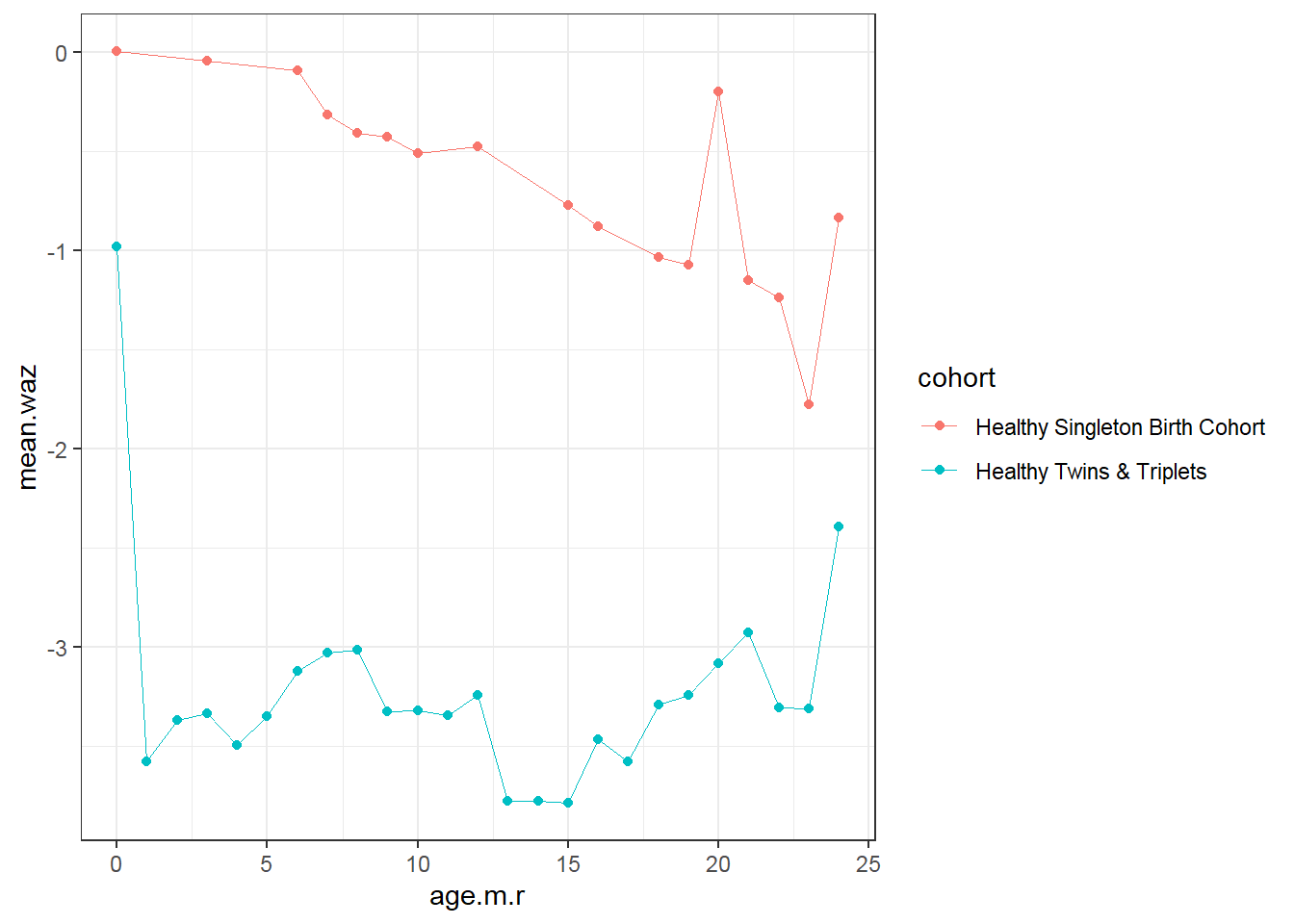 

9.4.5 Linear model for time

9.4.5.1 Mean Model

time=age or “age.m” in this data:

$E[Y_{ij}|age_{ij}]$= $\beta_{0} + \beta_{1}age_{ij}$

Rate of Change - Slope of the curve $\beta_{1}$ - Constant rate of change

9.4.5.2 Other models for time

• Quadratic
• Linear spline
• Cubic spline
• Higher-order polynomials

9.4.5.3 Research question

• Rate of change = time slope $E[waz_{ij}|x_{ij} = (age.m, cohort)]$ = $\beta_{0}(x_{ij}) + \beta_{1}(x_{ij})time_{ij}$

fitlm1<-lm(waz~age.m, data=sh2)
summary(fitlm1)

## 
## Call:
## lm(formula = waz ~ age.m, data = sh2)
## 
## Residuals:
##    Min     1Q Median     3Q    Max 
## -4.134 -1.446 -0.114  1.333  4.758 
## 
## Coefficients:
##              Estimate Std. Error t value Pr(>|t|)    
## (Intercept) -2.323415   0.134893 -17.224   <2e-16 ***
## age.m       -0.005831   0.011508  -0.507    0.613    
## ---
## Signif. codes:  0 '***' 0.001 '**' 0.01 '*' 0.05 '.' 0.1 ' ' 1
## 
## Residual standard error: 1.742 on 571 degrees of freedom
##   (423 observations deleted due to missingness)
## Multiple R-squared:  0.0004494,  Adjusted R-squared:  -0.001301 
## F-statistic: 0.2567 on 1 and 571 DF,  p-value: 0.6126

• Does the rate of change differ between singletons vs. twins-triplets? $E[Y_{ij}]$ = $\beta_{0} + \beta_{1}age_{ij} + \beta_{2}cohort_{i} + \beta_{3}age_{ij}*cohort_{i}$

fitlm2<-lm(waz~age.m +cohort +age.m*cohort, data=sh2)
summary(fitlm2)

## 
## Call:
## lm(formula = waz ~ age.m + cohort + age.m * cohort, data = sh2)
## 
## Residuals:
##     Min      1Q  Median      3Q     Max 
## -3.1604 -0.7730 -0.1336  0.7111  3.4986 
## 
## Coefficients:
##                                      Estimate Std. Error t value Pr(>|t|)    
## (Intercept)                           0.11060    0.14276   0.775 0.438815    
## age.m                                -0.05676    0.01110  -5.113 4.34e-07 ***
## cohortHealthy Twins & Triplets       -3.41607    0.17838 -19.150  < 2e-16 ***
## age.m:cohortHealthy Twins & Triplets  0.05487    0.01469   3.734 0.000207 ***
## ---
## Signif. codes:  0 '***' 0.001 '**' 0.01 '*' 0.05 '.' 0.1 ' ' 1
## 
## Residual standard error: 1.096 on 569 degrees of freedom
##   (423 observations deleted due to missingness)
## Multiple R-squared:  0.6055, Adjusted R-squared:  0.6034 
## F-statistic: 291.1 on 3 and 569 DF,  p-value: < 2.2e-16

9.4.5.4 Parameter interpretation

• $\beta_{1}$ = expected waz change (per month) for singletons (reference group)
• $\beta_{2}$ = expected difference in waz comparing twins_triplets to singletons at first visit (newborn)
• $\beta_{3}$ = expected difference in waz change (per month) between twins_triplets and singletons

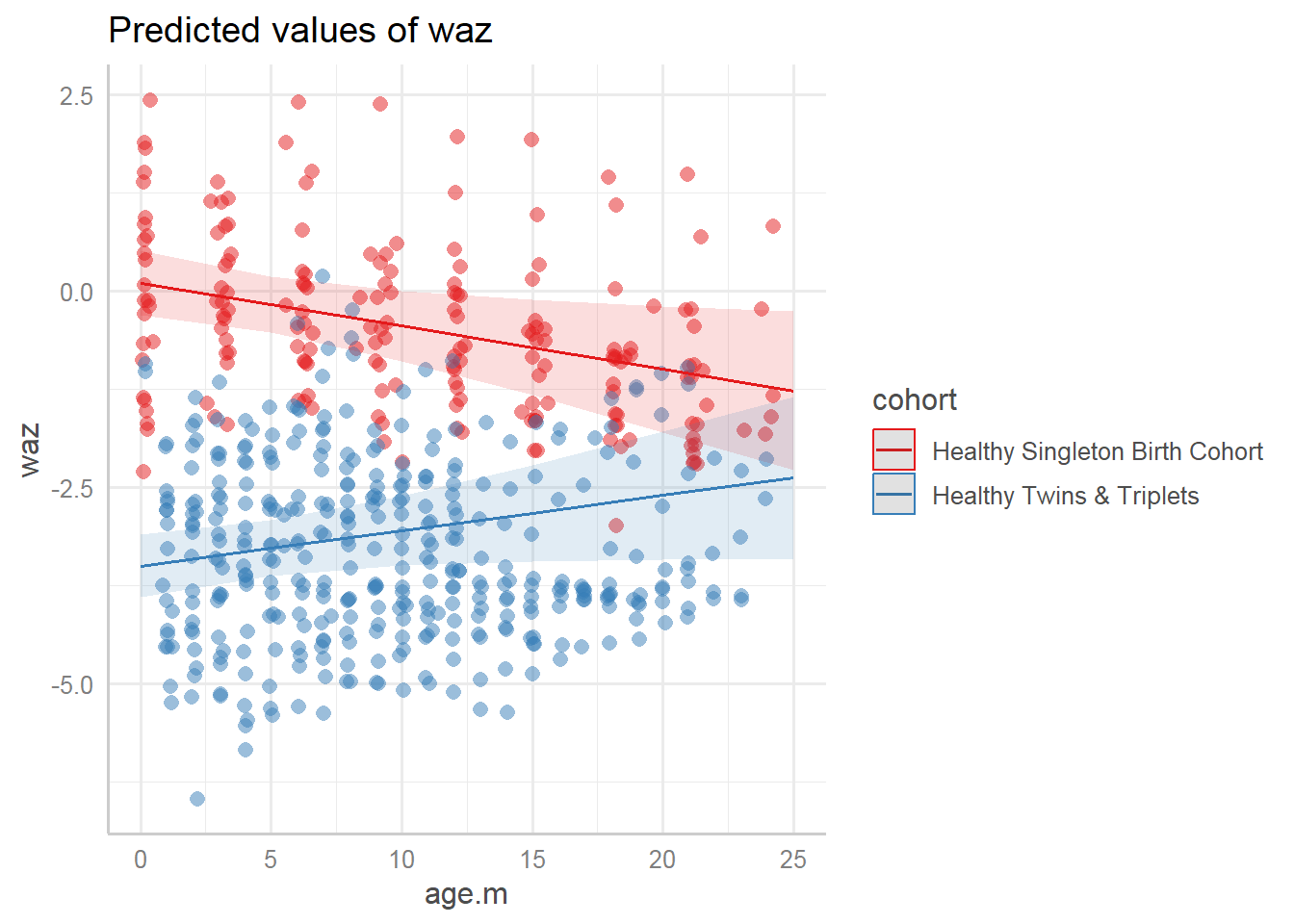
9.4.5.5 Plot with linear regression line

Using “glm” => ignore longitudinal data.

sh2 %>%
  filter(!is.na(whz)) %>%
  ggplot()+ 
  geom_point(aes(x = age.m, y = waz, group = child.id, colour=cohort))+
  geom_line(aes(x = age.m, y = waz, group = child.id, colour=cohort),size=0.3)+
  stat_smooth(aes(x = age.m, y = waz, colour=cohort), method = 'glm',size=2)+
  geom_point(aes(x = age.m.r, y = mean.waz, colour=cohort), size=4, pch=17,data=d1)+
  geom_line(aes(x = age.m.r, y = mean.waz, colour=cohort),size=2,pch=17,data=d1)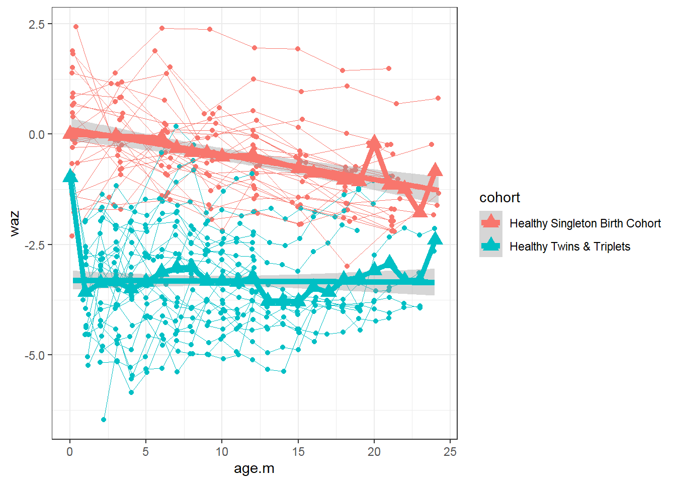 

9.4.6 Issues of linear model

The below are not accounted.

9.4.6.1 Dependence & Correlation

Response variables measured on the same subject are correlated. - Observations are dependent or correlated when one variable does predict the value of another variable (waz at month 1 may predict waz at month 2)

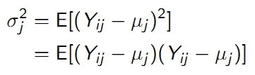
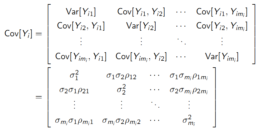
9.4.6.2 Variance

The variance measures the average distance that an observation falls away from the mean. The variance of a variable $Y_{ij}$ (fix time j) is defined as:

9.4.6.3 Covariance

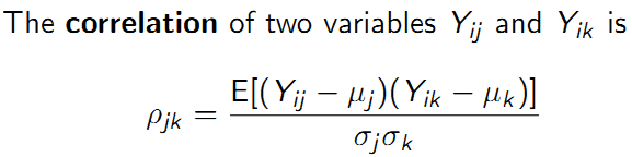
• The covariance measures whether, on average, departures in one variable $Y_{ij}-\mu_{j}$ ‘go together with’ departures in a second variable $Y_{ik}-\mu_{k}$.

• The covariance of two variables $Y_{ij}$ and $Y_{ik}$ is: $\sigma_{jk}$ = $E[(Y_{ij}-\mu_{j})(Y_{ik}-\mu_{k})]$

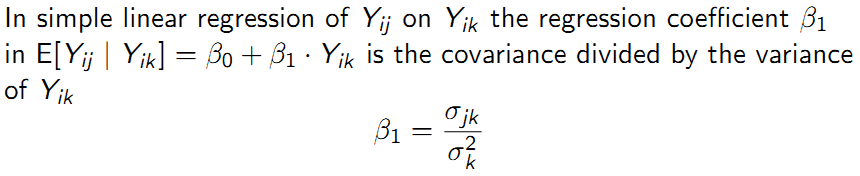
• Simple linear regression covariance:

9.4.6.4 Correlation

• The correlation is a measure of dependence that takes values between -1 and +1
• A correlation of 0 implies that two measures are unrelated (linearly)
• A correlation of 1 implies that the two measures fall perfectly on a line (one exactly predicts the other!)
• Correlation formula:

9.4.7 What to add to model

9.4.7.1 Covariance

Variance Covariance matrix:

9.5 Generalized estimating equations (GEE)

9.5.1 GEE: example Bangladesh data

Characterize waz change among singletons and twins-triplets:

• 1. Estimate the average waz change among all children
• 2. Estimate the waz change for individual children
• 3. Characterize the degree of heterogeneity across children
• 4. Identify factors that predict waz change

9.5.2 Introduction to GEE

Contrast average outcome values across populations of individuals defined by covariate values, while accounting for correlation.

• Focus on a generalized linear model with regression parameters $\beta$, which characterize the systemic variation in Y across covariates X.

• Longitudinal correlation structure is a nuisance feature of the data.

9.5.3 Assumptions

• Observations are independent across subjects
• Observations may be correlated within subjects

9.5.4 Mean model

Primary focus of the analysis:

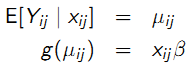
• May correspond to any generalized linear model with link g(.)

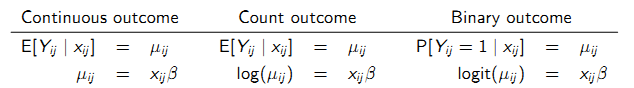
• Characterizes a marginal mean regression model

9.5.5 Marginal mean

Definition: $\mu_{ij}$ does not condition on anything other than $x_{ij}$ . Mixed effect and transition model:

9.5.6 Covariance model

Longitudinal correlation is a nuisance; secondary to mean model of interest.

• Assume a form for variance that may depend on $\mu_{ij}$ which may also include a scale or dispersion parameter $\phi$ > 0.

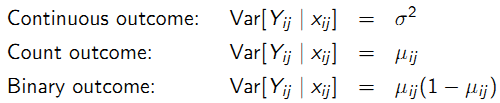
• Select a model for longitudinal correlation with parameters $\alpha$.

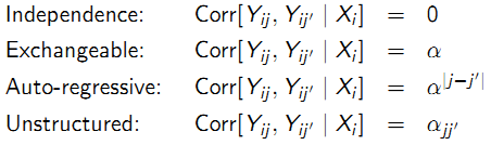
9.5.7 Correlation models

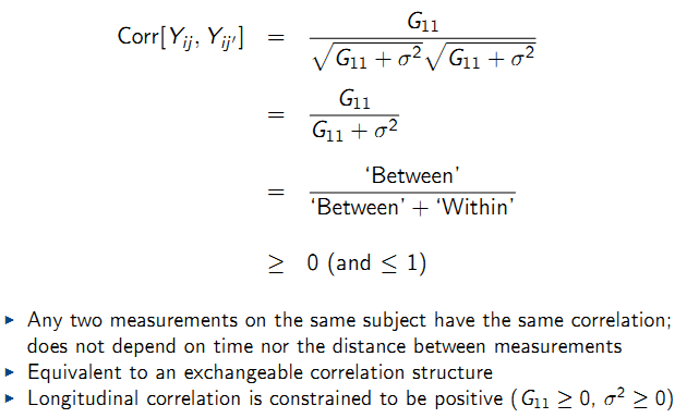
Correlation between any two observations on the same subject:

• Independence: is assumed to be zero (observations over time are independent). Always appropriate with use of robust variance estimator (large n)
• Exchangeable: is assumed to be constant (all observations over time have the same correlation). More appropriate for clustered data
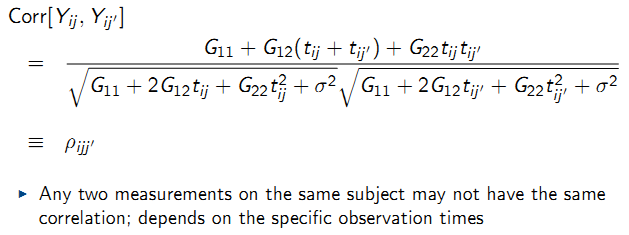
• Auto-regressive: is assumed to depend on time or distance (correlation decreases as a power of how many timepoints apart two observations are). More appropriate for equally-spaced longitudinal data
• Unstructured: is assumed to be distinct for each pair (correlation between all timepoints may be different). Only appropriate for short series (small m) on many subjects (large n)

9.5.8 Semi-parametric

• Specification of a mean model and correlation model does not identify a complete probability model for the outcomes
• The [mean, correlation] model is semi-parametric because it only specifies the first two moments of the outcomes
• Additional assumptions are required to identify a complete probability model and a corresponding parametric likelihood function (GLMM)

Note: Construct an unbiased estimating function to estimate $\beta$ and generate valid statistical inference, while accounting for correlation.

9.5.9 Generalized estimating equations: Intuition

Generalized estimating equations: Intuition

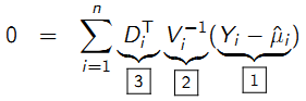
• [1] The model for the mean, $\mu_{i}(\beta)$, is compared to the observed data, $Y_{i}$; setting the equations to equal 0 tries to minimize the difference between observed and expected.
• [2] Estimation uses the inverse of the variance (covariance) to weight the data from subject i ; more weight is given to differences between observed and expected for those subjects who contribute more information
• [3] This is simply a ‘change of scale’ from the scale of the mean, $\mu_{i}(\beta)$, to the scale of the regression coefficients (covariates)

9.5.10 Properties of $\hat{\beta}$

• $\hat{\beta}$ is a consistent estimator for $\beta$ even if the model for longitudinal correlation is incorrectly specified, i.e. $\hat{\beta}$ is ‘robust’ to correlation model mis-specification
• However, the variance of $\hat{\beta}$ must capture the correlation in the data, either by choosing the correct correlation model, or via an alternative variance estimator
• Selecting an approximately correct correlation model will yield a more efficient estimator for $\beta$, i.e. $\hat{\beta}$ has the smallest variance (standard error) if the correlation model is correctly specified

9.5.11 GEE: comments

• GEE is specified by a mean model and a correlation model

1. A regression model for the average outcome, e.g. linear, logistic;
2. A model for longitudinal correlation, e.g. independence, exchangeable

• GEE also computes an empirical variance estimator (aka sandwich, robust, or Huber-White variance estimator)
• Empirical variance estimator provides valid standard errors for $\hat{\beta}$ even if the correlation model is incorrect, but requires n >= 40 and n >> m.

Note: Although the correlation model does not need to be correctly specified to obtain a consistent estimator for $\beta$ or valid standard errors for $\hat{\beta}$, selecting a non-independence or weighted correlation structure permits use of the model-based variance estimator and may provide improved efficiency for $\hat{\beta}$.

9.5.12 Inference for $\beta$

• Wald test
• Note: Likelihood ratio test not available; not relied on a likelihood function

9.5.13 GEE: example Bangladesh data

9.5.13.1 Objectives

Characterize waz change among singletons and twins-triplets:

• 1. Estimate the average waz change among all children
• 2. Estimate the waz change for individual children
• 3. Characterize the degree of heterogeneity across children
• 4. Identify factors that predict waz change

9.5.13.2 Approach

• Examine waz change among twins_triplets and singletons: $E[Y_{ij}]$ = $\beta_{0} + \beta_{1}age_{ij} + \beta_{2}cohort{i} + \beta_{3}age_{ij}*cohort_{i}$
• Consider various specifications for the ‘working’ correlation structure:

1. Independence;
2. Exchangeable;
3. Auto-regressive;
4. Unstructured;

• Selection of a working correlation structure should be guided by a prior knowledge and/or exploratory analysis

9.5.13.3 GEE trying different correlation structure

This may be done with “geepack” package (Højsgaard, Halekoh, and Yan 2024):

#library(geepack)
waz.nona<-sh2 %>%
  filter(!is.na(waz))
g.i<-geeglm(waz~age.m +cohort +age.m*cohort, id=child.id,corstr="independence", data=waz.nona)
summary(g.i)

## 
## Call:
## geeglm(formula = waz ~ age.m + cohort + age.m * cohort, data = waz.nona, 
##     id = child.id, corstr = "independence")
## 
##  Coefficients:
##                                        Estimate    Std.err      Wald Pr(>|W|)    
## (Intercept)                           1.106e-01  4.463e-16 6.141e+28   <2e-16 ***
## age.m                                -5.676e-02  4.174e-17 1.849e+30   <2e-16 ***
## cohortHealthy Twins & Triplets       -3.416e+00  7.189e-17 2.258e+33   <2e-16 ***
## age.m:cohortHealthy Twins & Triplets  5.487e-02  3.328e-18 2.718e+32   <2e-16 ***
## ---
## Signif. codes:  0 '***' 0.001 '**' 0.01 '*' 0.05 '.' 0.1 ' ' 1
## 
## Correlation structure = independence 
## Estimated Scale Parameters:
## 
##             Estimate   Std.err
## (Intercept)    1.193 3.975e-17
## Number of clusters:   1  Maximum cluster size: 573

g.e<-geeglm(waz~age.m +cohort +age.m*cohort, id=child.id,corstr="exchangeable", data=waz.nona)
summary(g.e)

## 
## Call:
## geeglm(formula = waz ~ age.m + cohort + age.m * cohort, data = waz.nona, 
##     id = child.id, corstr = "exchangeable")
## 
##  Coefficients:
##                                      Estimate Std.err Wald Pr(>|W|)
## (Intercept)                            0.1106     NaN  NaN      NaN
## age.m                                 -0.0568     NaN  NaN      NaN
## cohortHealthy Twins & Triplets        -3.4161     NaN  NaN      NaN
## age.m:cohortHealthy Twins & Triplets   0.0549     NaN  NaN      NaN
## 
## Correlation structure = exchangeable 
## Estimated Scale Parameters:
## 
##             Estimate  Std.err
## (Intercept)     1.19 1.04e-16
##   Link = identity 
## 
## Estimated Correlation Parameters:
##       Estimate  Std.err
## alpha -0.00175 3.39e-19
## Number of clusters:   1  Maximum cluster size: 573

g.a<-geeglm(waz~age.m +cohort +age.m*cohort, id=child.id,corstr="ar1", data=waz.nona)
summary(g.a)

## 
## Call:
## geeglm(formula = waz ~ age.m + cohort + age.m * cohort, data = waz.nona, 
##     id = child.id, corstr = "ar1")
## 
##  Coefficients:
##                                       Estimate   Std.err     Wald Pr(>|W|)    
## (Intercept)                          -4.99e-02  1.96e-06 6.47e+08   <2e-16 ***
## age.m                                -5.45e-02  1.23e-09 1.96e+15   <2e-16 ***
## cohortHealthy Twins & Triplets       -3.51e+00  2.38e-06 2.17e+12   <2e-16 ***
## age.m:cohortHealthy Twins & Triplets  8.53e-02  4.48e-08 3.62e+12   <2e-16 ***
## ---
## Signif. codes:  0 '***' 0.001 '**' 0.01 '*' 0.05 '.' 0.1 ' ' 1
## 
## Correlation structure = ar1 
## Estimated Scale Parameters:
## 
##             Estimate  Std.err
## (Intercept)     1.23 3.08e-07
##   Link = identity 
## 
## Estimated Correlation Parameters:
##       Estimate  Std.err
## alpha    0.827 2.13e-07
## Number of clusters:   1  Maximum cluster size: 573

#g.u<-geeglm(waz~age.m +cohort +age.m*cohort, id=child.id,corstr="unstructured", data=waz.nona)
#summary(g.u)
#OLS
#=> SE are larger 
fit.ols<-lm(waz~age.m +cohort +age.m*cohort,data=waz.nona)
summary(fit.ols)

## 
## Call:
## lm(formula = waz ~ age.m + cohort + age.m * cohort, data = waz.nona)
## 
## Residuals:
##    Min     1Q Median     3Q    Max 
## -3.160 -0.773 -0.134  0.711  3.499 
## 
## Coefficients:
##                                      Estimate Std. Error t value Pr(>|t|)    
## (Intercept)                            0.1106     0.1428    0.77  0.43882    
## age.m                                 -0.0568     0.0111   -5.11  4.3e-07 ***
## cohortHealthy Twins & Triplets        -3.4161     0.1784  -19.15  < 2e-16 ***
## age.m:cohortHealthy Twins & Triplets   0.0549     0.0147    3.73  0.00021 ***
## ---
## Signif. codes:  0 '***' 0.001 '**' 0.01 '*' 0.05 '.' 0.1 ' ' 1
## 
## Residual standard error: 1.1 on 569 degrees of freedom
## Multiple R-squared:  0.605,  Adjusted R-squared:  0.603 
## F-statistic:  291 on 3 and 569 DF,  p-value: <2e-16

9.5.14 GEE summary

9.5.14.1 Main characteristics

• Primary focus of the analysis is a marginal mean regression model that corresponds to any GLM
• Longitudinal correlation is secondary and is treated as a nuisance feature
• Need ‘working’ correlation model
• Semi-parametric: Only the mean and correlation models are specified
• Likelihood ratio test statistics are unavailable; hypothesis testing with GEE uses Wald statistics
• Working correlation model does not need to be correctly specified to obtain a consistent estimator for $\beta$ or valid standard errors for $\hat{\beta}$, but efficiency gains are possible if the correlation model is correct

9.5.14.2 Issues

• Only one source of correlation is addressed: longitudinal or cluster
• Any missing data are required to be missing completely at random
• Issues arise with time-dependent exposures and covariance weighting

9.6 Generalized linear mixed-effects models (GLMM)

9.6.1 Example data: Bangladesh

Characterize waz change among singletons and twins-triplets:

• 1. Estimate the average waz change among all children
• 2. Estimate the waz change for individual children
• 3. Characterize the degree of heterogeneity across children
• 4. Identify factors that predict waz change

9.6.2 GLMM overview

Contrast outcomes both within and between individuals:

• Assume that each subject has a regression model characterized by subject-specific parameters: a combination of fixed-effects parameters common to all individuals in the population and random-effects parameters unique to each individual subject
• Although covariates allow for differences across subjects, typically cannot measure all factors that give rise to subject-specific variation
• Subject-specific random effects induce a correlation structure

9.6.3 Set up

For subject i the mixed-effects model is characterized by:

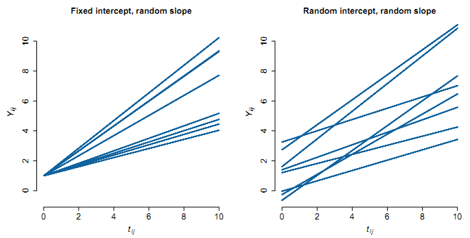
9.6.4 Linear mixed-effects model

For a continuous outcome $Y_{ij}$:

• Stage 1: Model for response given random effects:

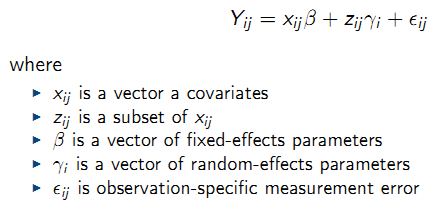
• Stage 2: Model for random effects:

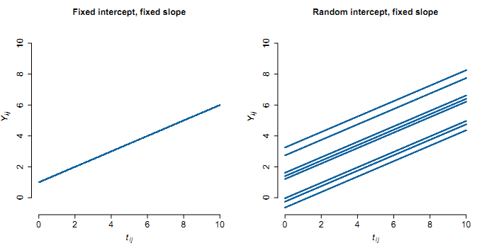
9.6.5 Choices for random effects

• Random intercepts:

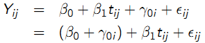
Fixed and Random Intercepts illustration:

• Random intercepts and slopes:

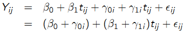
Random slope illustration:

9.6.6 Choices for random effects: G

G quantifies random variation in trajectories across subjects:

9.6.7 Basic models: Correlation

What is the correlation between measurements on the same subject?

9.6.7.1 Random intercepts model

Random intercept model correlation:

9.6.7.2 Random intercepts and slopes model

Random slope correlation:

9.6.8 Generalized linear mixed-effects models

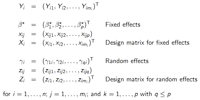
A GLMM is defined by random and systematic components:

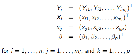
• Random: Conditional on $\gamma_{i}$ the outcomes $Y_{i} = (Y_{i1},...,Y_{im_{i}})^T$ are mutually independent and have an exponential family density.

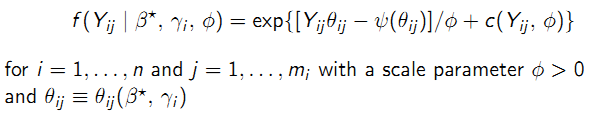
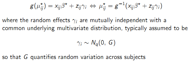
• Systematic: $\mu_{ij}^\star$ is modeled via a linear predictor containing fixed regression parameters $\beta^\star$ common to all individuals in the population and subject-specific random effects $\gamma_{i}$ with a known link function $g(.)$.

9.6.8.1 Likelihood-based estimation

Likelihood-based estimation of $\beta$: Requires specification of a complete probability distribution for the data

• Likelihood-based methods are designed for fixed effects, so integrate over the assumed distribution for the random effects:

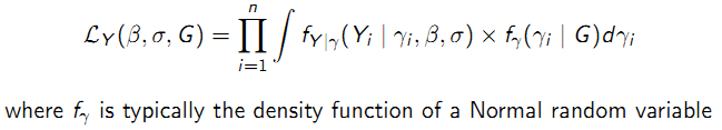
Two likelihood-based approaches to estimation using a GLMM:

• Conditional likelihood: Treat the random effects as if they were fixed parameters and eliminate them by conditioning on their sufficient statistics; does not require a specified distribution for $\gamma_{i}$.
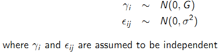
• Maximum likelihood: Treat the random effects as unobserved nuisance variables and integrate over their assumed distribution to obtain the marginal likelihood for $\beta$; typically assume $\gamma_{i}$~$N(0; G)$. (lmer and glmer in R package lme4)

9.6.9 Fixed effects vs. random effects

Fixed-effects approach provided by conditional likelihood estimation.

• Comparisons are made within individuals who act as their own control and differences are averaged across all individuals in the sample
• May eliminate potentially large sources of bias by controlling for all stable characteristics of the individuals under study (+)
• Variation across subjects is ignored, which may provide standard error estimates that are too big; conservative inference (-)
• Although controlled for by conditioning, cannot estimate coefficients for covariates that have no within-subject variation (-/+)

Random-effects approach provided by maximum likelihood estimation

• Comparisons are based on within- and between-subject contrasts
• Requires a specified distribution for subject-specific effects; correct specification is required for valid likelihood-based inference (-/+)
• Do not control for unmeasured characteristics because random effects are almost always assumed to be uncorrelated with covariates (-)
• Can estimate effects of within- and between-subject covariates (+)

9.6.9.1 Inference for $\beta$

Testing fixed effects in nested linear mixed-effects models:

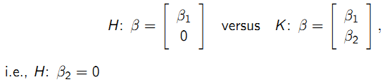
• Likelihood ratio test is valid if ML estimation is used
• Likelihood ratio test may not be valid with other estimation methods
• Wald test is generally valid

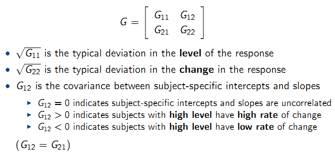
9.6.9.2 Inference for G

Testing whether a random intercept model is adequate:

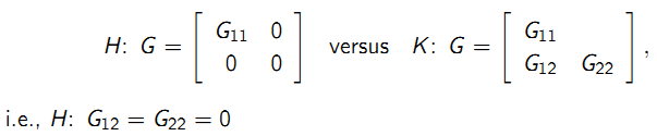
• Adequate covariance modeling is useful for the interpretation of the random variation in the data
• Over-parameterization of the covariance structure leads to inefficient estimation of fixed effects parameters $\beta$
• Covariance model choice determines the standard error estimates for $\hat{\beta}$; correct model is required for correct standard error estimates

9.6.9.3 Assumptions

Valid inference from a linear mixed-effects model relies on:

• Mean model: As with any regression model for an average outcome, need to correctly specify the functional form of $x_{ij}\beta$ (here also $z_{ij}\gamma_{i}$. – Included important covariates in the model – Correctly specified any transformations or interactions
• Covariance model: Correct covariance model (random-effects specification) is required for correct standard error estimates for $\hat{\beta}$.
• Normality: Normality of $\epsilon_{ij}$ and $\gamma_{i}$ is required for normal likelihood function to be the correct likelihood function for $Y_{ij}$.
• $n$ sufficiently large for asymptotic inference to be valid

These assumptions must be verified to evaluate any fitted model.

9.6.10 Summary

• Mixed-effects models assume that each subject has a regression model characterized by subject-specific parameters; a combination of fixed effects parameters common to all individuals in the population and random subject-specific perturbations
• Likelihood-based estimation and inference requires a complete parametric probability distribution for subject-specific random effects and error terms that must be verified for valid inference
• Estimates for the random effects are available

9.6.11 Issues

• Interpretation depends on outcomes and random-effects specification
• GLMM requires that any missing data are missing at random
• Issues arise with time-dependent exposures and covariance weighting

9.7 Mixed effect model formula in R

Mixed effect model may be fitted in R using the “lme4” package (Bates et al. 2024).

Source: Fitting Linear Mixed-Effects Models Using lme4

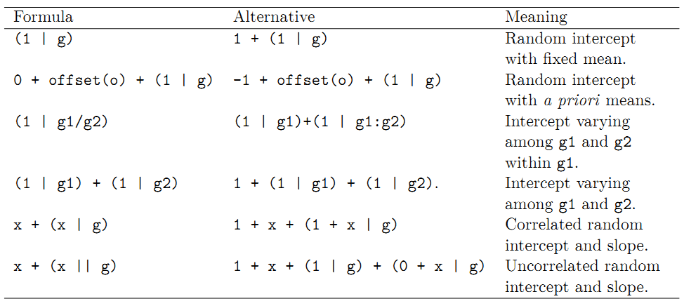
9.7.1 Formula

• resp ~ FEexpr + (REexpr1 | factor1) + (REexpr2 | factor2) + …, where FEexpr is an expression determining the columns of the ffxed-effects model matrix, X, and the random-effects terms, (REexpr1 | factor1) and (REexpr2 | factor2), determine both the random-effects model matrix, Z, and the structure of the relative covariance factor, $\Lambda_{\theta}$. In practice, the number of random-effects terms is typically low.
• Model formulas in R:

9.7.2 lme4 functions

Below are main functions of the package “lme4”.

9.7.3 Example Bangladesh data

Characterize waz among singletons and twins_triplets. Consider various specifications for the random effects structure:

• Random intercepts
• Random intercepts and slopes (for age)

Note: selection of a random effects structure should be guided by a priori knowledge and/or exploratory analysis, or specified as relevant to the scientific question of interest

9.7.3.1 GLMM with lme4

Package ‘lmerTest’ to get p-values.

#library(lme4)
#library(lmerTest) #for p-value 
waz.nona<-sh2 %>%
  filter(!is.na(waz))
r.in<-lmer(waz ~ age.m*cohort+ (1 | child.id), data=waz.nona)
summary(r.in)

## Linear mixed model fit by REML ['lmerMod']
## Formula: waz ~ age.m * cohort + (1 | child.id)
##    Data: waz.nona
## 
## REML criterion at convergence: 1344
## 
## Scaled residuals: 
##    Min     1Q Median     3Q    Max 
## -4.437 -0.565 -0.025  0.552  4.973 
## 
## Random effects:
##  Groups   Name        Variance Std.Dev.
##  child.id (Intercept) 0.721    0.849   
##  Residual             0.464    0.681   
## Number of obs: 573, groups:  child.id, 50
## 
## Fixed effects:
##                                      Estimate Std. Error t value
## (Intercept)                           0.09962    0.19176    0.52
## age.m                                -0.05498    0.00697   -7.89
## cohortHealthy Twins & Triplets       -3.47286    0.26529  -13.09
## age.m:cohortHealthy Twins & Triplets  0.06998    0.00969    7.23
## 
## Correlation of Fixed Effects:
##             (Intr) age.m  chHT&T
## age.m       -0.386              
## chrtHlthT&T -0.723  0.279       
## ag.m:chHT&T  0.277 -0.719 -0.354

r.s<-lmer(waz ~ age.m*cohort+ (age.m | child.id), data=waz.nona)
summary(r.s)

## Linear mixed model fit by REML ['lmerMod']
## Formula: waz ~ age.m * cohort + (age.m | child.id)
##    Data: waz.nona
## 
## REML criterion at convergence: 1239
## 
## Scaled residuals: 
##    Min     1Q Median     3Q    Max 
## -2.998 -0.510  0.007  0.525  4.531 
## 
## Random effects:
##  Groups   Name        Variance Std.Dev. Corr 
##  child.id (Intercept) 0.9505   0.975         
##           age.m       0.0126   0.112    -0.44
##  Residual             0.2939   0.542         
## Number of obs: 573, groups:  child.id, 50
## 
## Fixed effects:
##                                      Estimate Std. Error t value
## (Intercept)                            0.1027     0.2077    0.49
## age.m                                 -0.0549     0.0232   -2.37
## cohortHealthy Twins & Triplets        -3.6032     0.2913  -12.37
## age.m:cohortHealthy Twins & Triplets   0.0997     0.0332    3.01
## 
## Correlation of Fixed Effects:
##             (Intr) age.m  chHT&T
## age.m       -0.475              
## chrtHlthT&T -0.713  0.339       
## ag.m:chHT&T  0.332 -0.699 -0.479
## optimizer (nloptwrap) convergence code: 0 (OK)
## Model failed to converge with max|grad| = 0.00410411 (tol = 0.002, component 1)

There is a “moderate” correlation (-0.45) between random slopes and intercepts. If a strong correlation is observed, it is “over-parameterized” (too much of parameters”. In such cases, either intercept or slope is implemented as a random effect. We can also designate that intercepts and slopes are determined independently.

r.isi<-lmer(waz ~ age.m*cohort+ (1 | child.id)+(0+age.m | child.id), data=waz.nona)
summary(r.isi)

## Linear mixed model fit by REML ['lmerMod']
## Formula: waz ~ age.m * cohort + (1 | child.id) + (0 + age.m | child.id)
##    Data: waz.nona
## 
## REML criterion at convergence: 1248
## 
## Scaled residuals: 
##    Min     1Q Median     3Q    Max 
## -3.369 -0.515  0.002  0.532  4.608 
## 
## Random effects:
##  Groups     Name        Variance Std.Dev.
##  child.id   (Intercept) 0.8735   0.935   
##  child.id.1 age.m       0.0105   0.102   
##  Residual               0.2990   0.547   
## Number of obs: 573, groups:  child.id, 50
## 
## Fixed effects:
##                                      Estimate Std. Error t value
## (Intercept)                            0.1019     0.2003    0.51
## age.m                                 -0.0548     0.0213   -2.58
## cohortHealthy Twins & Triplets        -3.5907     0.2807  -12.79
## age.m:cohortHealthy Twins & Triplets   0.0972     0.0305    3.19
## 
## Correlation of Fixed Effects:
##             (Intr) age.m  chHT&T
## age.m       -0.081              
## chrtHlthT&T -0.714  0.058       
## ag.m:chHT&T  0.057 -0.698 -0.086

Comparing model with random intercept vs model with random intercept and slope. Random slope is significant.

# 
anova(r.in,r.s) 

## Data: waz.nona
## Models:
## r.in: waz ~ age.m * cohort + (1 | child.id)
## r.s: waz ~ age.m * cohort + (age.m | child.id)
##      npar  AIC  BIC logLik deviance Chisq Df Pr(>Chisq)    
## r.in    6 1337 1363   -662     1325                        
## r.s     8 1240 1275   -612     1224   100  2     <2e-16 ***
## ---
## Signif. codes:  0 '***' 0.001 '**' 0.01 '*' 0.05 '.' 0.1 ' ' 1

9.7.3.2 Get fixed effects and random effects

#fixed effects
fixef(r.s)

##                          (Intercept)                                age.m 
##                               0.1027                              -0.0549 
##       cohortHealthy Twins & Triplets age.m:cohortHealthy Twins & Triplets 
##                              -3.6032                               0.0997

#random effects
ranef(r.s)

## $child.id
##           (Intercept)    age.m
## Bgsng7018      0.1813 -0.01865
## Bgsng7035     -1.4131  0.02076
## Bgsng7052     -0.1744  0.02352
## Bgsng7063      0.8686 -0.04558
## Bgsng7071      1.0960 -0.01241
## Bgsng7082     -0.7357  0.04352
## Bgsng7090      0.2326 -0.00878
## Bgsng7096     -0.3517 -0.02508
## Bgsng7106      0.0299 -0.02547
## Bgsng7114     -0.5781  0.03357
## Bgsng7115      0.5440 -0.01088
## Bgsng7128     -1.1239  0.03577
## Bgsng7131     -0.3477 -0.04017
## Bgsng7142      0.5960 -0.06901
## Bgsng7149     -0.0745  0.02303
## Bgsng7150      0.6207 -0.01086
## Bgsng7155      0.2284 -0.07241
## Bgsng7173     -0.9953  0.02941
## Bgsng7177      0.4226 -0.07760
## Bgsng7178     -1.1764  0.07566
## Bgsng7192     -0.9135 -0.00481
## Bgsng7202      0.5255  0.00144
## Bgsng7204      0.1668  0.01788
## Bgsng8064      1.1785  0.08485
## Bgsng8169      1.1933  0.03230
## Bgtw1.T1       0.3700 -0.04224
## Bgtw1.T2       0.7327 -0.09384
## Bgtw10.T1      1.4475 -0.10310
## Bgtw10.T2      0.2469  0.02256
## Bgtw11.T1      0.2106 -0.09735
## Bgtw11.T2      0.6967 -0.06167
## Bgtw12.T1      0.1434 -0.19251
## Bgtw12.T2      0.6882 -0.17715
## Bgtw2.T1      -2.0567  0.02965
## Bgtw2.T2      -0.9605 -0.02606
## Bgtw3.T1       1.6332 -0.02464
## Bgtw3.T2       0.5931  0.02242
## Bgtw4.T1      -0.0146 -0.03925
## Bgtw4.T2       0.3240 -0.07395
## Bgtw4.T3       0.5405 -0.00948
## Bgtw5.T1      -2.0004  0.06607
## Bgtw5.T2       0.2573 -0.10866
## Bgtw6.T1      -0.4264  0.40051
## Bgtw6.T2      -1.2643  0.41722
## Bgtw7.T1       0.2326 -0.11179
## Bgtw7.T2      -0.6600 -0.06444
## Bgtw8.T1       1.5170  0.03427
## Bgtw8.T2       0.8968 -0.00457
## Bgtw9.T1      -1.3654  0.08765
## Bgtw9.T2      -1.7823  0.15036
## 
## with conditional variances for "child.id"

9.7.3.3 Visualization of results

Three types of plots:

9.7.3.3.1 Coefficients

Estimates:

#install.packages("glmmTMB")
#library(sjPlot)
#library(sjlabelled)
#library(sjmisc)
#library(ggplot2)
theme_set(theme_sjplot())
plot_model(r.s)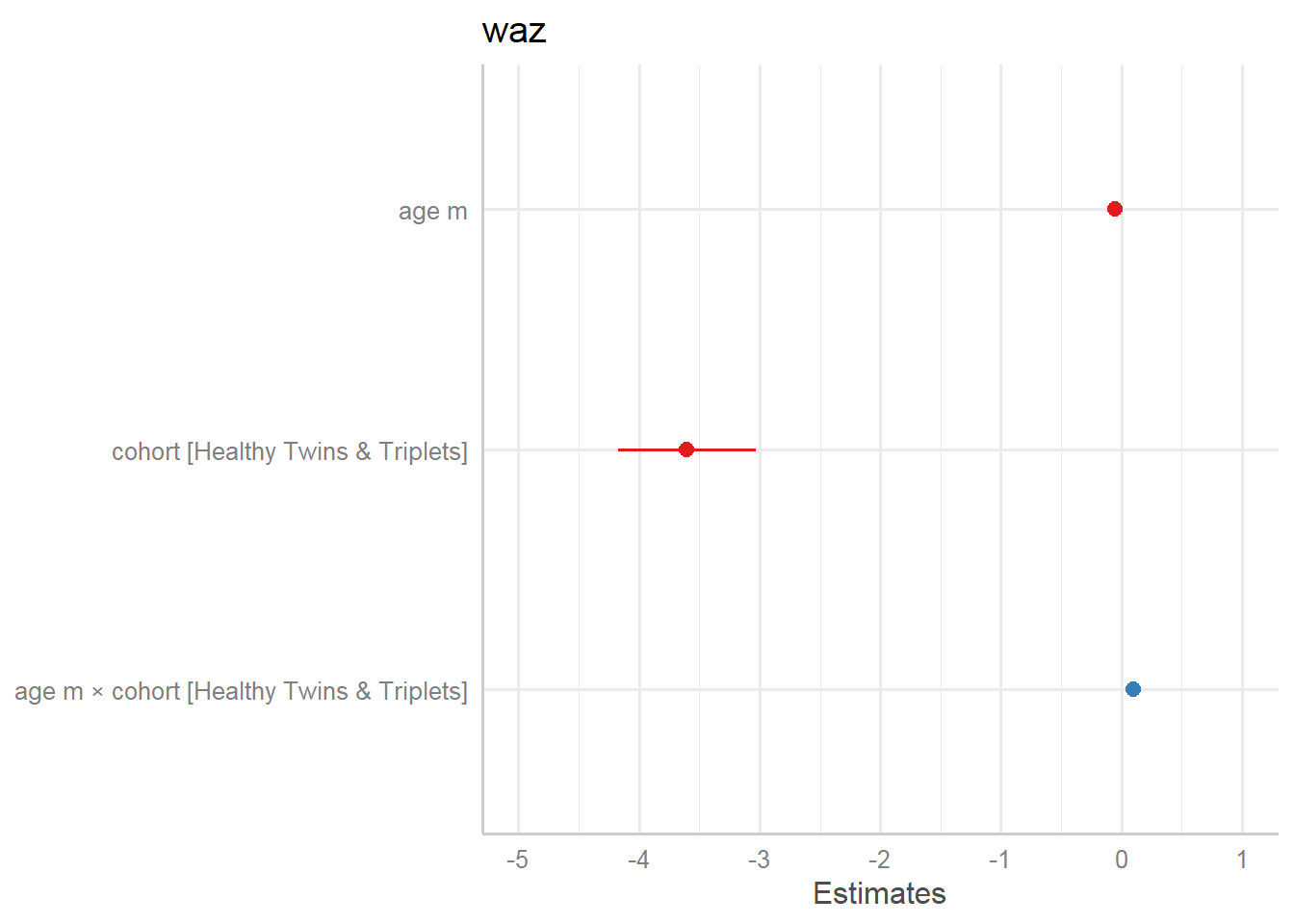

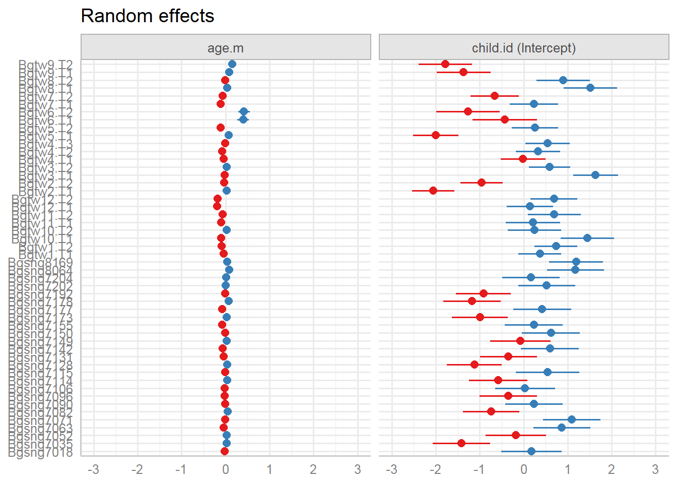
Random effects:

plot_model(r.s, type="re")

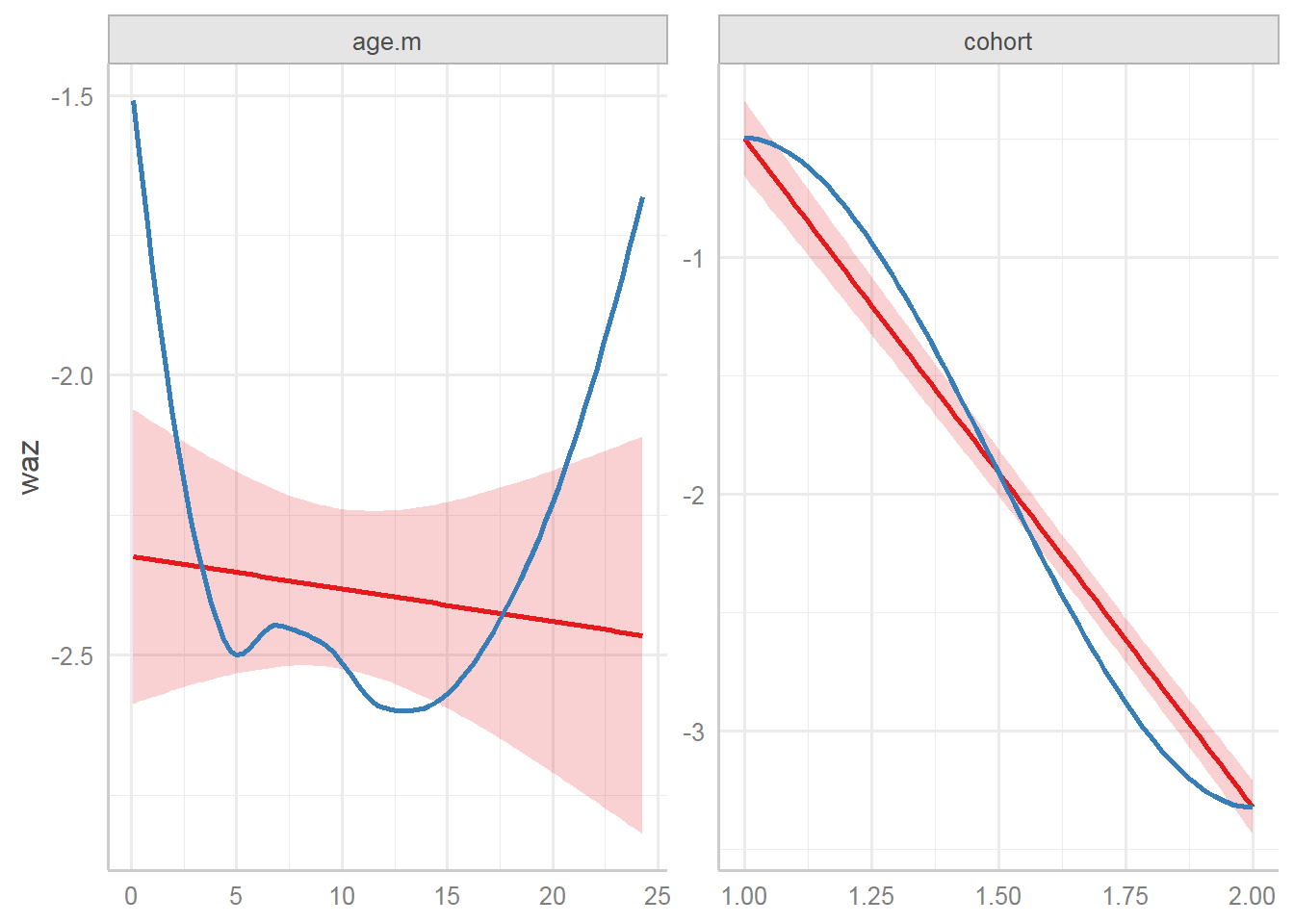
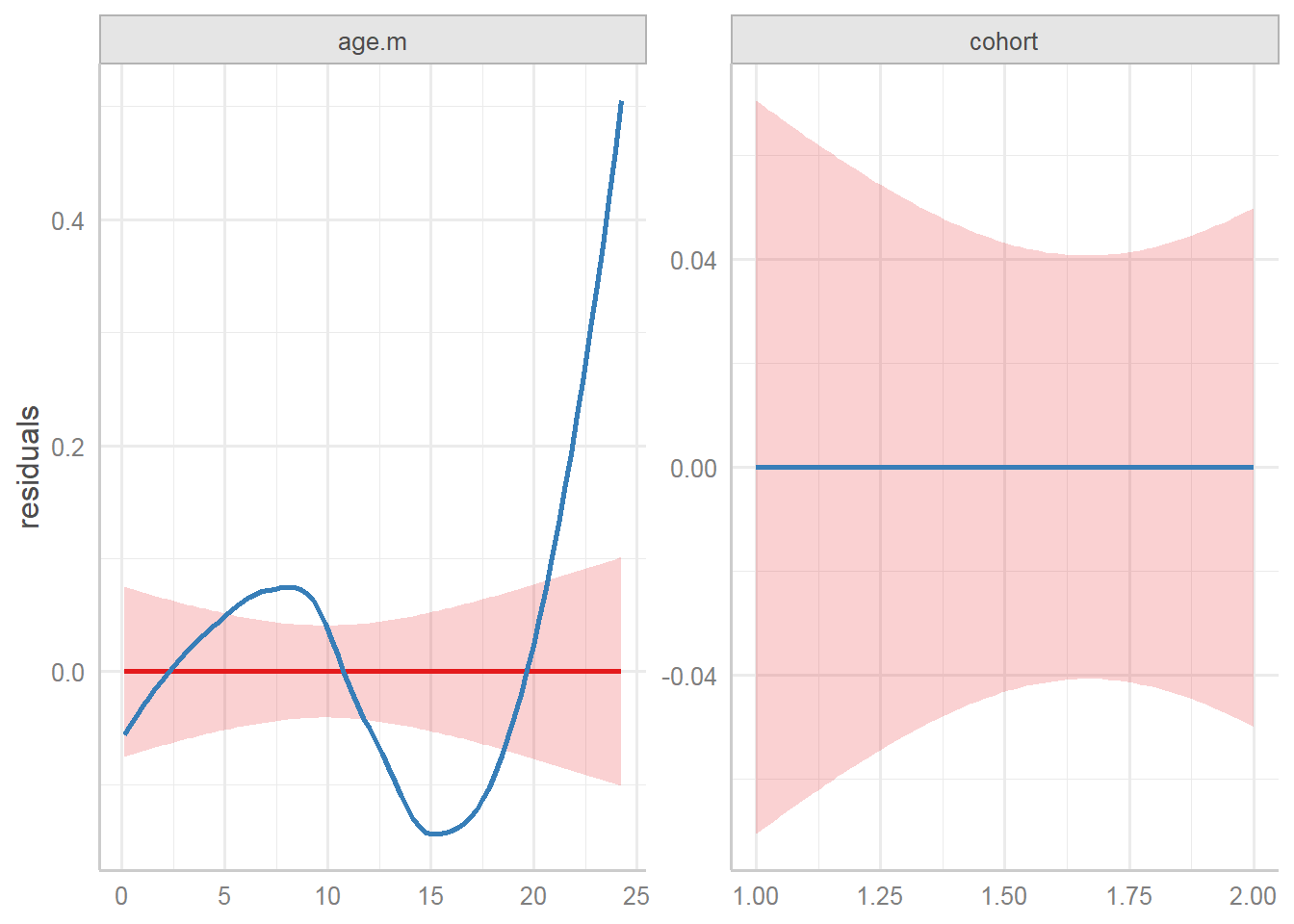
9.7.3.3.2 Marginal effects

Predicted values (marginal effects) for specific model terms:

plot_model(r.s, type="pred",show.data=T)

## $age.m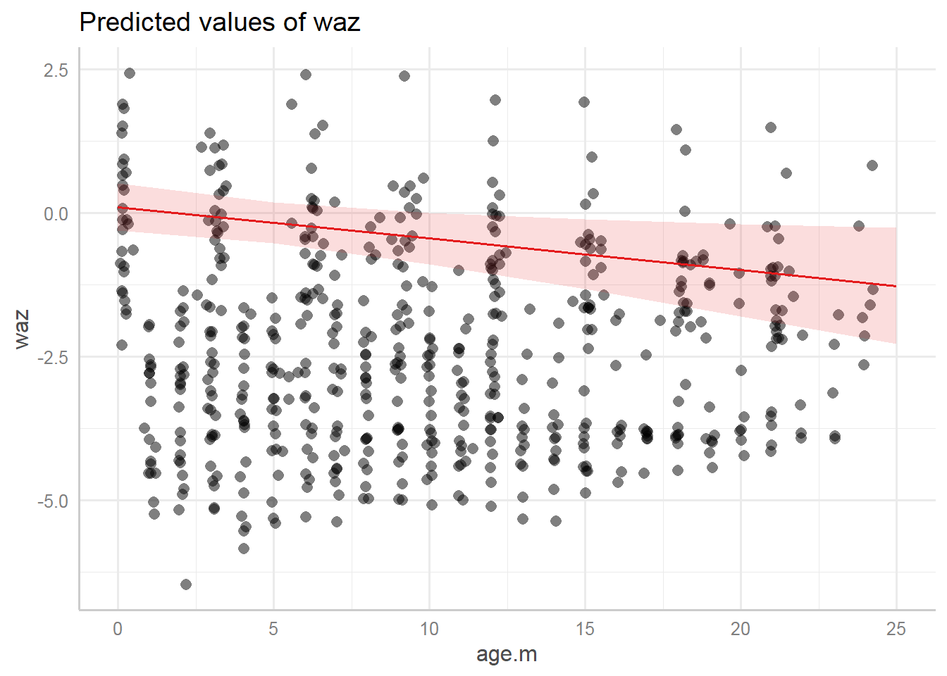

## 
## $cohort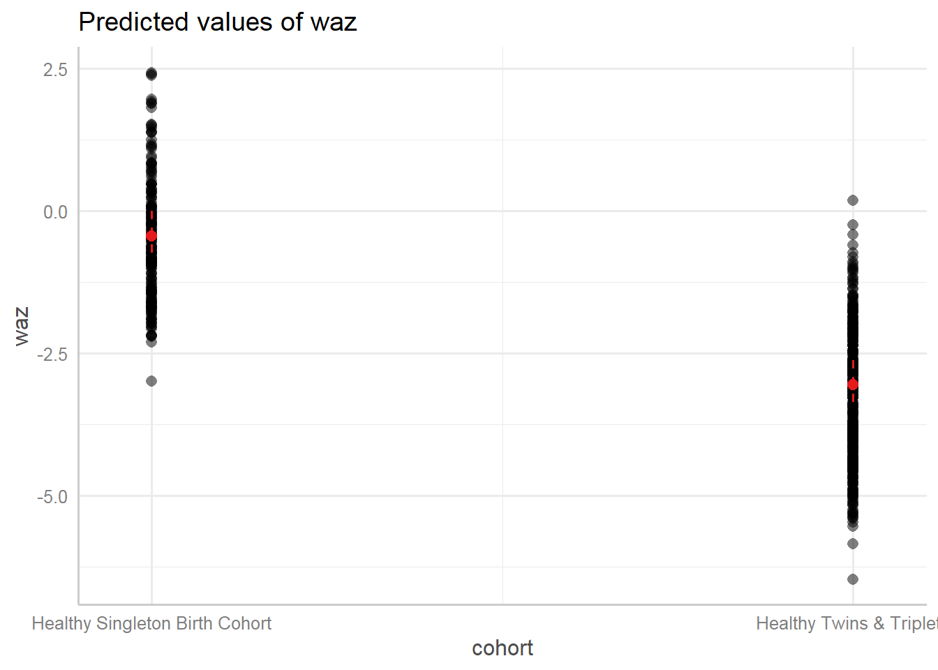

Marginal effects of interaction terms:

plot_model(r.s, type="int",show.data=T)

9.7.3.3.3 Model diagnostics

Slope of coefficients for each single predictor, against the response (linear relationship between each model term and response).

plot_model(r.s, type="slope")

Slope of coefficients for each single predictor, against the residuals (linear relationship between each model term and residuals).

plot_model(r.s, type="resid")

9.7.3.4 Summary of mixed model results

tab_model(r.s)

	waz
Predictors	Estimates	CI	p
(Intercept)	0.10	-0.31 – 0.51	0.621
age m	-0.05	-0.10 – -0.01	0.018
cohort [Healthy Twins & Triplets]	-3.60	-4.18 – -3.03	<0.001
age m × cohort [Healthy Twins & Triplets]	0.10	0.03 – 0.16	0.003
Random Effects
σ2	0.29
τ00 child.id	0.95
τ11 child.id.age.m	0.01
ρ01 child.id	-0.44
ICC	0.85
N child.id	50
Observations	573
Marginal R2 / Conditional R2	0.442 / 0.918

9.8 GEE or Mixed model

Summary of approaches for mixed models and GEE:

Two approaches have different targets for inferences and address subtly different questions about longitudinal change

• GEE: Marginal (population-average) Merely acknowledge the correlation among repeated measurements by robust variance estimation
• Mixed: Conditional (subject-specific) Provide an explanation for the source of correlation at different levels

Characteristics	Mixed model	GEE
Focus of interest	Variance component and regression coefficients	Regression coefficients
Parameter interpretation	Individual (subject, school, neighborhood) specific	Population average
Linear model (estimates equivalent)	Change in the mean outcome for a unit change in subject exposure, keeping the random effect (subject) fixed	Change in the mean outcome for a unit change in subject exposure across all of the subjects observed
Binary model (estimates not equivalent)	The log(OR) of an outcome for a unit change in subject exposure, keeping the subject fixed	The log(OR) of an outcome for a unit change in subject exposure across all of the subjects observed
Assumption	Correctly specified error distribution. Sensitive to different assumptions about variance and covariance structure, which are usually difficult to validate	Number of subjects should be sufficiently large for robust estimation of standard errors

9.9 Practice

Use the same example Bangladeshi children dataset as of this material, examine: - The change of haz over age, between cohort and gender - Visualize and interpret the results

Note: use GEE and/or GLMM where applicable.

9.10 Reference materials

This chapter has been adapted from several sources including:

9.10.1 Courses

• [SISCR Course 2016: “Introduction to Longitudinal Data Analysis”” by Benjamin French, PhD (University of Pennsylvania) and Colleen Sitlani, PhD (University of Washington)].

9.10.2 Online tutorials

• Fitting Linear Mixed-Effects Models Using lme4
• Visualizing (generalized) linear mixed effects models with ggplot #rstats #lme4; Part 2.
• INTRODUCTION TO GENERALIZED LINEAR MIXED MODELS.
• GENERALIZED ESTIMATING EQUATIONS (GEE)
• To GEE or not to GEE.

9.10.3 Books, other resources

• APPLIED LONGITUDINAL DATA ANALYSIS.
• Linear Mixed-Effects Models Using R.

References

Bates, Douglas, Martin Maechler, Ben Bolker, and Steven Walker. 2024. Lme4: Linear Mixed-Effects Models Using Eigen and S4. https://github.com/lme4/lme4/.

Gałecki, Andrzej, and Tomasz Burzykowski. 2013. Linear Mixed-Effects Models Using r. Springer New York. https://doi.org/10.1007/978-1-4614-3900-4.

Højsgaard, Søren, Ulrich Halekoh, and Jun Yan. 2024. Geepack: Generalized Estimating Equation Package. https://CRAN.R-project.org/package=geepack.