Chapter 7 Logistic Regression with R

Phuong Thi Minh Chu, Msc and Nhan Thi Ho, MD, PhD

7.1 Introduction

7.1.1 Data types

Discrete and continuous data types:

• Discrete data (categorical data) is counted. Discrete data can only take certain values (individually separated and distinct). Example: The number of patients in a hospital (we can’t have half patient!), Yes/No, Male/Female,… There are two types of categorical variables: A nominal variable has no intrinsic ordering to its categories. Example: Male/Female An ordinal variable has a clear ordering. Example: clothes sizes small/medium/big
• Continuous data is measured. Continuous data can take any value (within a range). Example: Height, Weight, The length of a leaf,…

7.1.2 Classification and Regression

• Classification is the task of predicting a discrete class label (discrete output type).
• Regression is the task of predicting a continuous quantity (continuous output type).

Example:

Output	Data	Task
Disease yes or no	Discrete	Classification
Benign or malignant tumor	Discrete	Classification
Blood IgG level	Continuous	Regression
Body Mass Index (BMI)	Continuous	Regression

7.1.3 Logistic Regression and Linear Regression

If Linear Regression serves to predict continuous variables, Logistic Regression is used for binary classification.

Example: The diabetes data: predict outcome diabetes using other variables such as BMI, skin thickness, blood glucose,…

First, take a look at the dataset and examine relationship between bmi and outcome by linear regression.

# Load example data 
data<-read.csv("https://raw.githubusercontent.com/plotly/datasets/master/diabetes.csv")
colnames(data)<-tolower(colnames(data))
str(data)

## 'data.frame':    768 obs. of  9 variables:
##  $ pregnancies             : int  6 1 8 1 0 5 3 10 2 8 ...
##  $ glucose                 : int  148 85 183 89 137 116 78 115 197 125 ...
##  $ bloodpressure           : int  72 66 64 66 40 74 50 0 70 96 ...
##  $ skinthickness           : int  35 29 0 23 35 0 32 0 45 0 ...
##  $ insulin                 : int  0 0 0 94 168 0 88 0 543 0 ...
##  $ bmi                     : num  33.6 26.6 23.3 28.1 43.1 25.6 31 35.3 30.5 0 ...
##  $ diabetespedigreefunction: num  0.627 0.351 0.672 0.167 2.288 ...
##  $ age                     : int  50 31 32 21 33 30 26 29 53 54 ...
##  $ outcome                 : int  1 0 1 0 1 0 1 0 1 1 ...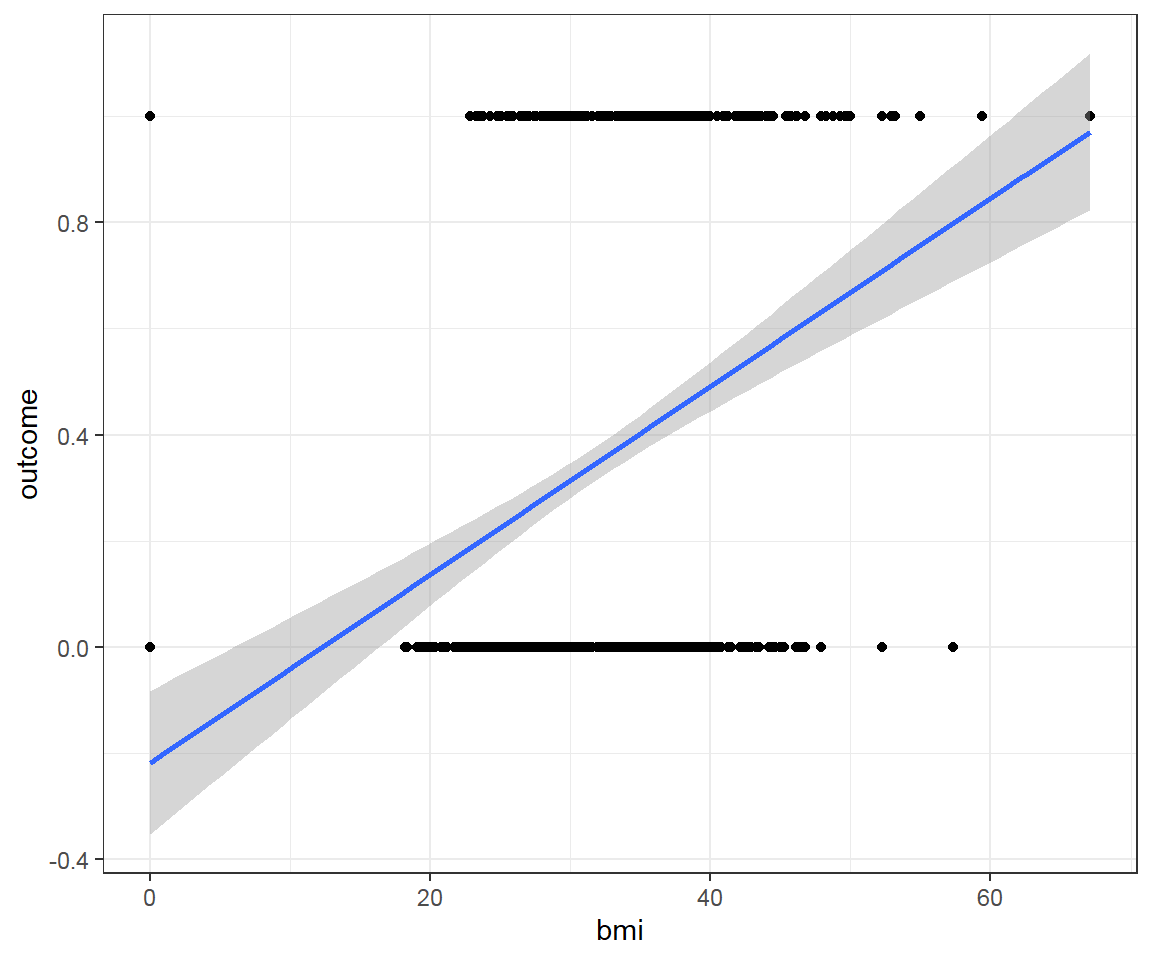

ggplot(data, aes(bmi, outcome))+
  geom_point()+
  geom_smooth(method='lm', formula= y~x)

Where:

• 0 means there is no outcome (diabetes), 1 means there is the outcome (diabetes)

• What we try to predict is the likelihood of having the outcome (diabetes)

• This may be represented as following:

  • y-axis/target being the Probability of having the outcome (diabetes)

    • 0 = 0% of having the outcome (diabetes)
    • 1 = 100% of having the outcome (diabetes)

  • x-axis = the bmi values

• This is a bad fit line, because it cannot capture the pattern of data. It does not go through most of data points.

• Furthermore:

  • When bmi decreases, we predict negative probability!
  • With higher bmi, we even predict probability larger than 1!
  • The predictions are not sensible as the probability must fall between 0 and 1

Solution: Transform a Linear Regression line to a Logistic Regression curve, which can only go between 0 and 1.

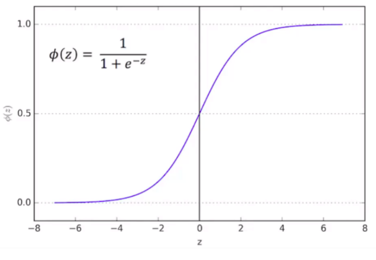
Logistic function is one type of Sigmoid function:

• Mathematical form: $\phi(z) = \frac{1}{1+e^{-z}}$
• Graphical form: S-curve
• Note : it doesn’t matter what value of Z we put into the logistic function, you will always get a value of 0 and 1, which just meets the requirements that we need.

Therefore, Logistic Regression function results in a probability from 0 to 1.

Comparison:

Differences	Linear Regression	Logistic Regression
Function	$y=a_o+a_1x+ε$ where, $a_o$ and $a_1$ are the coefficients and ε is the error term	$log[\frac{y}{1−y}]=b_o+b_1x_1+b_2x_2+b_3x_3+...+b_nx_n$
Label data	Continuous dependent variable (Continuous data)	Categorical dependent variable (Discrete data)
Problem	Regression problem	Classification problems
Model	Find the best fit line (straight line), by which we can easily predict the output	Find the S-curve by which we can classify the samples
Problem’s output	Continuous value, such as price, age, etc	Categorical value such as 0 or 1, Yes or No, etc
Collinearity	There may be collinearity between the independent variables	There should not be collinearity between the independent variable

7.2 Logistic regression

7.2.1 Statistical concept overview

Logistic Regression can be used for both traditional statistics and machine learning. Logistic Regression is a specific type of Generalized Linear Model (GLM). GLM are a generalization of the concepts and abilities of regular Linear Models. Therefore, if ones are familiar with Linear Models, then ones may understand Logistic Regression.

A Logistic Regression will model the chance of an outcome based on individual characteristics. Because chance is a ratio, what will be actually modeled is the logarithm of the chance given by:

$log[\frac{y}{1−y}]=b_o+b_1x_1+b_2x_2+b_3x_3+...+b_nx_n$ where:

• $y$ indicates the probability of an event
• $b_i$ are the regression coefficients associated with the reference group and the $x_i$ explanatory variables.
• The reference group, represented by $b_o$, is constituted by those individuals presenting the reference level of each and every variable $x_{1...n}$.

7.2.1.1 Coefficients

In terms of the coefficients, Logistic Regression is similar as Linear models except the coefficients are in terms of the log(odds).

Example: Given a person profile of BMI, blood glucose, blood pressure, our aim is to build a model that predict the probability of that person getting diabetes.

This is part of the coefficients from logistic regression model fitted with glm (R Core Team 2024b):

# Load example data 
data<-read.csv("https://raw.githubusercontent.com/plotly/datasets/master/diabetes.csv")
colnames(data)<-tolower(colnames(data))
data$outcome<-as.factor(data$outcome) 
# Multivariate model
logistic <- glm(outcome ~ bmi + glucose + bloodpressure,data=data,family="binomial")
summary(logistic)$coefficients

##                   Estimate  Std. Error    z value     Pr(>|z|)
## (Intercept)   -7.182306362 0.635461655 -11.302502 1.275325e-29
## bmi            0.079792571 0.013565206   5.882149 4.049725e-09
## glucose        0.035746292 0.003328357  10.739920 6.610136e-27
## bloodpressure -0.007420144 0.004861549  -1.526292 1.269371e-01

• The Intercept gives the mean level of the response variable when all other variables are 0. The estimated intercept is -7.1823064, the standard error of the estimated intercept is 0.6354617. The z value is the estimated intercept divided by the standard error. In other words, it’s the number of standard deviations the estimated intercept is away from 0 on a standard normal curve.
• Each one-unit change in bmi will increase the log (odds) of getting the outcome (diabetes) by 0.0797926, and its p value indicates that it is significant in determining the outcome.

7.2.1.2 Maximum Likelihood

How to select the correct sigmoid function that best fits the data?

This is the main question for Logistic Regression. The answer is by using maximum likelihood. In other words, which sigmoid function would generate the observed data with the highest probability?

Logistic Regression models are fitted using the method of maximum likelihood - i.e. the parameter estimates are those values which maximize the likelihood of the data which have been observed.

Example: Given a problem of the number of cigarettes which a patient smoke per month and the outcome of having lung cancer or not.

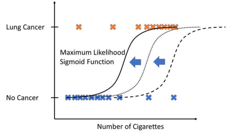
To calculate the likelihood for a given set of training data, you simply calculate the likelihood for a single training date and repeat this procedure for all training dates. Finally, you multiply those to get the likelihood for the whole set of training data.

Now, you proceed this same likelihood computation for different sigmoid functions (shifting the sigmoid function a little bit). From all computations, you take the sigmoid function that has “maximum likelihood” that means which would produce the training data with maximal probability.

7.2.1.3 R-squared and p-value

With maximum likelihood, we have the best fit line. However, how do we know if that best fit line is useful?

We use $R^2$ and associated p-value!

• R squared: Even though everyone agrees on how to calculate $R^2$ and associated p-value for Linear Models, there is no consensus on how to calculate $R^2$ for Logistic Regression. There are more than 10 different ways to do it! One of the most common method is “McFadden’s Pseudo $R^2$”. This method is very similar to the method in Linear Model. McFadden’s R squared measure is defined as: $R^2_{McFadden} = 1-\frac{log(L_c)}{log(L_{null})}$

where Lc denotes the (maximized) likelihood value from the current fitted model, and Lnull denotes the corresponding value but for the null model - the model with only an intercept and no covariates.

The log-likelihood R2 values go from 0, for poor models, to 1, for good models.

• p-values: Calculating the p-value to determine if R2 value is statistically significant.

7.2.2 Univariable and multivariable models

In Logistic Regression the outcome or dependent variable is binary. The predictor or independent variable is one with univariable model and more than one with multivariable model. In reality, most outcomes have many predictors. Hence, multivariable Logistic Regression mimics reality.

7.2.3 Model building and selection

7.2.3.1 Main steps

Main steps of building Logistic Regression (logit) models:

• Import data
• Clean data and check for class bias
• Create training and test samples
• Compute information value to find out important variables
• Build logit models
• Predict on test data
• Do model evaluation

7.2.3.2 Building model in R

Example: We use the same example diabetes dataset above. Our aim is to build a model so that predict the probability of having the outcome (diabetes) if profile is given.

7.2.3.2.1 Import data

Import the dataset and take a look at the data’s structure by using function str() and summarize all variables in the dataset by outcome and overall:

# Load example data 
data<-read.csv("https://raw.githubusercontent.com/plotly/datasets/master/diabetes.csv")
colnames(data)<-tolower(colnames(data))
str(data)

## 'data.frame':    768 obs. of  9 variables:
##  $ pregnancies             : int  6 1 8 1 0 5 3 10 2 8 ...
##  $ glucose                 : int  148 85 183 89 137 116 78 115 197 125 ...
##  $ bloodpressure           : int  72 66 64 66 40 74 50 0 70 96 ...
##  $ skinthickness           : int  35 29 0 23 35 0 32 0 45 0 ...
##  $ insulin                 : int  0 0 0 94 168 0 88 0 543 0 ...
##  $ bmi                     : num  33.6 26.6 23.3 28.1 43.1 25.6 31 35.3 30.5 0 ...
##  $ diabetespedigreefunction: num  0.627 0.351 0.672 0.167 2.288 ...
##  $ age                     : int  50 31 32 21 33 30 26 29 53 54 ...
##  $ outcome                 : int  1 0 1 0 1 0 1 0 1 1 ...

#convert outcome to factor
data$outcome<-as.factor(data$outcome) 

#summary of all variables in the dataset
my_controls <- tableby.control(
  test = T,
  total = T,
  numeric.stats = c("meansd", "medianq1q3","meanCI","range","Nmiss2"),
  cat.stats = c("countpct", "Nmiss2"),
  stats.labels = list(
    meansd = "Mean (SD)",
    medianq1q3 = "Median (Q1, Q3)",
    range = "Min - Max",
    Nmiss2 = "Missing",
    meanCI = "Mean (95%CI)"
  )
)
prevar<-colnames(data)[!colnames(data) %in% "outcome"]
mylabels <-as.list(prevar)
names(mylabels)<-prevar
tab <- tableby(as.formula(paste("outcome",paste(prevar,collapse="+"),sep="~")),
                data = data,
                control = my_controls)
kable(summary(tab,labelTranslations = mylabels, text=TRUE))

	0 (N=500)	1 (N=268)	Total (N=768)	p value
pregnancies				< 0.001
- Mean (SD)	3.298 (3.017)	4.866 (3.741)	3.845 (3.370)
- Median (Q1, Q3)	2.000 (1.000, 5.000)	4.000 (1.750, 8.000)	3.000 (1.000, 6.000)
- Mean (95%CI)	3.298 (3.033, 3.563)	4.866 (4.416, 5.316)	3.845 (3.606, 4.084)
- Min - Max	0.000 - 13.000	0.000 - 17.000	0.000 - 17.000
- Missing	0	0	0
glucose				< 0.001
- Mean (SD)	109.980 (26.141)	141.257 (31.940)	120.895 (31.973)
- Median (Q1, Q3)	107.000 (93.000, 125.000)	140.000 (119.000, 167.000)	117.000 (99.000, 140.250)
- Mean (95%CI)	109.980 (107.683, 112.277)	141.257 (137.416, 145.099)	120.895 (118.630, 123.159)
- Min - Max	0.000 - 197.000	0.000 - 199.000	0.000 - 199.000
- Missing	0	0	0
bloodpressure				0.072
- Mean (SD)	68.184 (18.063)	70.825 (21.492)	69.105 (19.356)
- Median (Q1, Q3)	70.000 (62.000, 78.000)	74.000 (66.000, 82.000)	72.000 (62.000, 80.000)
- Mean (95%CI)	68.184 (66.597, 69.771)	70.825 (68.240, 73.409)	69.105 (67.734, 70.477)
- Min - Max	0.000 - 122.000	0.000 - 114.000	0.000 - 122.000
- Missing	0	0	0
skinthickness				0.038
- Mean (SD)	19.664 (14.890)	22.164 (17.680)	20.536 (15.952)
- Median (Q1, Q3)	21.000 (0.000, 31.000)	27.000 (0.000, 36.000)	23.000 (0.000, 32.000)
- Mean (95%CI)	19.664 (18.356, 20.972)	22.164 (20.038, 24.291)	20.536 (19.406, 21.666)
- Min - Max	0.000 - 60.000	0.000 - 99.000	0.000 - 99.000
- Missing	0	0	0
insulin				< 0.001
- Mean (SD)	68.792 (98.865)	100.336 (138.689)	79.799 (115.244)
- Median (Q1, Q3)	39.000 (0.000, 105.000)	0.000 (0.000, 167.250)	30.500 (0.000, 127.250)
- Mean (95%CI)	68.792 (60.105, 77.479)	100.336 (83.656, 117.016)	79.799 (71.636, 87.963)
- Min - Max	0.000 - 744.000	0.000 - 846.000	0.000 - 846.000
- Missing	0	0	0
bmi				< 0.001
- Mean (SD)	30.304 (7.690)	35.143 (7.263)	31.993 (7.884)
- Median (Q1, Q3)	30.050 (25.400, 35.300)	34.250 (30.800, 38.775)	32.000 (27.300, 36.600)
- Mean (95%CI)	30.304 (29.629, 30.980)	35.143 (34.269, 36.016)	31.993 (31.434, 32.551)
- Min - Max	0.000 - 57.300	0.000 - 67.100	0.000 - 67.100
- Missing	0	0	0
diabetespedigreefunction				< 0.001
- Mean (SD)	0.430 (0.299)	0.550 (0.372)	0.472 (0.331)
- Median (Q1, Q3)	0.336 (0.230, 0.562)	0.449 (0.263, 0.728)	0.372 (0.244, 0.626)
- Mean (95%CI)	0.430 (0.403, 0.456)	0.550 (0.506, 0.595)	0.472 (0.448, 0.495)
- Min - Max	0.078 - 2.329	0.088 - 2.420	0.078 - 2.420
- Missing	0	0	0
age				< 0.001
- Mean (SD)	31.190 (11.668)	37.067 (10.968)	33.241 (11.760)
- Median (Q1, Q3)	27.000 (23.000, 37.000)	36.000 (28.000, 44.000)	29.000 (24.000, 41.000)
- Mean (95%CI)	31.190 (30.165, 32.215)	37.067 (35.748, 38.386)	33.241 (32.408, 34.074)
- Min - Max	21.000 - 81.000	21.000 - 70.000	21.000 - 81.000
- Missing	0	0	0

We can notice that there are a greater number of outcome =0 (no diabetes) than outcome =1 (diabetes). From the summary table, we can see the variables showing unbalance between outcome =0 (no diabetes) and outcome =1 (diabetes).

7.2.3.2.2 Build Logistic Regression model in R

Note: For simplicity, we will build our model with all the data (no train-test splitting). For predictive modeling, we will need to do develop model on training data and validate model on test data.

The glm() procedure with family="binomial" will build the Logistic Regression model on the given formula.

# Univariate model
fitu <- glm(outcome ~ bmi,data=data,family="binomial")

# Multivariate model
fitm <- glm(outcome ~ bmi + glucose + bloodpressure,data=data,family="binomial")

• data=data data frame named data
• family="binomial" for Logistic Regression model
• outcome is the column which contains the response variable outcome
• ~ help us select the predictors:
  • . means chose all the data that we have.
  • If we want to chose specific variables as predictors, we can replace . with the combination of your interested variables. For example, ~ bmi for chosing only bmi; ~ bmi + glucose + bloodpressure for chosing bmi, glucose, bloodpressure.
  • You can even exclude the predictor. For example, you write ~. - glucose to unselect variable glucose and end up with fitm <- glm(outcome ~. - glucose, data=data, family="binomial")

7.2.3.2.3 Interpretation of results

summary(fitm)

## 
## Call:
## glm(formula = outcome ~ bmi + glucose + bloodpressure, family = "binomial", 
##     data = data)
## 
## Coefficients:
##                Estimate Std. Error z value Pr(>|z|)    
## (Intercept)   -7.182306   0.635462 -11.303  < 2e-16 ***
## bmi            0.079793   0.013565   5.882 4.05e-09 ***
## glucose        0.035746   0.003328  10.740  < 2e-16 ***
## bloodpressure -0.007420   0.004862  -1.526    0.127    
## ---
## Signif. codes:  0 '***' 0.001 '**' 0.01 '*' 0.05 '.' 0.1 ' ' 1
## 
## (Dispersion parameter for binomial family taken to be 1)
## 
##     Null deviance: 993.48  on 767  degrees of freedom
## Residual deviance: 769.07  on 764  degrees of freedom
## AIC: 777.07
## 
## Number of Fisher Scoring iterations: 4

• Deviance Residuals: Summary of the distribution of the deviance residuals. Deviance residuals measure how well the observations fit the model. The closer a residual to 0 the better the fit of the observation.

• Coefficients:

  • In general, the Intercept gives the mean level of the response variable when all other variables are 0. The estimated intercept is -7.1823064, the standard error of the estimated intercept is 0.6354617, and the z value is the estimated intercept devided by the standard error.

  • Each one-unit change in bmi will increase the log (odds) of getting outcome by 0.0797926, and its p value indicates that it is significant in determining the outcome.

  • Each unit increase in glucose increases the log odds of getting outcome by 0.0357463 and p value indicates that it is significant in determining the outcome.

  • bloodpressure is not significant in determining the outcome.

• Deviance: Null deviance is the value when you only have intercept in your equation with no variables and Residual deviance is the value when you are taking all the variables into account. It makes sense to consider the model good if that difference is big enough. Generally, the degrees of freedom reported on the Null deviance are always higher than the degrees of freedom reported on the Residual deviance.

The difference between Null deviance and Residual deviance tells us that our model is a good fit. Greater the difference better the model.

• Akaike Information Criterion (AIC): The Akaike Information Criterion (AIC) provides a method for assessing the quality of your model through comparison of related models. It’s based on the Deviance, but penalizes you for making the model more complicated. Much like adjusted R-squared, it’s intent is to prevent you from including irrelevant predictors.

However, unlike adjusted R-squared, the number itself is not meaningful. If you have more than one similar candidate models (where all of the variables of the simpler model occur in the more complex models), then you should select the model that has the smallest AIC.

So it’s useful for comparing models, but isn’t interpretable on its own.

• Fisher Scoring: Fisher’s scoring algorithm is a derivative of Newton’s method for solving maximum likelihood problems numerically. This tells you that the model successfully performs the fit with 4 iterations.

7.2.3.2.4 Making prediction

Let’s predict if a person has a profile of bmi=29, glucose=148, bloodpressure=96, what is the probability of that person getting outcome=1.

x <- data.frame(bmi=29, glucose=148, bloodpressure=96)
p<- predict(fitm,x, type="response")
p

##         1 
## 0.4279538

We see that there is 0.4279538 chance that she will get outcome=1.

7.2.4 Model evaluation

7.2.4.1 Confusion Matrix

It is good to visualize classification results using the confusion matrix:

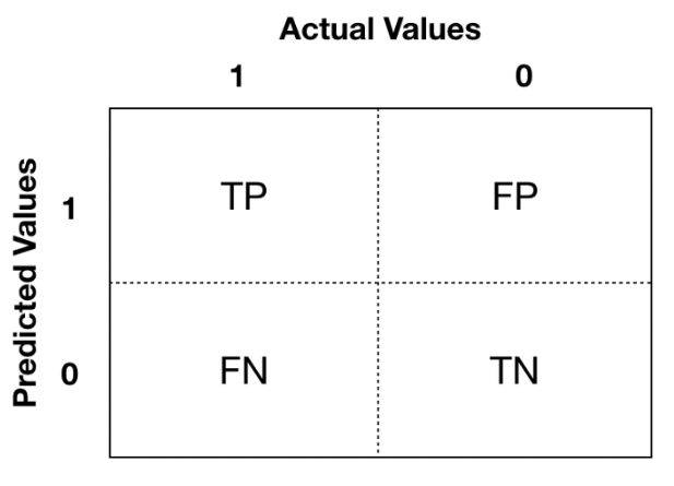
The Positive/Negative label refers to the predicted outcome of an experiment, while the True/False refers to the actual outcome.

• Type 1 error corresponds to a False Positive.
• Type 2 error corresponds to a False Negative.

You focus more on which aspect you want to improve base on your specific problems. Example: if you build a model to identify if a breast cancer is benign or malignant -> prefer Type 2 error to Type 1 error because you do not want to miss malignant cases.

7.2.4.2 Confusion Metrics

From the confusion matrix, different metrics can be measured for the validity of the model:

• Accuracy (all correct / all): ACC=(TP+TN)/(TP+TN+FP+FN)

• Misclassification or Error rate (all incorrect / all): Misclassification=(FP+FN)/(TP+TN+FP+FN)

• Precision or Positive predictive value (PPV) (true positives / predicted positives): Precision=TP/(TP+FP)

• Sensitivity or Recall or true positive rate (true positives / all actual positives): Sensitivity refers to the test’s ability to correctly detect ill patients who do have the condition. Sensitivity=TP/(TP+FN)

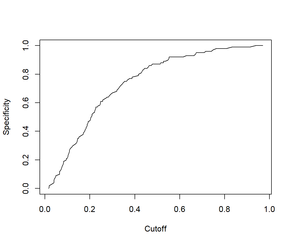
• Specificity (true negatives / all actual negatives): A positive result in a test with high specificity is useful for ruling in disease. The test rarely gives positive results in healthy patients. A positive result signifies a high probability of the presence of disease. Specificity=TN/(TN+FP)

The accuracy score might not be the best metrics to use for a classification problem, especially if you deal with the unbalanced dataset.

7.2.4.3 F1-score

It is difficult to compare two models with low precision and high recall or vice versa. So to make them comparable, we use F1-score. F1-score helps to measure Recall and Precision at the same time.

$F_1=2\frac{Recall.Precision}{(Recall+Precision)}$

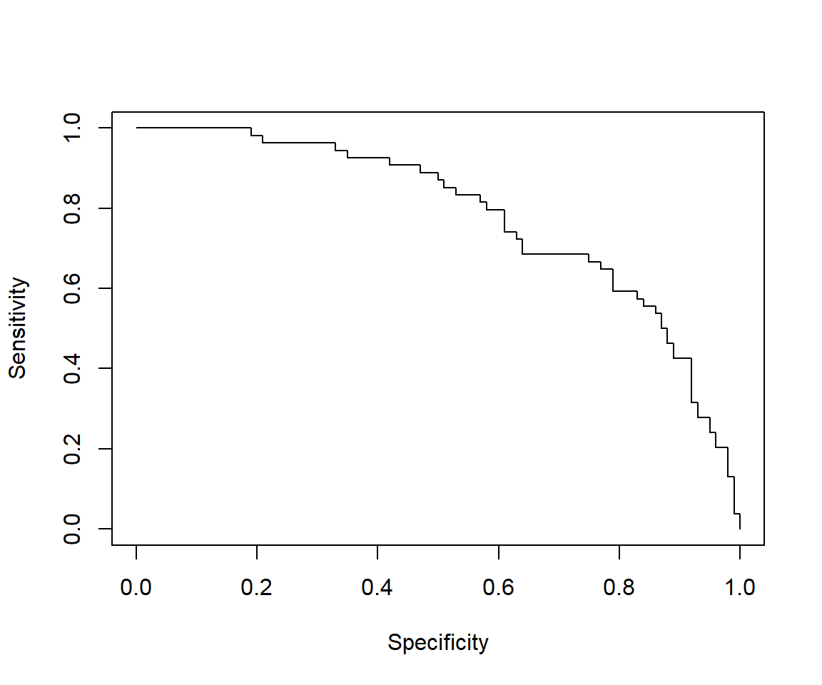
7.2.4.4 Receiver Operating Characteristics Curve (ROC)

Receiver Operating Characteristics Curve (ROC) traces the percentage of TP accurately predicted by a given model as the prediction probability cutoff is lowered from 1 to 0. We will mostly use the R package “ROCR” for evaluation of model performance (Tobias Sing et al. 2020).

library(ROCR)
predicted <- predict(fitm, type="response")  

# Create a prediction object
pred <- prediction(predicted, data$outcome)

# Create a performance object
perf <- performance(pred,"tpr","fpr")
# ROC curve
plot(perf, main="Receiver Operating Characteristics Curve (ROC)")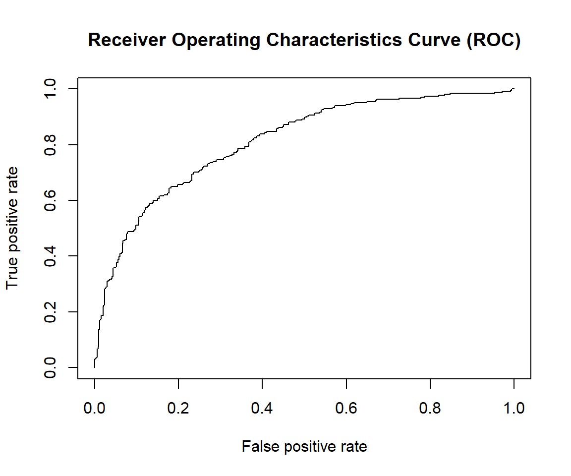

For a good model:

• As the cutoff is lowered, it should mark more of actual label 1 as positives and lesser of actual label 0 as label 1.

• The curve should rise steeply, indicating that the TPR (Y-Axis)(or Sensitivity) increases faster than the FPR (X-Axis)(or Specificity) as the cutoff score decreases.

• Greater the area under the ROC curve (AUC), better the predictive ability of the model.

7.2.4.5 Some other performance measures

# Other performance measures
# Sensitivity by cutoff
perf <- performance(pred,"sens","cutoff")
plot(perf)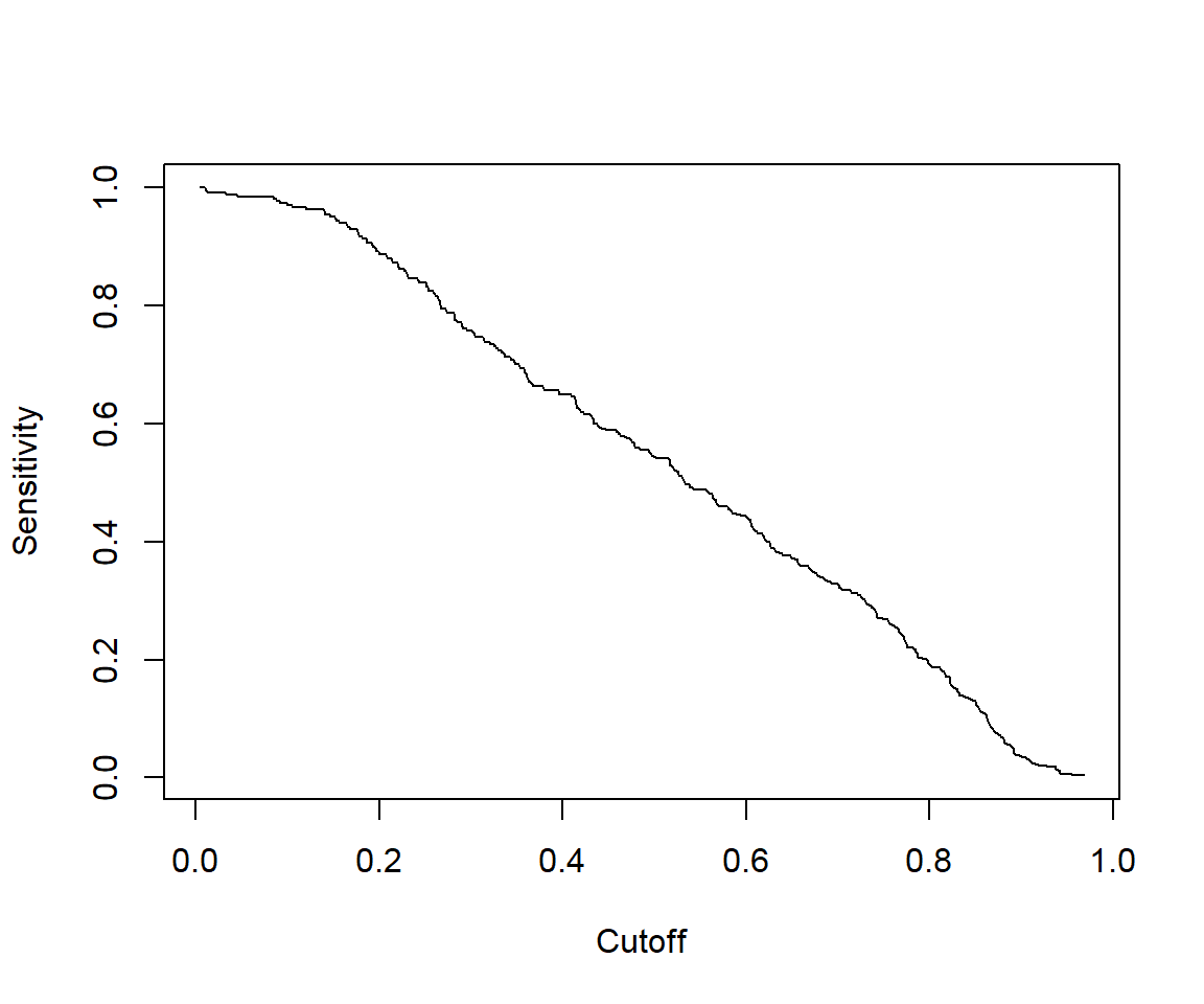

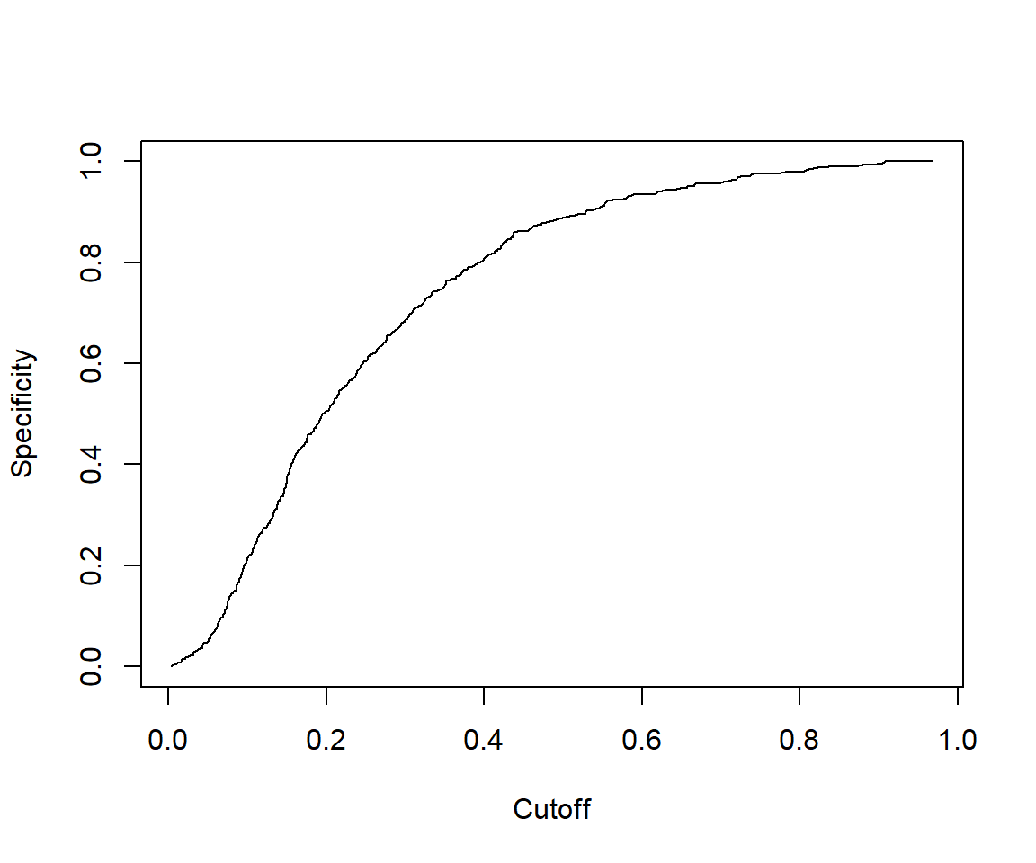
# Specificity by cutoff
perf <- performance(pred,"spec","cutoff")
plot(perf)

# Sensitivity, specificity
perf <- performance(pred, "sens", "spec")
plot(perf)

# The highest sensitivity + specificity
max(perf@x.values[[1]]+perf@y.values[[1]])

## [1] 1.467522

# The cutoff that yields the highest sensitivity + specificity
perf@alpha.values[[1]][which.max(perf@x.values[[1]]+perf@y.values[[1]])]

## [1] 0.4132145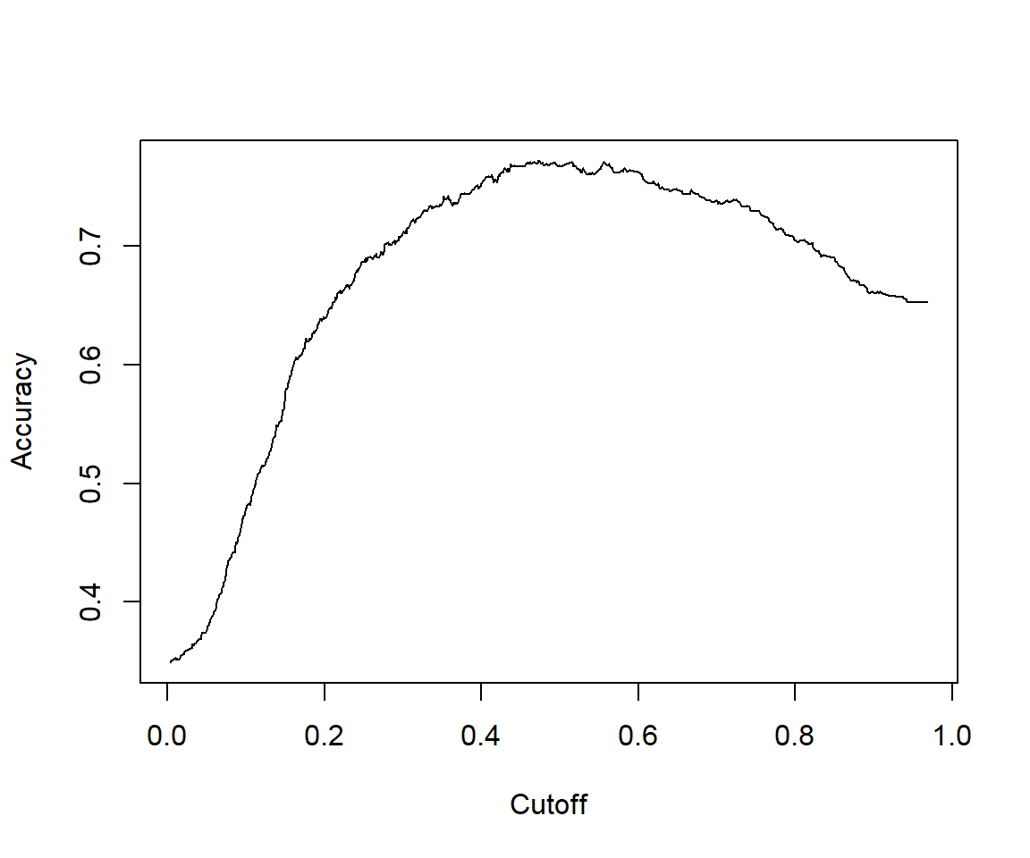

# Accuracy (all correct / all) by cutoff:
perf <- performance(pred,"acc","cutoff")
plot(perf)

# AUC
perf <- performance(pred,"auc")
perf@y.values[[1]]

## [1] 0.8114627

7.2.4.6 Calculating other model evaluation parameters

Calculate the overall Pseudo R-squared and its p-value:

• Null deviance = $2(0 - LogLikelihood(null model)) = -2LogLikelihood(null model)$
• Residual deviance = $2(0 - LogLikelihood(proposed model)) = -2LogLikelihood(proposed model)$
• chi-square value = $2(LogLikelihood(Proposed) - LogLikelihood(Null))$
• p-value = $1 - pchisq(chi-square value, df = 2-1)$

ll.null <- fitm$null.deviance/-2
ll.proposed <- fitm$deviance/-2
(ll.null - ll.proposed) / ll.null # McFadden's Pseudo R^2 = [ LL(Null) - LL(Proposed) ] / LL(Null)

## [1] 0.2258898

1 - pchisq(2*(ll.proposed - ll.null), df=(length(fitm$coefficients)-1)) # The p-value for the R^2 

## [1] 0

7.2.4.7 VIF

In multiple regression, two or more predictor variables might be correlated with each other. This situation is referred as collinearity. There is an extreme situation, called multicollinearity, where collinearity exists between three or more variables even if no pair of variables has a particularly high correlation. This means that there is redundancy between predictor variables. In the presence of multicollinearity, the solution of the regression model becomes unstable.

For a given predictor, multicollinearity can assessed by computing a score called the variance inflation factor (or VIF), which measures how much the variance of a regression coefficient is inflated due to multicollinearity in the model.

The smallest possible value of VIF is 1 (absence of multicollinearity). As a rule of thumb, a VIF value that exceeds 5 or 10 indicates a problematic amount of collinearity.

7.2.4.8 Concordance

Concordance is the percentage of predicted probability scores where the scores of actual positive’s are greater than the scores of actual negative’s. It is calculated by taking into account the scores of all possible pairs of Ones and Zeros. If the concordance of a model is 100%, it means that, by tweaking the prediction probability cutoff, we could accurately predict all of the events and non-events.

Ideally, the model-calculated-probability-scores of all actual Positive’s, (or 1) should be greater than the model-calculated-probability-scores of ALL the Negatives (or 0). Such a model is said to be perfectly concordant and a highly reliable one. This phenomenon can be measured by Concordance and Discordance.

In simpler words, of all combinations of 1-0 pairs (actuals), Concordance is the percentage of pairs, whose scores of actual positive’s are greater than the scores of actual negative’s. For a perfect model, this will be 100%. So, the higher the concordance, the better is the quality of model.

7.2.5 Model validation

7.2.5.1 Create training and test samples

The idea is that we’ll like to divide our original data into two groups: the training for training our model. While we’ll leave apart a bunch of data to check if our model is consistent. This will be our test group. And if we obtain a much worse prediction on our test set, than in our train group, then probably we’re overfitting our training data. Usually a 80–20 or 70–30% train-test split is considered reasonable.

Because there are a greater number of outcome =0 (no diabetes) than outcome =1 (diabetes), we can address this problem of class bias by building model from a balance trainingData.

library(tidyverse)
data$rn<-paste("rn",1:nrow(data),sep="") #to facilitate row selecting later
set.seed(100)  # for repeatability of samples
# Create Training data (sampling with the same fraction 0.8 for outcome =0 (no diabetes) and outcome =1 (diabetes)
trainingData<-data %>%
  group_by(outcome) %>%
  sample_frac(size=0.8) # sampling fraction the same =0.8 for outcome =0 (no diabetes) and outcome =1 (diabetes)
# Test Data is the remaining data that is not in training data 
testData <- data[!data$rn %in% trainingData$rn,]
# drop rn 
trainingData<-trainingData %>%
  select(!rn)
testData<-testData %>%
  select(!rn)
table(trainingData$outcome)

## 
##   0   1 
## 400 214

table(testData$outcome)

## 
##   0   1 
## 100  54

We can see similar proportion of outcome=0 and outcome=1 between trainingData and testData.

7.2.6 Build logitic models on training data and predict on test data

We build the same multivariable model above that uses bmi, glucose, bloodpressure to predict outcome on trainingData then validate the model on testData. The model on trainingData:

fitm.train<- glm(outcome ~ bmi + glucose + bloodpressure, data=trainingData, family="binomial")
summary(fitm.train)

## 
## Call:
## glm(formula = outcome ~ bmi + glucose + bloodpressure, family = "binomial", 
##     data = trainingData)
## 
## Coefficients:
##                Estimate Std. Error z value Pr(>|z|)    
## (Intercept)   -7.385483   0.716207 -10.312  < 2e-16 ***
## bmi            0.081722   0.015328   5.332 9.73e-08 ***
## glucose        0.036485   0.003691   9.886  < 2e-16 ***
## bloodpressure -0.006937   0.005440  -1.275    0.202    
## ---
## Signif. codes:  0 '***' 0.001 '**' 0.01 '*' 0.05 '.' 0.1 ' ' 1
## 
## (Dispersion parameter for binomial family taken to be 1)
## 
##     Null deviance: 793.94  on 613  degrees of freedom
## Residual deviance: 605.86  on 610  degrees of freedom
## AIC: 613.86
## 
## Number of Fisher Scoring iterations: 4

Make prediction and evaluate model performance on testData :

library(ROCR)
# predicted probability
predicted <- plogis(predict(fitm.train, testData))  
# or
predicted <- predict(fitm.train, testData, type="response")  

# Create a prediction object
pred <- prediction(predicted, testData$outcome)

# Create a performance object
perf <- performance(pred,"tpr","fpr")
# ROC curve
plot(perf, main="ROC")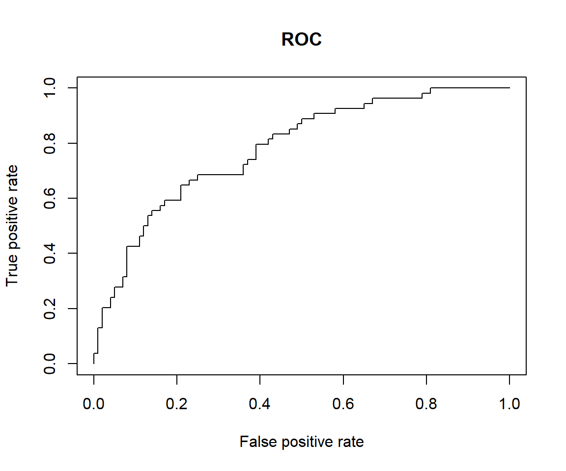

# Other performance measures
# Sensitivity by cutoff
perf <- performance(pred,"sens","cutoff")
plot(perf)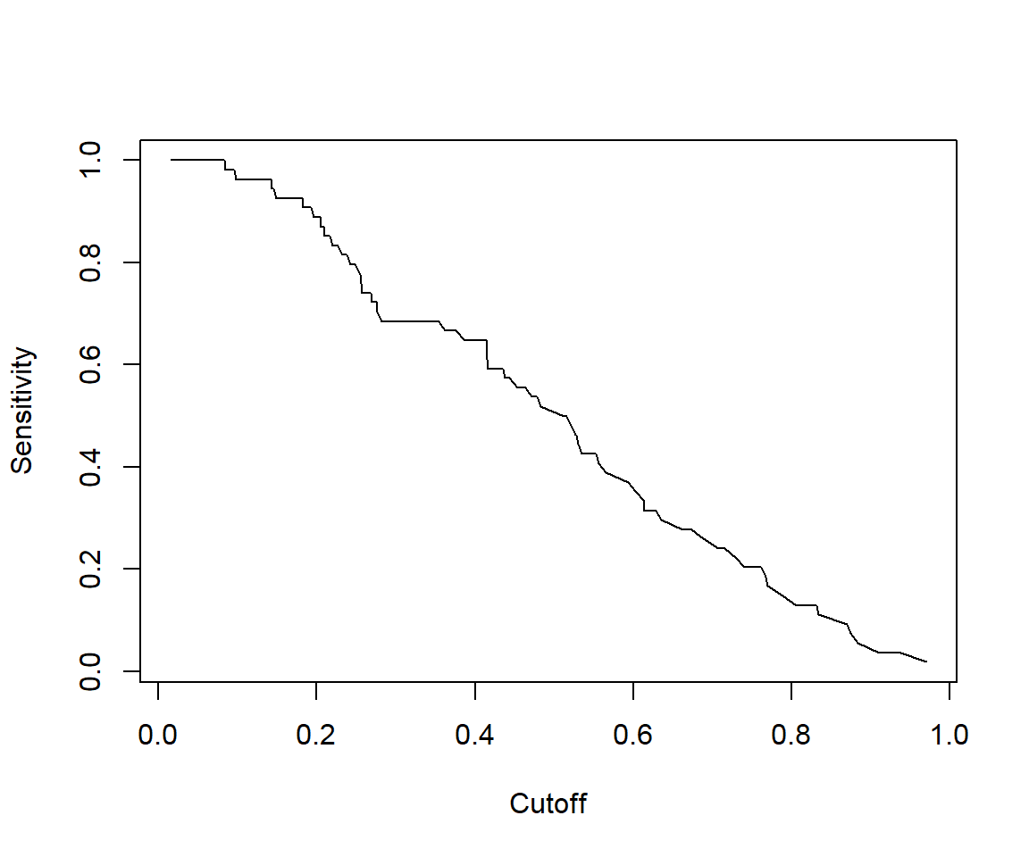

# Specificity by cutoff
perf <- performance(pred,"spec","cutoff")
plot(perf)

# Sensitivity, specificity
perf <- performance(pred, "sens", "spec")
plot(perf)

# The highest sensitivity + specificity
max(perf@x.values[[1]]+perf@y.values[[1]])

## [1] 1.438148

# The cutoff that yields the highest sensitivity + specificity
perf@alpha.values[[1]][which.max(perf@x.values[[1]]+perf@y.values[[1]])]

## [1] 0.4147078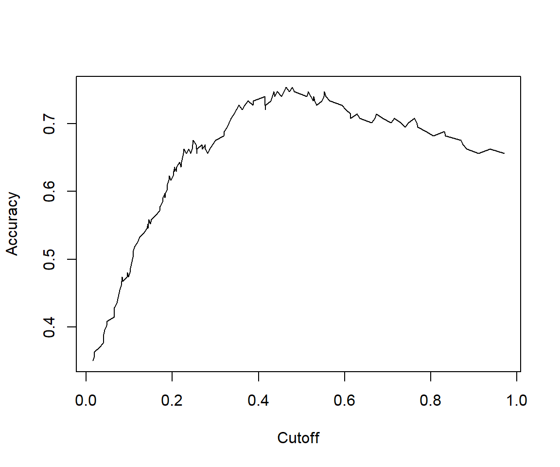

# Accuracy (all correct / all) by cutoff:
perf <- performance(pred,"acc","cutoff")
plot(perf)

# AUC
perf <- performance(pred,"auc")
perf@y.values[[1]]

## [1] 0.7809259

We can see that the model performance on testData is quite similar to model performance above.

7.3 Reference materials

The following resources have been adapted for this chapter:

• Machine Learning, by Tan C. Tran
• Logistic Regression, by Selva Prabhakaran
• Simply Explained Logistic Regression with Example in R, by Kshitiz Sirohi
• Logistic Regression in R, by Josh Starmer
• “ROCR” package vignette
• Example diabetes data

References

———. 2024b. R: A Language and Environment for Statistical Computing. Vienna, Austria: R Foundation for Statistical Computing. https://www.R-project.org/.

Sing, Tobias, Oliver Sander, Niko Beerenwinkel, and Thomas Lengauer. 2020. ROCR: Visualizing the Performance of Scoring Classifiers. http://ipa-tys.github.io/ROCR/.