Chapter 1 Summary of NCA
NCA is based on necessity causal logic. If a certain level of the condition is not present, a certain level of the outcome will not be present. Other factors cannot compensate for the missing condition. The necessary condition allows the outcome to exist, but does not produce it. This is different from sufficiency causal logic where the condition produces the outcome.
Conventional theories and methods are based on additive logic. This logic assumes that several factors contribute to the outcome and can compensate for each other. For example, conventional quantitative methods like multiple regression analysis and structural equation modeling describe the complexity of different contributing factors producing the outcome. In these models a low value of one factor can be compensated by changing another factor. When making causal interpretations with these models, factors are usually interpreted as ‘generic causes’ that can change the probability of the outcome.
Conventional quantitative methods focus on generic causes and do not cover necessity logic and are thus not able to identify necessary conditions in data sets. This was the main reason for developing NCA. NCA ensures theory-method fit when the theory includes necessity relations between factors and outcome and these relationships need to be evaluated empirically.
Conducting NCA consists of four stages:
Formulate the necessary condition hypothesis.
Collect the data.
Analyse the data.
Report the results.
Each step is explained below in more detail in sections 1.3, 1.4, 1.5, and 1.6.
In research projects and publications, NCA can be used as a stand-alone method or be used together with conventional methods such as multiple regression analysis, structural equation model, or QCA. The decision to apply NCA as a stand-alone method or a complementary method depends on the goal of the research.
1.1 NCA as stand-alone method
A researcher may have two reasons to use NCA as a stand-alone method in a particular study. First, the researcher may want to employ just a necessity view on the phenomenon of interest. He may have formulated a parsimonious ‘pure necessity theory’ (see Chapter 2) consisting of one or more necessity relations (e.g., Karwowski et al., 2016; Knol et al., 2018). To ensure theory-method fit, NCA is used for testing pure necessity theories. A regression-based method is not appropriate for this purpose. [Similarly, when a researcher wants to test a theory consisting only of generic causal relations (most current theories), a conventional probability-based method such as regression analysis should be selected and NCA is not appropriate]. A second reason for using NCA as the stand-alone method is that the researcher may want to add a necessity view to an existing generic causal theory from the literature. Without (re)testing the generic causal relationships, she may want to test whether some concepts of the theory are (also) necessary conditions.
The advantage of using NCA as a stand-alone method is that the study and its theoretical reasoning can focus on the single necessary concepts. There is no need to include other concepts (e.g., contributing factors, control variables) into the reasoning and analysis. This allows a clear story line and efficient data collection and analysis.
1.2 NCA as a complementary method
A researcher may also have reasons to use NCA in combination with other methods in a single study. The researcher may want to add a necessity view to a generic causal theory and to analyse necessity and generic relationships in combination. This can be done in two ways. First, the generic causal theory is leading and some concepts from this theory are tested for necessity. Second a combined necessity-generial causal theory is developed with both necessity and generic causal relationships between concepts.
In the first option, an existing or new generic causal theory has concepts that are considered being contributing factors that can change the probability of the outcome (including control variables). From these concepts, potential necessary conditions are selected. The necessity and generic causal relationships of these concepts with the outcome are tested with the appropriate methods and the methods are conducted successively. The integration occurs when the results are discussed. Several NCA multimethod studies that start with a generic causal theory have been reported in the literature. For example, when NCA is used in combination with (multiple) regression (e.g., Jain et al., 2022; Klimas et al., 2022; Stek & Schiele, 2021) or structural equation modeling (e.g., Della Corte et al., 2021; W. Lee & Jeong, 2021; Renner et al., 2022; Richter, Schubring, et al., 2020) “important” factors are identified with a regression-based method, and the necessity of these and other factors is analysed with NCA for identifying whether the factors are necessary or not (see section 4.5). When NCA is used in combination with Qualitative Comparative Analysis- QCA (C. S. Kopplin & Rösch, 2021; e.g., Torres & Godinho, 2022) the results of NCA are compared to the sufficient configurations that are identified by QCA (see section 4.7).
In the second option, the researcher starts the study with a combined necessity and generic causal theory. This is a complex ‘embedded necessity theory’ (see Chapter 2) that consists of both necessity and generic causal relations from the start. Some concepts may only have a generic causal but not a necessity relationship with the outcome; other concepts may be a necessary cause but not a generic cause, and yet others may be both a necessary cause and a generic cause. Embedded necessity theories that combine necessity and generic causal theorizing for describing relations are still rare. In QCA, most studies theorize from the perspective of sufficiency and test the potential necessity of the single factors, but do not include necessity theorizing from the start. Also, most studies that combine NCA with multiple regression or structural equation modeling do not theorize about necessity and generic causation in combination (for an exception see Dul, 2019). Testing embedded necessity theories requires a multimethod approach with both regression-based method and a necessity-based method.
When combining NCA with regression analysis or QCA, the order of conducting NCA and the other method is not relevant. When NCA is used in combination with structural equation modeling (SEM) the order matters. First SEM is applied followed by NCA. The reason is that the outcome of the SEM measurement model is used to define the constructs to be tested for necessity with NCA.
1.3 Formulate the necessary condition hypothesis
NCA starts with a theoretical notion that a necessity relation may exist between \(X\) (the potential condition) and \(Y\) (the outcome). This is usually done by formulating and justifying a hypothesis that is part of a theory (see Chapter 2).
NCA is mainly used in theory-testing research, which starts with formulating the theory and proceeds with empirical testing the theory with data. Hence, theory formulation comes before data collection and analysis. This is also the focus in this book. However, NCA can also be used in theory-building and exploratory research. Then formulating the theory is based on the results of the data analysis, and thus comes after it (e.g., Stek & Schiele, 2021).
1.4 Collect the data
Collecting data in NCA is not different from collecting data in general. The goal of data collection is to have scores (values, levels) for the condition \(X\) and the outcome \(Y\) for each case. The selected research design (e.g., ‘experiment’, ‘survey’, ‘case study’) must meet common quality standards. Also the selection of cases for measurement and data analysis must fit the goal of the research (e.g., random sampling, purposive sampling for specific reasons). The data must be ‘good’. This means that the data must be valid (the measurement scores reflect what they are intended to reflect) and reliable (when measurement is repeated, the results are the same).
NCA has no new requirements on collecting the data. There are a few exceptions. First, the setup of a ‘necessity experiment’ is different than the setup of a ‘sufficiency experiment’ or a common ‘average treatment effect experiment’ (see section 3.2). Second, in certain situations it is possible to sample just a single case to perform NCA (see section 3.3). Third, the way that NCA is conducted may differ depending on the types of data that are used: quantitative data (section 3.4), qualitative data (section 3.5), longitudinal data (section 3.6), and set membership scores (section 3.7). Furthermore, the identification of potential outliers is partly different from the common way of identifying outliers (see section 3.8).
1.5 Analyse the data
Data analysis is at the core of NCA. NCA’s data analysis assumes that it makes theoretically sense to analyse the data with necessity logic (see section 1.3) and that the data are meaningful (see section 1.4). For a quantitative necessary condition analysis the ‘scatter plot’ approach can be used. The scatter plot maps cases in the XY plane and NCA conducts a bivariate analysis on the scatter plot. Figure 1.1 shows an example of a scatter plot with \(X\) = Contractual detail and \(Y\) = Innovation of 48 buyer-supplier relationships for evaluating the hypothesis that Contractual detail is necessary for Innovation (Van der Valk et al., 2016).
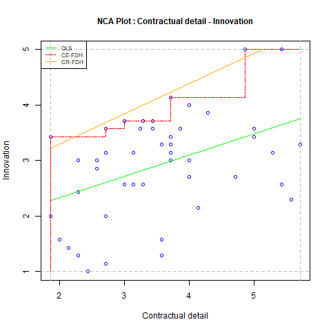
Figure 1.1: Scatter plot approach of NCA estimating the empty space in the upper left corner when \(X\) is supposed to be necessary for Y. Data from Van der Valk et al. (2016).
According to this hypothesis it is not possible to have cases with low level of Contractual detail (\(X\)) and high level of Innovation (\(Y\)). This means that the upper left corner of the scatter plot remains empty. The space without cases is called the empty space or ceiling zone. NCA draws a border line called ceiling line between the space without cases and the space with cases. Two default ceiling lines are the Ceiling Envelopment - Free Disposal Hull (CE-FDH), which is a step function that can be used when \(X\) or \(Y\) are discrete with a limited number of levels or when the border is irregular, and the Ceiling Regression - Free Disposal Hull (CR-FDH), which is a straight trend line through the upper left corner points of the CE-FDH line. When a few cases are present in the otherwise empty space the ceiling line is not entirely accurate. The ceiling-accuracy (c-accuracy) is the percentage of cases on or below the ceiling line. By definition the CE-FDH line is 100% accurate and the CR-FDH line is usually not 100% accurate. A low c-accuracy indicates that the ceiling line may not properly represent the border between empty and full space, and another ceiling line may be selected. The scope (S) is the area of the total space where cases can appear given the minimum and maximum possible values of \(X\) and \(Y\). The effect size (d) is the area of the ceiling zone (C) divided by the scope: d = C/S. The effect size can have values between 0 and 1. NCA estimates the ceiling line and its effect size from the sampled data. The statistical test of NCA consists of estimating the p value of the effect size. With the NCA software the NCA parameters can be computed.
The remaining part of this section demonstrates NCA’s data analysis by using the NCA software.
1.5.1 Prepare the analysis
For performing a (quantitative) NCA the NCA software can be used. This is a free package in R and the researcher must have access to R and RStudio. Researchers who are not familiar with R and RStudio can consult the NCA Quick Start Guide on the NCA website (https://www.erim.eur.nl). This guide explains how R and RStudio can be downloaded from internet and gives further details about the software. This demonstration uses the RStudio interface for conducting the analysis. After R and RStudio are installed and RStudio is opened, the script window is used to type and run the instructions. The first instructions for this demonstration are as follows:
#Demonstration NCA

#Install and load the NCA package
#install.packages("NCA") # to install the NCA package (only ones)
library (NCA) # load the NCA package (for each new session)
The script starts with a remark after the hashtag (#), followed by instructions to install (download) the NCA package with the install.packages function. Installing the NCA package must be done once. Afterwards, for each new NCA session, the NCA package must be loaded (activated) using the library function.
1.5.2 Load the data
Next, in this demonstration three datasets are loaded. A dataset must be organised such that rows are cases and columns are variables (condition(s) and outcome(s)). Often, data files have the .csv extension but also other data file formats can be loaded, for example .xls (Excel), .sav (SPSS) or .dta (Stata). The researcher may conduct NCA on new or existing datasets, including archived datasets that are publicly available.
#Load the data

#Data on own computer:
data1 <- read.csv("myData.csv", row.names = 1) # load and rename my dataset

#Data on internet (example Worldbank):
install.packages("WDI") #install package for loading Worldbank data
library(WDI)
data2 <- WDI (indicator = c("SH.IMM.IDPT","SP.DYN.LE00.IN"))

#Data in the NCA software:
data(nca.example2)
data3 <- nca.example2 #load the example data from the NCA package
The first dataset that is loaded is a .csv dataset. The dataset is assumed to be stored in the working directory on the user’s computer. After loading the dataset in R it is renamed as ‘data1’.
The second dataset is obtained from the internet. It is a dataset from the Worldbank website, which can be extracted with the WDI package. The first variable (indicator) that is extracted refers to the vaccination level of a country and the second to the country’s life expectancy. The vaccination level is the percentage of children aged 12-23 months who received vaccination against diphtheria, pertussis (or whooping cough), and tetanus (DPT). Life expectancy is the number of years a newborn infant would live if prevailing patterns of mortality at the time of its birth were to stay the same throughout its life.
The third dataset is part of the NCA package from version 3.1.2. and has data on 48 buyer-supplier relationships as the rows. This dataset has three conditions (Contractual detail, Goodwill trust, and Competence trust) and one outcome (Innovation). The dataset is published as Table 2 in an article entitled “When are contracts and trust are necessary for innovation in buyer-supplier relationships? A necessary condition analysis” by Van der Valk et al. (2016).
The instruction head(data3) shows the top rows of the last dataset. The first row has the variable names and the first column the names of the cases.
##   Innovation Contractual detail Goodwill trust Competence trust
## 1       3.57               3.24           2.71              4.0
## 2       3.57               2.71           2.43              3.0
## 3       1.29               2.29           4.00              4.0
## 4       2.14               4.14           3.71              4.0
## 5       1.00               2.43           3.29              3.5
## 6       3.43               1.86           3.86              4.5
1.5.3 Estimate effect size and the p value with nca_analysis
After the data are loaded the NCA analysis starts with estimating the size of the space that is expected to be empty given the hypothesis. By default, the software assumes that the expected empty space is in the upper left corner, representing the hypothesis that the presence or a high value of \(X\) is necessary for the presence of a high value of \(Y\). The software can also analyse other corners depending on whether the presence or absence of \(X\) is necessary for the presence or absence of \(Y\) (see section 1.3) by using the corner argument in nca_analysis. By default the software uses the CE-FDH and CR-FDH ceiling techniques to draw the ceiling line and to calculate the effect size. Other ceiling techniques could be selected as well using the ceilings argument in the nca_analysis function (see section 6.3.3).
The estimation of the effect size for data3 is done with the function nca_analysis. The first analysis with the name ‘model 1’ evaluates the hypothesis that Contractual detail is necessary for Innovation:
The nca_analysis instruction specifies first the dataset and then the names of the condition and the outcome. After running this instruction the analysis is done, but the output is not yet shown.
A short summary of the results can be obtained by calling model1. This prints the effect sizes of the condition for the two default ceiling lines in the console window of RStudio.
##
## ---------------------------------------------------------------------------
## ce_fdh cr_fdh
## Contractual detail 0.24 0.19
## ---------------------------------------------------------------------------The second analysis (‘model2’) shows that the condition and outcome can also be specified by their column numbers in the dataset. The results are the same.
##
## --------------------------------------------------------------------------------
## ce_fdh cr_fdh
## Contractual detail 0.24 0.19
## --------------------------------------------------------------------------------The third analysis (‘model3’) shows that multiple bivariate analyses can be done in a single run.
##
## --------------------------------------------------------------------------------
## ce_fdh cr_fdh
## Contractual detail 0.24 0.19
## Goodwill trust 0.31 0.26
## Competence trust 0.32 0.21
## --------------------------------------------------------------------------------In this example three conditions are included each representing a different necessary condition hypothesis. An analysis with multiple conditions in a single run is always done with one outcome.
The fourth analysis (‘model4’) shows that the ceiling line can be selected. In this example the CR-FDH line is selected.
#Conduct NCA with selected ceiling line
model4 <- nca_analysis(data3,2:4,1, ceilings = 'cr_fdh')
model4
##
## --------------------------------------------------------------------------------## cr_fdh
## Contractual detail 0.19
## Goodwill trust 0.26
## Competence trust 0.21
## --------------------------------------------------------------------------------The fifth analysis (‘model5’) also includes NCA’s statistical test to calculate the p value. An empty space could be a random result of variables that are actually unrelated. The p value protects the researcher from concluding that the empty space is empty because of necessity, whereas actually it is a random result of unrelated variables. The statistical test can be activated by specifying the number of permutations for the estimation of the p value in the test.rep argument of nca_analysis as follows.
## Preparing the analysis, this might take a few seconds...
## Do test for  :  ce_fdh - Contractual detailDone test for:  ce_fdh - Contractual detail
## Do test for  :  cr_fdh - Contractual detailDone test for:  cr_fdh - Contractual detail
## Do test for  :  ce_fdh - Goodwill trustDone test for:  ce_fdh - Goodwill trust
## Do test for  :  cr_fdh - Goodwill trustDone test for:  cr_fdh - Goodwill trust
## Do test for  :  ce_fdh - Competence trustDone test for:  ce_fdh - Competence trust
## Do test for : cr_fdh - Competence trustDone test for: cr_fdh - Competence trust##
## --------------------------------------------------------------------------------## ce_fdh p cr_fdh p
## Contractual detail 0.24 0.008 0.19 0.009
## Goodwill trust 0.31 0.002 0.26 0.004
## Competence trust 0.32 0.002 0.21 0.008
## --------------------------------------------------------------------------------The selection of the number of permutations is a balancing act between p value accuracy and computation time. The summary output now includes the p value for each effect size.
1.5.4 Create output with nca_output
More details of the results can be obtained with the nca_output function. The output is shown for analysis model6 that only includes Contractual detail and the CR-FDH ceiling line.
## Preparing the analysis, this might take a few seconds...
## Do test for : cr_fdh - Contractual detailDone test for: cr_fdh - Contractual detail##
## --------------------------------------------------------------------------------## --------------------------------------------------------------------------------
##
## Number of observations 48
## Scope 15.40
## Xmin 1.86
## Xmax 5.71
## Ymin 1.00
## Ymax 5.00
##
## cr_fdh
## Ceiling zone 2.893
## Effect size 0.188
## # above 2
## c-accuracy 95.8%
## Fit 79.2%
## p-value 0.009
## p-accuracy 0.002
##
## Slope 0.544
## Intercept 2.214
## Abs. ineff. 9.614
## Rel. ineff. 62.428
## Condition ineff. 15.298
## Outcome ineff. 55.642The output first displays descriptive information about the sample such as number of cases (‘observations’), the scope, and the observed extreme values of \(X\) and \(Y\). Next, the NCA parameters for the selected ceiling line are displayed including effect size, number of cases above the ceiling line, and corresponding ceiling line accuracy. The fit measure is an indication how well the ceiling line represents the border line between the space with and without cases. In this example the fit of the CR-FDH ceiling line is 79.2% (maximum fit is 100%), suggesting that the ceiling line is not very regular. Next, the p value and the accuracy of the estimated p value, which depends on the selected number of permutations in nca_analysis, are displayed. If the ceiling line is a straight line, the output also gives the slope and intercept of the ceiling line. The final four parameters are related to ‘inefficiency’, which is discussed in section 5.1.
Scatter plots can be displayed by adding the argument plots = TRUE or plotly = TRUE in the nca_output function. The regular scatter plot of ‘model 1’ can be obtained as follows:
The regular scatter plot shown in Figure 1.1 is displayed in the Plots window of RStudio.
An interactive scatter plot (‘plotly’) is displayed in the Viewer window of RStudio as follows:
The non-interactive version of this plot is shown in Figure 1.2
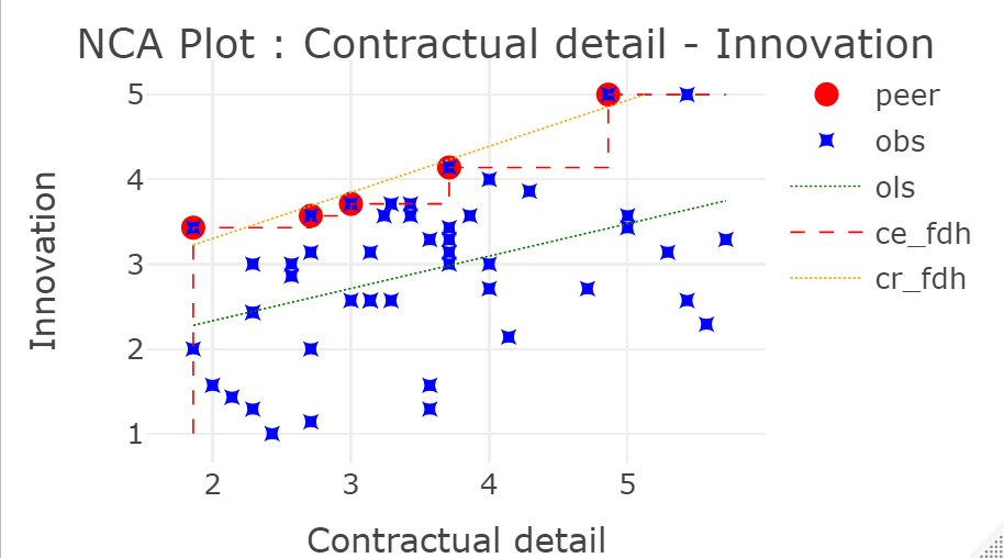
Figure 1.2: Example of a plotly scatter plot.
During inspection of the scatter plots, the researcher may observe potential outlier cases that may have a large effect on the estimated parameters. The NCA software from version 4.0.0 includes the possibility to detect and evaluate potential outliers (see section 3.8).
The scatter plots can be graphically adapted in different ways as described in section 7.3.
The results of all nca_output can be saved as a pdf file with the pdf = TRUE argument in the nca_output function.
1.5.5 Perform the bottleneck analysis with nca_output
After the effect size and its p value are computed and the scatter plots are inspected the researcher can make a judgment whether or not a necessary condition in kind (\(X\) is necessary for \(Y\)) has been identified. A common reasoning for not having identified a necessary condition is that theoretical support is lacking (no theoretically reasonable hypothesis can be formulated), or the effect size is practically irrelevant (e.g., d < 0.1), or that the empty space is likely a random result of two unrelated variables (e.g., p > 0.05). After the three conditions are satisfied (theoretical support, large effect size, small p value), the researcher may judge that there is empirical support in the present study for a necessity relationship. Then the researcher can start to conduct a necessary condition analysis in degree with the conditions that meet the three criteria. This analysis can be done with the bottleneck table. In this demonstration the three conditions and the CR-FDH ceiling line are selected for the bottleneck table analysis. The values of \(X\) and \(Y\) in the bottleneck table are ‘percentages of the range’. This means that 100 corresponds to the maximum value, 0 to the minimum value, 50% to the middle value, etc.
#Show the bottleneck table
model7 <- nca_analysis(data3, 2:4, 1, ceilings = 'cr_fdh')
nca_output(model7, bottlenecks = TRUE, summaries = FALSE)
##
## --------------------------------------------------------------------------------## --------------------------------------------------------------------------------
## Y 1 2 3
## 0 NN NN NN
## 10 NN NN NN
## 20 NN NN NN
## 30 NN NN NN
## 40 NN NN NN
## 50 NN NN NN
## 60 8.3 2.2 NN
## 70 27.4 35.2 26.0
## 80 46.5 68.2 54.0
## 90 65.6 NA 81.9
## 100 84.7 NA NATo show only the bottleneck table, the nca_output function includes the argument summaries = FALSEto suppress the text output.
The first column of the bottleneck table is a set of values of the outcome \(Y\), and the next columns show the corresponding required levels of the conditions. The table can be read row by row to find the levels of the conditions that are required for a given level of the outcome. NN means that the condition is not necessary for the corresponding level of the outcome. In the default bottleneck \(X\) and \(Y\) values are expressed as percentages of the range. As discussed in section 4.3, the values can also be expressed as actual values, percentiles and percentage of maximum, which allows useful interpretations of the bottleneck table. This section also explains why there can be NA’s in the bottleneck table. In this example there are a few NA’s, which could be replaced by the highest observed value of 5 using the argument cutoff = 1 in the nca_analysis function.
1.6 Report the results
Two types of NCA reports exist: methodological reports and application reports. In methodological reports, the method or part of the method is introduced in a specific field, often illustrated with examples from that field (Dul, Karwowski, et al., 2020; Dul, Hauff, et al., 2021; Hauff et al., 2021; Richter & Hauff, 2022; Tóth et al., 2019; Tynan et al., 2020). Introducing the NCA method in a new specific field has particularly an added value if it can be explained:
Why necessity logic is particularly useful for the field in general or for specific topics and challenges (e.g., a list of potential topics/challenges that can benefit from NCA).
That necessity thinking already (often implicitly) exists in the literature of the field (e.g., a list of necessity statements from the field).
How NCA is different from conventional methods (e.g., by explaining the steps of NCA –theory, data, data analysis, interpretation–, by referring to an example from the field).
How NCA and can give new insights to the field (e.g., an example of applying NCA to a topic from the field).
In NCA application reports the focus is on better understanding a specific phenomenon, and necessity logic and NCA are used to serve that goal. The NCA-specific parts of these application publications are (for details see Dul, 2020):
Introduction/theory: introduction of necessity logic/theory.
Methods: Description of NCA’s data analysis approach.
Results: Presentation of scatter plots and NCA parameters (e.g., effect size, p value).
Discussion: Description of the importance of including identified necessity in theory and practice (e.g., to avoid failure of the outcome or waste of efforts).
In application publications NCA can be used as a stand-alone method (section 1.1) or in combination with other methods (section 1.2).
Although NCA has already been broadly applied, there are still many fields where the NCA method has not been introduced and applied. Most likely, NCA could be applied in any of the 249 research categories defined by the Journal of Citation Reports. But currently, only about a quarter is covered, with the largest number of publications in the two categories ‘management’ and ‘business’.
1.7 Basic guidelines for good NCA practice
The guidelines are also published in Dul (2023) and Dul et al. (2023).
Based on this summary and other publications about the NCA methodology (Dul, 2016b, 2020, 2023; Dul, Van der Laan, et al., 2020), basic guidelines for good NCA practice can be formulated (Table 1.1). These general guidelines can support researchers and reviewers of research in conducting, reporting and evaluating NCA studies, and can help to ensure good quality of NCA applications.
| Topic | Chapter |
|---|---|
| Theoretical justification | |
| Explain why X can be necessary for Y. | Ch. 2 |
| Formulate the relationship between X and Y in terms of a necessity hypothesis (e.g., in terms of “X is necessary for Y”). | |
| In explorative research, theoretically justify a necessary condition that is found ex post. | |
| Meaningful data | |
| Use a good sample. | Ch. 3 |
| Use valid and reliable scores of X and Y (e.g., by using common approaches for evaluation of validity and reliability). | |
| Scatter plot | |
| Show the scatter plot (or contingency table) of all conditions that are evaluated for necessity. | Ch. 4 |
| Visually inspect the scatter plot (e.g., pattern of the border, potential outliers). | |
| Ceiling line | |
| Select the ceiling(s) based on the number of levels of X and Y and the expected or visually observed (non-)linearity of the border. | Ch. 4 |
| Only show the selected ceiling lines in the scatter plot. Do not show the two (default) ceiling lines if these are not selected for the analysis. | |
| Effect size | |
| Report the estimated effect size. | Ch. 4 |
| Evaluate the practical relevance of the effect size (e.g., threshold level > 0.1). | |
| Statistical test | |
| Report the estimated p-value. | Ch. 6 |
| Evaluate the statistical relevance of the effect size (e.g., threshold level < 0.05). | |
| Bottleneck analysis (necessity in degree) | |
| Present the bottleneck table for the non-rejected necessary conditions. | Ch. 4 |
| Decide how to present the bottleneck table (e.g., using percentage of range, actual values, or percentiles). | |
| Descriptions of NCA | |
| Refer to NCA as a method (including logic/theory, data analysis and statistical testing), not just as a statistical tool or data analysis technique. | |
| Acknowledge that: | |
| • NCA’s necessity analysis differs from fsQCA’s necessity analysis. | |
| • NCA differs from a “moderation analysis” in regression analysis. | |
| • NCA is not a robustness test for other methods. | |
| Properly describe elements of NCA, e.g.: | |
| • Use only necessity wordings to describe the necessity relationship between X and Y (avoid imprecise or general words like (cor)related, associated, and incorrect sufficiency-based words like produce, explain). | |
| • Refer to NCA’s statistical test as a permutation test (avoid incorrect descriptions like bootstrapping, (Monte Carlo) simulation, robustness check, or t-test). | |
| • Use the name ‘multiple NCA’ or ‘multiple bivariate NCA’ rather than ‘multivariate NCA’ when several conditions are analysed in one run. | |
1.8 SCoRe-NCA. A checklist for reviewing an NCA publication
An NCA publication can be categorized as:
Empirical publication: Application of NCA’s necessity logic and data analysis approach with empirical (or simulated) data. The goal is to provide a theoretical, empirical, methodological, practical contribution (or a combination) by using data.
Theoretical publication: Use of NCA’s necessity logic for theory development without using data and NCA’s data analysis. Specific characteristics of NCA’s necessity logic are used in the publication, for example NCA’s ‘conditional logic with a causal assumption’, NCA’s ‘necessity in degree’, or NCA’s ‘typicality’ necessity perspective.
Methodological publication: The Description, explanation, illustration or further development of the NCA method.
Referencing publication: reference to (elements of) NCA, such as referencing (but not using) NCA’s necessity logic or to (elements of) NCA’s data analysis approach, or suggesting the use of NCA for future research (for example, in a review article or discussion section of a non-NCA publication).
This section provides a draft checklist to evaluate the quality of an empirical NCA publication (the final checklist will be published in Dul (2026); please send your comments on the draft checklist to jdul@rsm.nl). The checklist can be used by authors to prepare their research, ensuring the proper application of NCA, and the proper reporting of NCA results. It can also be used by peers, reviewers, and editors to evaluate the quality of the publication and provide constructive feedback.
The checklist builds on the published basic guidelines for conducting and reporting NCA (Dul et al., 2023), and recent developments in NCA such as about NCA’s causality (Dul, 2024a), necessity theorizing (Bokrantz & Dul, 2023), NCA’s robustness checks (Section 4.4), sampling for NCA (Dul, 2024b), use of archival data in NCA (Dul et al., 2024), and developments related on the application of NCA in combination with QCA (Dul (2022); Section 4.7) or PLS-SEM (Hauff et al., 2024; Richter, Hauff, Ringle, et al., 2023). Therefore, the checklist provides an up-to-date set of recommendations for a high-level application of NCA, based on the current knowledge about NCA.
Following the structure of a ‘standard’ academic publication, the checklist has six sections (Introduction/General, Theory/Hypotheses, Methods-data, Methods-data analysis, Results, Discussion) each with about 5-10 NCA items that need to be addressed in an empirical NCA publication. The items have different priority levels. Some items are essential (‘must-haves’) that must be addressed in any NCA publication. Other items are important (‘should haves’) to increase the quality of the publication, and yet other items are the ‘nice-to-haves’. When addressing all items, the publication meets the highest quality standard, for example for being published in a high-ranked journal. Some items can be easily addressed, others need more reflection. For each item, requirements, recommendations, and sources for further reading are provided.
The SCoRe-NCA checklist is a tool for authors, editors and reviewers to evaluate the quality of an NCA study. The acronym refers to S: Strengthening (Theoretical Rigor), Co: Conducting (Data & Analysis Quality), and Re: Reporting (Transparency) which topics are covered in the checklist.
The SCoRe-NCA can be used for any empirical publication that uses NCA, whether it is the only method that is applied, or that NCA is used in combination with other methods. In Section 4.6 some specific recommendations are given for applying NCA in combination with SEM (and in particular PLS-SEM) as the number of PLS-SEM studies that also apply NCA is rapidly growing.
In the checklist below, the user can select all items or a selection of items for specific publication sections or specific priority levels.
The following table allows this interaction with the checklist:
| Section | Priority | Item | Question | Recommendation | Further reading |
|---|---|---|---|---|---|
| Introduction/General | Must-have | 1 | Are the goals and contributions of applying NCA explicitly stated? | State the primary and (possibly) secondary goals and contributions of the NCA application, such as theoretical contribution: (formulating necessity hypotheses before data analysis and testing them or in exploration formulating necessity hypotheses after data analysis); empirical contribution (analyzing data from a necessity perspective without additional theorizing, e.g., description, prediction, exploration, replication, reproduction, or generalization); methodological contribution (applying NCA or a certain aspect of it for the first time in a particular field); practical contribution (using results of NCA, e.g., for an accepted hypothesis: practitioners must act on bottlenecks to be effective and avoid waste; no compensation possible, or for a rejected hypothesis: compensation is possible when the condition is absent). | Articles: Bokrantz & Dul (2023); Dul (2024a); Hollenbeck & Wright (2017); Shmueli (2010); Köhler & Cortina (2023); Bergh et al. (2022); This book: Sections 2.4 and 2.2.4 |
| Introduction/General | Must-have | 2 | When referring to necessity, are only words that correctly describe a necessity relationship used? | Refer to necessity only by using words that describe a necessity relationship. Avoid imprecise descriptions like X (cor)relates with Y, X is associated with Y, X affects Y, X causes Y, etc. Avoidincorrect sufficiency-based descriptions like X produces Y, X drives Y, X increase/decreases Y, etc. | This book: Table 2.1 |
| Introduction/General | Must-have | 3 | Is it explained that NCA is a method that consists of both a specific causal logic and the related data analysis technique? | Refer to NCA as a method that combines necessity causality (rather than common probabilistic or configurational causality) and a related data analysis technique (ensuring theory-method fit). NCA is not just a data analysis technique or statistical tool. | Article: Dul (2024a) |
| Introduction/General | Must-have | 4 | Is a proper comparison made between NCA’s causal perspective and conventional causal perspective (e.g., when regression analysis or QCA is used)? | When comparing necessity (causal) logic and NCA with causal interpretations of conventional regression-based/statistical approaches, use the term “probabilistic sufficiency” and not just “sufficiency” for the latter approaches, as “sufficiency” suggests (quasi-)determinism, like in QCA configurational sufficiency logic. This recommendation is often violated in studies that combine NCA with PLS-SEM. When NCA is compared with QCA’s necessity analysis, use the term “necessity analysis of QCA” for the latter (and not “NCA”) and explain the differences between the necessity analysis of QCA (only in kind) and that of NCA (also in degree). | Articles: Dul (2024a); Dul (2016a); Vis & Dul (2018); Dul (2022); This book: Sections 4.6 and 4.7 |
| Introduction/General | Must-have | 5 | Is NCA explained as a method with a different perspective on causality and data analysis, and not as a robustness or confirmation test for other methods (e.g., regression analysis or QCA), and vice versa? | Use NCA as an approach with a different perspective on causality and therefore a different way of data analysis. NCA is not a robustness or a confirmation test for other methods (and vice versa). | Article: Dul (2024a) |
| Introduction/General | Nice-to-have | 6 | If the necessity analysis is a prominent part of the publication, does the title (and abstract) reflect this necessity perspective/NCA? | If an important part of the publication and/or its conclusions are based on necessity logic and NCA, include in the title (and abstract) words that reflect necessity logic or NCA. | This book: Table 2.1 |
| Theory/Hypotheses | Must-have | 7 | Is the hypothesized necessity relationship explicitly formulated as: “X is necessary for Y”, or similar? | Formulate the necessity relationship explicitly as a necessary condition hypothesis: “X is necessary for Y”. For hypothesis testing research this is done before data analysis; for hypothesis building/exploration research this is done after data analysis when a potential necessity relationship is found. | This book: Sections 2.2 and 4.6 |
| Theory/Hypotheses | Must-have | 8 | Is the theoretical domain of the necessity hypothesis specified? | Specify the theoretical domain of the necessity theory/hypothesis where it is claimed/expected that necessity will hold, given its boundary conditions. Note that the theoretical domain is usually larger than a population from which a sample is drawn, or cases are selected. The theoretical domain may be better specified after doing a thought experiment. | This book: Sections 2.1 and 2.2.2 |
| Theory/Hypotheses | Must-have | 9 | Is it convincingly explained WHY X is necessary for Y using necessity causal logic to justify the necessity hypothesis? | Explain why X is necessary for Y using necessity logic (why cases with the outcome will almost always have the condition (if Y then X); why cases without the condition rarely have the outcome (if no X then no Y); why the absence of the condition cannot be compensated or substituted by another factor. Consider doing and reporting the results of a thought experiment (searching for exceptions) in the development of a necessity hypothesis. Note that formulating and justifying a necessity relationship is a creative process, supported by literature and experiences of academics and practitioners. | This book: Sections 2.2.2 and 4.6 |
| Theory/Hypotheses | Should-have | 10 | Is the existing literature about the relationship between X and Y re-considered from a necessity causal perspective? | Review existing literature (that commonly describes probabilistic relationships between your variables X and Y), to find hints for necessity causality. Avoid just describing, summarizing, or referring to probabilistic findings/ideas. Where possible, include quotes in the literature that hint to necessity logic. Avoid using sufficiency/probabilistic causal logic for making a justification for necessity causal logic. | This book: Table 2.1 |
| Theory/Hypotheses | Should-have | 11 | Is the “direction” of the necessity relationship specified? | If the “direction” of the necessity relationship differs from presence/high level of X is necessary for presence/high level of Y, formulate the “direction” of necessity in the necessary condition hypothesis by adding presence/high level or absence/low level of X and Y. | This book: Section 2.2.3 |
| Theory/Hypotheses | Nice-to-have | 12 | Is an “nc” symbol added above the arrow in a figure that represents a necessity relationship? | In a figure representing an (expected) necessity relationship between two variables using an arrow, add a relevant symbol (+nc+, or -nc+ or -nc- or +nc-) near the arrow to show the direction of necessity. | This book: Section 2.2.3 |
| Theory/Hypotheses | Nice-to-have | 13 | Is the focal unit of the necessity hypothesis specified? | If this is not obvious from the definition of the theoretical domain, specify the focal unit of the necessity theory/hypothesis (is the necessity theory/hypothesis about a person, team, organization, project, dyad, country, etc.). | This book: Section 2.1 |
| Theory/Hypotheses | Nice-to-have | 14 | Is the temporal order of X and Y specified? | If this is no obvious, include a plausible explanation of the temporal order (first X then Y) in the description of why the necessity causal relationship exists. If the data support “X is necessary for Y” it should be explained why the alternative explanation, “Y is sufficient for X” is not plausible. | This book: Section 2.3.1 |
| Theory/Hypotheses | Nice-to-have | 15 | Is it specified if rare exceptions are allowed? | When formulating necessity theory/hypotheses explain if rare exceptions are allowed (typicality perspective of necessity: “almost always necessary’”) or not (deterministic perspective on necessity). | Article: Dul (2024a) |
| Methods - data | Must-have | 16 | Are proper common methods used for collecting data; 1. research design (experiment, large N observational study, small N observational study); 2. sampling or case selection from the theoretical domain; 3. measurement for getting scores of X and Y in the hypothesis; 4. practically interpretable? | Specify: 1. the research design which can be the experiment (where X is manipulated and Y is observed), the large N observational study (where X and Y are observed), or the small N cases study (where X and Y are observed); 2. the sampling approach (e.g. probability sampling) or case selection approach (e.g., purposeful selection) from the theoretical domain; 3. the measurement approach to ensure valid, reliable and meaningful data; 4. the practical meaning of the levels of X and Y. Data are input to NCA, not part of NCA. | This book: Sections 3.2, 3.3, 3.4, 3.5, 3.6, and 3.7 |
| Methods - data | Must-have | 17 | For simulation studies: are bounded X and Y variables used for obtaining artificial data? | For data generated by simulation, ensure that the variables X and Y are bounded (have minimum and maximum values). For example, sampling from uniform or truncated normal distributed data are eligible, but not sampling from normal distributed data. | This book: Section 6.3.1 |
| Methods - data | Must-have | 18 | Are only data transformations that align with NCA employed? | Explain possible data transformations. NCA only allows linear data transformation (e.g., min-max transformation, normalization, standardization, or percentage transformation), unless non-linear transformed data validly represent X and Y of the hypothesis. NCA’s data analysis does not require data transformation. Often non-transformed data are more meaningful and better interpretable (e.g., levels of a Likert scale) than transformed data. This particularly applies to NCA’s necessity in degree for interpreting that a certain level of X is necessary for a certain level of Y. Do not conduct non-linear data transformation (e.g., log-transformation, logistic transformation) unless only the transformed X or Y represent the concepts X and Y in the necessity hypothesis. This recommendation is often violated in studies that combine NCA with QCA when the logistic transformation (‘S curve’) is applied mechanistically for calibration purposes. | This book: Sections 3.1 and 4.6 |
| Methods - data | Should-have | 19 | For small N qualitative research: is proper purposive case selection applied? | For small N qualitative NCA research: Specify the purposive selection of cases from the theoretical domain: based on presence of Y or on absence of X. If a different type of purposive case selection, random case selection, or convenience case selection is used, specify the type of case selection and its limitations. | Article: Dul (2024b); This book: Section 3.3.1 |
| Methods - data | Nice-to-have | 20 | For large N quantitative research: are the results of a pre-study power analysis reported? | In large N quantitative research: Report if a pre-study power analysis was done to estimate the required sample size for finding necessity if it exists. Note that doing a post-hoc power analysis makes no sense for the present study but could inform future studies only. | Article: Dul (2024b); This book: Section 6.3.2 |
| Methods - data analysis | Must-have | 21 | Is the selected primary ceiling line specified and justified? | Specify and justify the primary selection of the ceiling line (e.g., CE-FDH when X or Y is discrete or when the ceiling line is expected to be non-linear; CR-FDH when X and Y are continuous or when the ceiling line is expected to be straight). | This book: Sections 4.1.2, 4.4.1, and 4.6 |
| Methods - data analysis | Must-have | 22 | Is the threshold value for the effect size specified and justified? | Specify and justify the selection of the threshold value for necessity effect size for identifying necessity in kind. This threshold depends on the specific context of the study. If no argument is available for a specific value, a common benchmark value may be used (d = 0.10). | Article: Dul (2016b); This book: Sections 4.2, 4.4.2 |
| Methods - data analysis | Should-have | 23 | Is NCA’s statistical test correctly described, and the threshold p value specified? | Refer to NCA’s statistical test as a permutation test (avoid incorrect descriptions like bootstrapping, (Monte Carlo) simulation, robustness check, or t-test). Specify the number of permutations that were selected from the permutation distribution (commonly 10,000), and the threshold p value that is selected (commonly 0.05). | Article: Dul, Van der Laan, et al. (2020); This book: Section 6.2 |
| Methods - data analysis | Should-have | 24 | Are NCA parameters including ceiling zone, feasible area, scope, and effect size properly described? | Make sure that the feasible area is described as the area under the ceiling where points/cases are possible. Avoid names such as “full area”. Describe the scope correctly as the area bounded by the minimum and maximum values of X and Y (the bounding rectangle). Specify and justify the selection of the scope. By default, the empirical scope can be used, but reasons may exist to select a theoretical scope (e.g. representing the minimum and maximum values of the scales that are used for scoring X and Y; comparing effect sizes as in simulations). | This book: Section 5.1 |
| Methods - data analysis | Nice-to-have | 25 | Is a proper name used for analyzing several necessary conditions simultaneously? | When several conditions are analyzed, use the name “multiple NCA” rather than “multivariate NCA”. | This book: Section 5.2 |
| Methods - data analysis | Nice-to-have | 26 | Is the software, including its version number, that is used for conducting NCA specified? | Specify which software and which version of the software was used to conduct NCA. | This book: Section 7.1 |
| Methods - data analysis | Nice-to-have | 27 | Is a short description of NCA’s data analysis approach provided? | Provide to readers who are unfamiliar with NCA’s data analysis approach a short description of the NCA’s main elements (ceiling line, ceiling zone, scope, effect size) and refer to references for further reading. | This book: Chapter 1; Appendix in Dul (2024a) |
| Results | Must-have | 28 | Are XY tables or XY plots of all tested/explored relationships shown? | Show in the main text or an appendix the XY tables or XY plots of all tested/explored relationships such that the reader can inspect the patterns. | This book: Sections 4.1 and 4.6 |
| Results | Must-have | 29 | For large N quantitative research: are the effect size and its p value properly reported? | Report the estimated effect size preferably with two decimal places (e.g., d = 0.09 or d = 0.11), ensuring that the two digits have meaningful information about the precision of the effect size (e.g., for making a comparison with a threshold, e.g., d = 0.10 possible), and to avoid suggesting an unwarranted level of accuracy. Report the estimated p value preferably with three decimal places (e.g., p = 0.049 or p = 0.051), ensuring that the three digits have meaningful information about the precision of the p value. | NA |
| Results | Must-have | 30 | Is the conclusion about necessity in kind based on three criteria: theoretical justification, effect size, and p value? | Conclude about necessity in kind using three criteria: 1. theoretical justification (the hypothesis); 2. Effect size large enough (above the selected threshold value), p value small enough (below the selected threshold value). | This book: Sections 1.5.5 and 4.6 |
| Results | Must-have | 31 | For multiple necessary conditions: Is the bottleneck table reported? | Report the bottleneck table when multiple necessary conditions are not rejected to evaluate for which level of Y, which levels of the X’s are required. | This book: Section 4.3 |
| Results | Should-have | 32 | Is only the primary ceiling line shown in the XY plot? | Show only the primary ceiling line in the XY plot that is used for the main analysis for drawing a conclusion about the necessity relationship. | NA |
| Results | Should-have | 33 | Are the type of values used in the bottleneck analysis justified? | Justify the type of values for X and Y (percentage of range, actual values, percentiles). In particular, the actual values of Y and percentile values of X might be informative about the percentage of cases not able to achieve a target outcome. | This book: Section 4.3 |
| Results | Should-have | 34 | Are the results of the robustness checks summarized? | Summarize the results of the robustness checks: is the conclusion about necessity sensitive for choices by the researcher regarding ceiling line, effect size threshold, p value threshold, scope (theoretical, empirical), and removing/keeping outliers (ceiling and scope outliers). Conclude if the results are robust or fragile. | This book: Section 4.4 |
| Results | Nice-to-have | 35 | Are the results of a visual inspection of XY plots reported? | Report that a visual inspection of XY plots was done for all hypothesized/explored necessity relations regarding (1) the expected empty corner given the hypothesis, (2) what is the preferred primary ceiling line (e.g., irregular or straight border), and (3) if potential outliers exist (ceiling and scope outliers). | This book: Section 4.1 |
| Results | Nice-to-have | 36 | If applicable: is the meaning of ‘NN’ and ‘NA’ in the bottleneck table explained? | Explain the meaning of ‘NN’ and ‘NA’ in the bottleneck table. | This book: Section 4.3 |
| Discussion | Must-have | 37 | Is it explained why all tested necessary conditions were accepted or rejected? | Summarize the results of using NCA in terms of which necessary conditions were tested/explored, and which were (not) rejected. Explain what could be a theoretical reason of it (refer to the reasoning for the hypothesis formulation). | This book: Section 4.7 |
| Discussion | Must-have | 38 | For multimethod research: is it explained how the results of NCA and of other methods complement each other? | When NCA is used in combination with another methods (e.g., regression-based methods or QCA), report how the results of NCA and of the other method complement each other. | This book: Sections 4.5 and 4.6 |
| Discussion | Must-have | 39 | Referring to the contribution (see introduction): is it discussed if the added value has been realized and what key insights were gained? | For a theoretical, empirical, methodological and/or practical contribution (see introduction), discuss if the added value has been realized and what key insights were gained. | NA |
| Discussion | Should-have | 40 | Is an interpretation given of the results of the bottleneck analysis in terms of necessity in degree? | Give an interpretation of necessity in degree using the results of the bottleneck analysis. For example, explain what level of X is necessary for what target level of Y. | This book: Section 4.3 |
| Discussion | Should-have | 41 | Are limitations of applying NCA mentioned? | Mention general limitations of NCA (e.g., only focus on necessity; potential sensitivity to outliers), and specific limitations of applying NCA in the current study. | NA |
| Discussion | Should-have | 42 | Are potential future research directions with NCA discussed? | Discuss potential future research directions with NCA, for example conducting studies in other parts of the theoretical domain to verify generalizability of the current findings, or applying NCA in related substantive areas that could benefit from the necessity causal perspective. | Article: Köhler & Cortina (2023) |