Chapter 5 NCA’s mathematical backgrounds
5.1 Formal mathematical expression
Necessary Condition Analysis describes the boundary between the area in the \(XY\)-plane where cases \((X,Y)\) are possible (‘feasible area’) and the area where cases are not possible (‘empty space’). NCA calls this boundary the ceiling. The cases are on or below the ceiling, but not above it. The ceiling is a sharp border indicating that for a certain level of \(X\) it is possible to have values less than or equal to the ceiling value of \(Y\), but it is not possible to have values above the ceiling value of \(Y\). This means that \(X\) is necessary for \(Y\). However, \(X\) is usually not sufficient for \(Y\) because normally there are cases below the ceiling. The ceiling represents the constraining effect of \(X\) on \(Y\): without a certain level of \(X\) it is not possible to have a certain level of Y. The basic mathematical expression of NCA is therefore \[\begin{equation} \tag{5.1} Y \leq f(X) \end{equation}\] where \(f(X)\) is the ceiling function.
Figure 5.1 shows an example of a non-decreasing piecewise linear ceiling function where \(X\) and \(Y\) are bounded (have a minimum and a maximum value). The function indicates that possible outcomes of \(Y\) corresponding to a given \(X\)-value is an interval \([y_{min},f(X)]\).
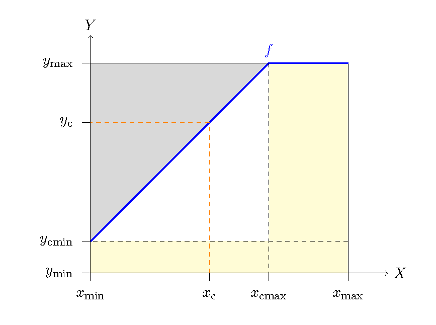
Figure 5.1: A linear ceiling function (blue).
When the ceiling is non-decreasing, the necessary condition of \(X\) for \(Y\) for a value equal to a specific value \(y_{c}\), can now be expressed as \[\begin{equation} \tag{5.2} Y = y_{c} \quad \Rightarrow \quad X \geq f^{-1} (y_{c}) \end{equation}\] where \(f^{-1}\) is the inverse of \(f\) and \(C\) is a point on the ceiling line. So, rephrasing, it is needed that \(x \geq f^{-1}(y_{c})\) in order to observe a value for \(Y\) equal to \(y_{c}\).
The assumption of bounded \(X\) and \(Y\) allows the definition and calculation of the NCA effect size (see section 5.1.1) and other NCA parameters (e.g., 5.1.2). The assumption of a non-decreasing ceiling allows the use of the bottleneck table as explained in section 4.3. Linearity is not a requirement for NCA.
5.1.1 Effect size
When \(X\) and \(Y\) are bounded, it is possible to define the effect size of a necessary condition. In Figure 5.1 the lines \(X=x_{{min}}\), \(X=x_{{max}}\), \(Y=y_{min}\) and \(Y=y_{{max}}\) define the space of possible values for \(X\) and \(Y\). The area between these lines is called the scope. The difference between the absolute maximum possible \(Y\)-value (\(Y=y_{\text{max}}\)) and the maximum possible \(Y\)-value for a given \(X\) (\(Y=y_{c}\)) can be considered as the constraint that \(X\) puts on \(Y\). The slope of the line expresses the change in constraint under varying \(X=x\). The maximum constraint for absence of values of \(Y\) occurs for \(X = x_{min}\). The effect builds up with increasing \(X\) at a rate determined by the slope of the ceiling line. The total effect is then the surface area between the ceiling line and the maximum possible \(Y\). This area is called the ceiling zone. The effect size of a necessary condition is the ceiling zone divided by the scope, which takes values between 0 and 1. When the minimum and maximum \(X\) and \(Y\) values are theoretically presumed values, the scope is called the theoretical scope. When the minimum and maximum \(X\) and \(Y\) values are empirically observed, the scope is called the empirical scope.
5.1.2 Necessity inefficiency
When \((x_{c},y_{c})\) is a point on the ceiling line and \(x\leq x_{c}\), then \(x\) is a bottleneck for \(y \geq y_{c}\). Only an increased value of \(x\) towards \(x = x_{c}\) enables a value \(y = y_{c}\). For reaching the value of \(y = y_{max}\) it is necessary to have a value of \(x\geq x_{cmax}\), where \(x_{cmax}\) is the value of \(x\) of the point where the ceiling line crosses the \(y = y_{max}\) line. For enabling the maximum possible \(y\) value, \(x\) should be \(x = x_{cmax}\). There is no need to increase \(x\) beyond \(x = x_{cmax}\) for enabling \(y = y_{max}\) , as \(y\) is not constrained anymore. This is called ‘inefficiency’ regarding enabling the maximum outcome.
Condition inefficiency specifies the extent to which \(x\) does not constrain \(y\) for levels of \(x_{cmax}\leq x\leq x_{max}\). Only for \(x_{min}\leq x\leq x_{cmax}\), \(x\) constrains \(y\) (ceiling line exists for \(x_{min} \leq x\leq x_{cmax}\)). Condition efficiency is expressed as a percentage: \((x_{max}-x_{cmax})/(x_{max}-x_{min})*100\%\). Condition inefficiency is 0% if \(x\) constrains \(y\) for all values of \(x\); condition inefficiency is 100% if \(x\) does not constrain \(y\) for any value of \(x\).
Similarly, outcome inefficiency specifies the extent to which \(y\) is not constrained by \(x\) for lower levels of \(y_{min}\leq y\leq y_{cmin}\), where \(y_{cmin}\) is the value of \(y\) of the point where the ceiling line crosses the \(x = x_{min}\) line. Only for \(y_{cmin}\leq y\leq y_{max}\), \(y\) is constrained by \(x\) (ceiling line exists for \(y_{cmin}\leq y\leq y_{max}\)). Outcome efficiency is expressed as a percentage: \((y_{cmin}-y_{min})/(y_{max}-y_{min})*100\%\). Outcome inefficiency is 0% if \(x\) constrains \(y\) for all values of \(y\); outcome inefficiency is 100% if \(y\) is not constrained for any value of \(x\).
5.2 Multiple NCA
NCA considers one condition at a time. With several conditions, NCA conducts successive analyses by considering the ceilings in the separate \(X_iY\)planes. For example, with two conditions (\(X_1\) and \(X_2\)), two separate analyses are done: one in the \(X_1Y\) plane (\(X_1Y\) scatter plot) and the other one in the \(X_2Y\) plane (\(X_2Y\) scatter plot). In other words, in the three dimensional space \((X_1,X_2,Y\)) NCA puts a blanket on the data (ceiling surface) and takes the orthogonal projection of the ceiling surface on the \(X_1Y\) plane and the projection of the ceiling surface on the \(X_2Y\) plane. Therefore, each condition has an independent ceiling line. The two ceiling lines are \(f_1(X_1)\) for \(X_1\) and \(f_2(X_2)\) for \(X_2\). Consequently, for a given value \(Y = y_c\) two conditions must be satisfied: \(X_1 \geq x_{1c}\) AND \(X_2 \geq x_{2c}\). Therefore, the maximum possible \(Y = y_c\) for given values \(X_1 = x_{1c}\), and \(X_2= x_{2c}\) is
\[\begin{equation} \tag{5.3} y_c = min \{f_1(x_{1c}), f_2(x_{2c})\} \end{equation}\]
where \(y_c\) is a particular outcome value, \(x_{ic}\) is the necessary \(X\)-value of the i-th condition, \(f_i\) is the ceiling line of the i-th condition and \(C\) is a point on the ceiling line. With more than two conditions there is a multidimensional ceiling with projections \(f_i(X_i)\). The mathematical descriptions of a necessary AND combination of multiple necessary conditions is: \(X_i \geq x_{ic}\) for \(Y = y_c\) and the maximum possible \(Y = y_c\) for given values of \(X_i = x_{ic}\) is
\[\begin{equation} \tag{5.4} y_c = min \{f_i(X_i)\} \end{equation}\]
where \(y_c\) is a particular outcome value, \(x_{ic}\) is the necessary \(X\)-value of the i-th condition, \(f_i\) is the ceiling line of the i-th condition and \(C\) is a point on the ceiling line.
Although NCA performs separate analyses for each condition, in NCA’s bottleneck table (see section 4.3), the separate analyses are combined and considered in combination. This allows answering the question: “What levels \(x_{ic}\) of \(X_i\) are necessary for a particular level \(Y = y_c\)”? or “For given levels \(x_{ic}\) of \(X_i\) what is the maximum possible level \(y_c\) of \(Y\)”.
There are several reasons why NCA analyses projections of the multidimensional ceiling.
The first reason is the fundamental choice to focus on single factors that are necessary for an outcome. This makes NCA different from conventional analyses. Conventional approaches study multi-causal phenomena by considering a combination of factors and their interplay as a whole. A multivariate analysis is the realistic option for predicting the presence of an outcome, because normally only a combination of factors and not a single factor can produce the outcome. However, for predicting the absence of an outcome is it realistic to study a single factor (the necessary condition or ‘bottleneck’) that can prevent the outcome to exist when the level is too low. Therefore, it is possible and useful to study the necessity of single factors for an outcome with projections.
The second reason is that NCA makes statements about single factors that are necessary independently of other factors. Thus, the necessity of a single factor does not depend on the level of other factors. This allows for a “pure” and straightforward interpretation of necessity: “the factor is necessary” rather than “the factor is necessary depending on other factors”. Such pure necessity statement holds independently of other factors. However, the context where the necessity statement holds is usually not unlimited. The domain where the generic necessary condition is supposed to hold must be defined as the ‘theoretical domain’ of the necessity theory. Such specification of the theoretical domain (sometime called “scope conditions”) must be part of any theory and related hypotheses (for further discussion and examples, see Dul (2020)).
A third reason is that NCA wants to contribute to parsimonious (simple) theories: avoiding that theories become complex, not understandable and (thus) less useful. This is a general goal of theory building in applied sciences. NCA is an elegant way of reducing complexity, in particular in situations where it is hard or impossible to predict the outcome (e.g., when the explained variance of regression models is low) or when a good prediction is only possible with a very complex model.
The fourth reason is that practical recommendations from identified single necessary conditions are immediately clear and useful: “for a given outcome, always satisfy all necessary conditions” otherwise there is guaranteed failure of the outcome. The absence of a necessary condition cannot be compensated by other factors.
The final reason is that the search for single necessary conditions is more efficient with a multiple analyses of planes (several ceiling lines) than with a single analysis of a multidimensional space (one multidimesional ceiling) followed by taking the projections on the planes. Modeling and describing a multidimensional ceiling may be complex (e.g., Figure 5.2).[Note: Describing a multidimensional ceiling is done in ‘frontier analysis’: predicting the maximum outcome for a given combination of factors, which is used for example in benchmarking applications to describe how far a case is from the maximum possible outcome. NCA has a different goal than describing the maximum outcome for different values of the condition. NCA describes the maximum possible outcome for a single condition and therefore can focus directly on the \(XY\) planes and the ceiling line. NCA uses techniques from frontier analysis, for example the Free Disposal Hull for the CE-FDH and CR-FHD ceiling lines, applies them in the two-dimensional plane, interprets the results in terms of necessity, and focuses on the empty space above the ceiling (prediction of absence of the outcome), rather than the space with cases below the ceiling.]
As an illustration Figure 5.2, shows a linear multivariate three-dimensional ceiling (\(Y = X_1 + X_2\)) and its projections on the two two-dimensional XY planes. NCA analyses the two projections separately by considering the ceiling lines in \(X_1Y\) plane and in \(X_2Y\) plane.
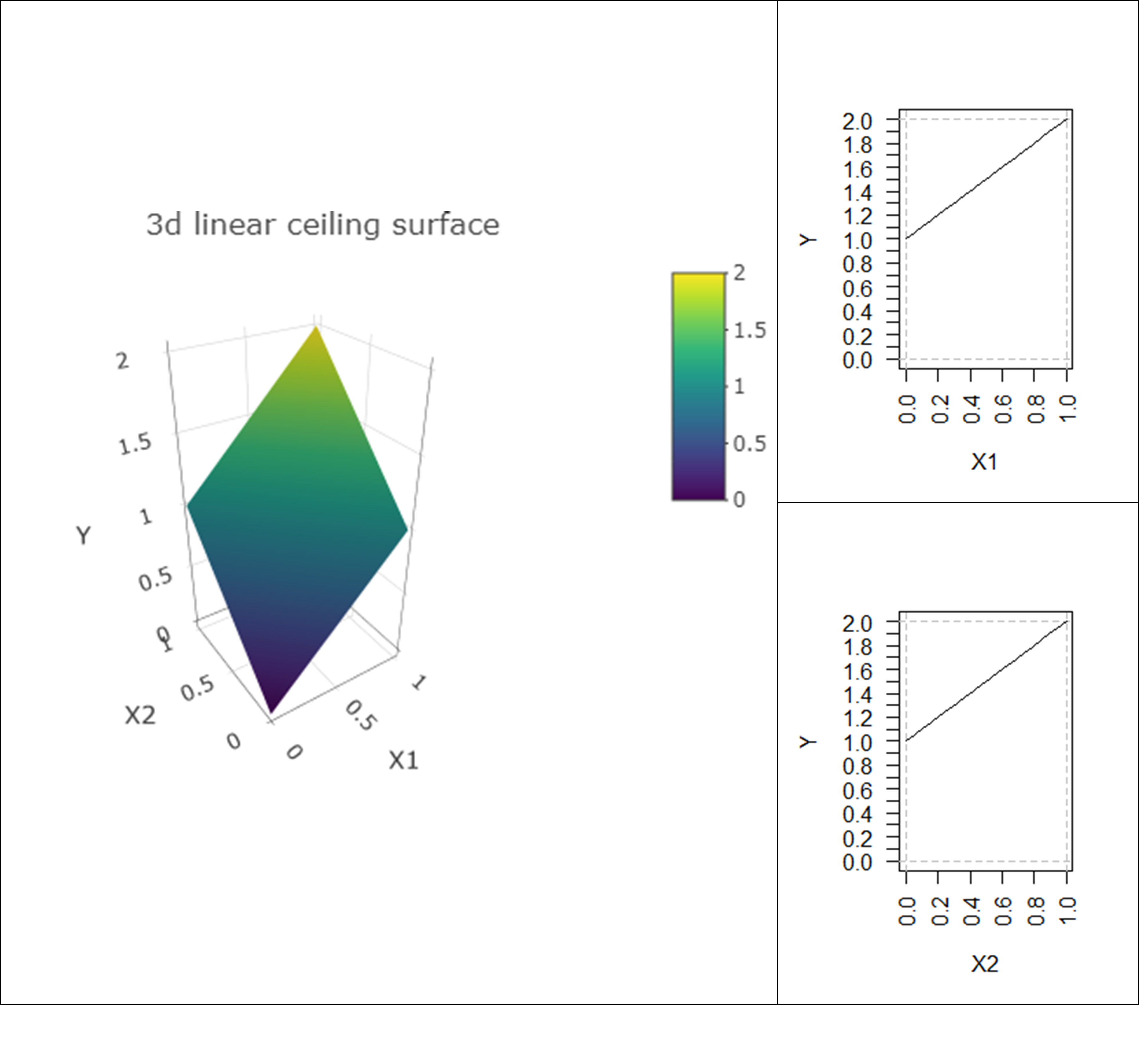
Figure 5.2: A linear multivariate three-dimensional ceiling (\(Y = X_1 + X_2\)) and its projection on the two two-dimensional \(XY\) planes (ceiling lines in \(X_1Y\) plane and in \(X_2Y\) plane).
Figure 5.3 shows a general three-dimensional non-linear ceiling surface (‘the surface of a vulcano mountain’). The projections of the surface on the \(XY\) planes result in a non-linear ceiling lines.
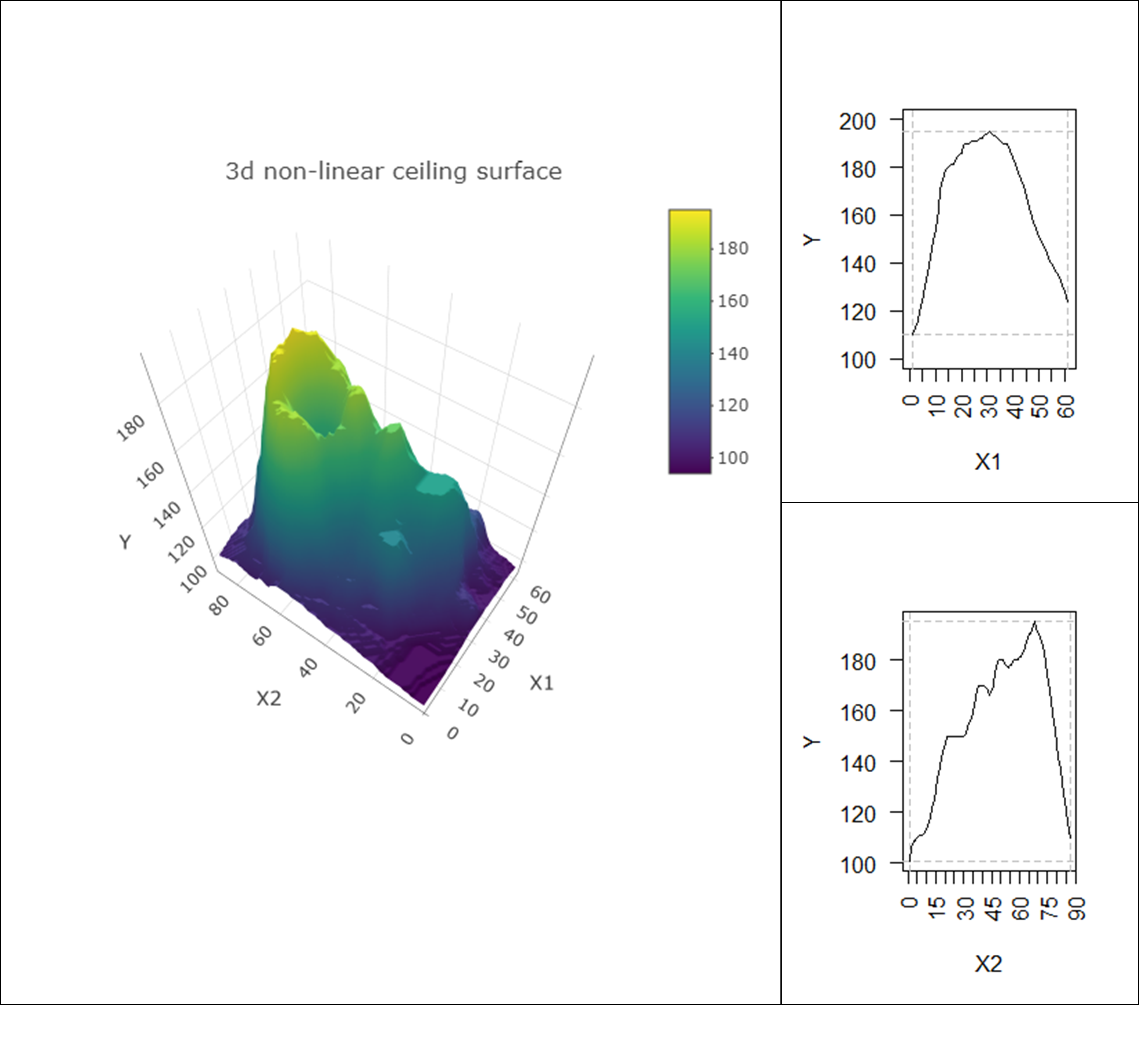
Figure 5.3: A nonlinear three-dimensional ceiling (mountain surface) and its projection (“shadow”) on two two-dimensional \(XY\) planes (non-linear ceiling lines).