Chapter 7 Miscellaneous
7.1 NCA software
7.1.1 Main NCA software: R package
The main NCA software is a free package in R called NCA(Dul & Buijs, 2023).The first version of this software was released in 2015 just before the online publication of NCA’s core paper (Dul, 2016b) on 15 July, 2015. Since then the software was updated several times to correct bugs, integrate new NCA developments, and make improvements based on feedback from users.
The following versions have been released so far:
NCA_1.0 (2015-07-02)
NCA_1.1 (2015-10-10)
NCA_2.0 (2016-05-18)
NCA_3.0 (2018-08-01)
NCA_3.0.1 (2018-08-21)
NCA_3.0.2 (2019-11-22)
NCA_3.0.3 (2020-06-11)
NCA_3.1.0 (2021-03-02)
NCA_3.1.1 (2021-05-03)
NCA_3.2.0 (2022-04-05)
NCA_3.2.1 (2022-09-15)
NCA_3.3.0 (2023-02-06)
NCA_3.3.1 (2023-02-10)
NCA_3.3.2 (2023-06-27)
NCA_3.3.3 (2023-09-05)
NCA_4.0.0 (2024-02-16)
NCA_4.0.1 (2024-02-23)
NCA_4.0.2 (2024-11-09)
When the first digit of the version number increases, major changes were implemented. Version 1 was the first limited version, version 2 was the first comprehensive version, version 3 includes the statistical test for NCA, and version 4 introduced two new functions nca_random and nca_power. The second digit refers to larger changes and the third digit minor changes.
The currently installed version of the NCA software and the availability of a new version can be checked as follows:
The cumulative number of downloads of the NCA software from the CRAN website are shown in Figure 7.1.
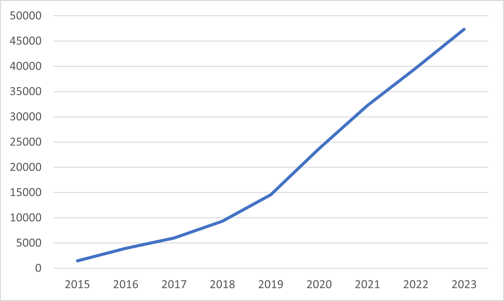
Figure 7.1: Cumulative number of downloads from the CRAN website of the NCA software since its launch).
Until 31 December 2024 the software was downloaded more than 57,000 times.
The current cumulative number of downloads can be obtained by:
library("cranlogs")
x <- cran_downloads(packages = "NCA", from = "2015-07-02", to = Sys.Date())
cat("total downloads on")
## total downloads on## [1] "2025-12-17"## [1] 69465The Quick Start Guide
(also here)
helps novice users of R and NCA to get started, but the guide also includes more advanced features. The NCA package has a build-in help function with examples. Within R, the help function can be called as follows:
When help is needed for a specific function in NCA, for example nca_analysis the help for this function can be called as follows:
7.1.2 Other NCA software packages
Based on the R package a Stata module is available for conducting NCA (Spinelli et al., 2023). NCA is also part of the SmartPLS software for conducting NCA in combination with PLS-SEM (SmartPLS Development Team, 2023). These versions enable conducting a basic NCA in other software environments than R, but lack more advanced functions and recent developments of NCA. Currently, no NCA software is available for other platforms like SPSS or SAS.
7.2 Learning about NCA
Several possibilities exist to learn about NCA. Apart from reading books and publications about the NCA methodology (Table 0.2) and reading publications with examples of NCA applications (Table 0.1) several on site and online courses are available at the introduction and advanced levels. Major international conferences often host a professional development workshop on site to learn about NCA. An example is annual conference of the the Academy of Management. Also online short introduction courses exist for NCA. An example is a free on-demand introduction seminar hosted by Instats. A longer free introduction MOOC course is available from Coursera. At the advanced level, an on-demand course is hosted by Instats. Also an NCA paper development workshop is regularly organized. More information about NCA training and events can be found in the NCA website.
7.3 Producing high-quality NCA scatter plots
One of the primary results of NCA is the ‘NCA plot’, which is a scatter plot with ceiling line(s). Users often wish to save a high quality NCA plot for further use, for example for a publication. There are several ways to make and save a high quality NCA plot. In this section six ways are presented that have different levels of user flexibility:
Standard plot.
Standard plot with basic adaptations.
Standard plot with advanced adaptations.
Advanced plot with
plotly.Advanced plot with
ggplot.From within R script.
7.3.1 Standard plot
When NCA for R is used with RStudio, the standard NCA plot is displayed in the Plots window of RStudio. The plot can be produced with the argument plots = TRUE of the nca_output function. For the example dataset in NCA package, the standard plot can be obtained as follows:
library (NCA)
data(nca.example)
model <- nca_analysis(nca.example, 1, 3)
nca_output(model, plots = TRUE, summaries = FALSE)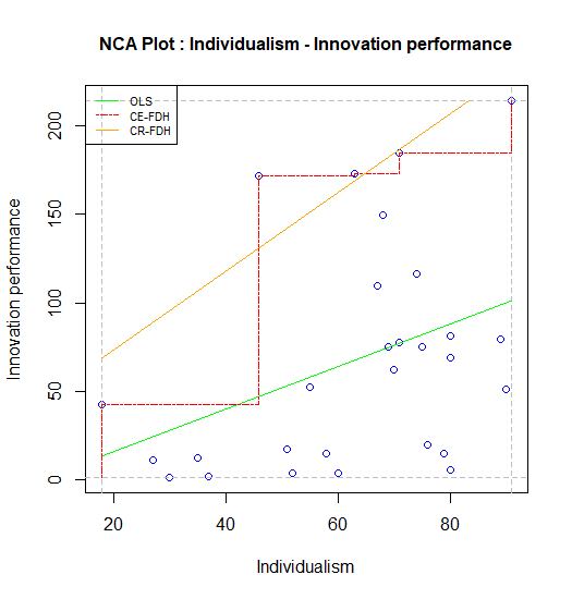
Figure 7.2: Standard scatter plot of nca.example.
7.3.2 Standard plot with basic adaptations
It may be desirable to change the appearance of the plot, such as the color of the points and the lines, the type of lines and the type of points. These characteristics can be changed with the graphical functions that are included in the NCA software. Before running nca_output, the NCA plot can be customized by changing the point type (for all points), the line types and line colors (for each ceiling line separately) and the line width (for all ceiling lines). For instance, a publisher may require a black and white or grayscale plot, with thicker lines and with solid points. Then the standard plot can be adapted as follows (changing of plot dimensions and the saving the plot is the same as for the standard plot):
line.colors['ce_fdh'] <- 'black'
line.colors['cr_fdh'] <- 'black'
line.colors['ols'] <- 'grey'
point.color <- "black"
point.type <- 20
line.width <- 2
nca_output(model, plots = TRUE, summaries = FALSE)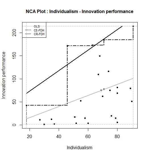
Figure 7.3: Standard scatter plot of nca.example in black/grey/white.
7.3.3 Standard plot with advanced adaptations
If further changes in the plot are needed, for example changes of the individual line types or the plot title, a special R script must be downloaded from:
https://raw.githubusercontent.com/eur-rsm/nca_scripts/master/display_plot.R
This script is used as an alternative for making the NCA plot with plots = TRUE in the nca_output function. The script can be copy/paste or otherwise loaded in your R session.
# Default values copied from p_constants
line_colors <- list(ols="green",        lh="red3",            cols="darkgreen",
                    qr="blue",          ce_vrs="orchid4",     cr_vrs="violet",
                    ce_fdh="red",       cr_fdh="orange",      sfa="darkgoldenrod",
                    c_lp="blue")
line_types  <- list(ols=3,              lh=2,                 cols=3,
                    qr=4,               ce_vrs=5,             cr_vrs=1,
                    ce_fdh=6,           cr_fdh=1,             sfa=7,
                    c_lp=2)
line_width  <- 1.5
point_type  <- 23
point_color <- 'red'
display_plot <-
  function (plot) {
    flip.x <- plot$flip.x
    flip.y <- plot$flip.y
    # Determine the bounds of the plot based on the scope
    xlim <- c(plot$scope.theo[1 + flip.x], plot$scope.theo[2 - flip.x])
    ylim <- c(plot$scope.theo[3 + flip.y], plot$scope.theo[4 - flip.y])
    # Reset/append colors etc. if needed
    for (method in names(line_types)) {
      line.types[[method]] <- line_types[[method]]
    }
    if (is.numeric(line_width)) {
      line.width <- line_width
    }
    if (is.numeric(point_type)) {
      point.type <- point_type
    }
    if (point_color %in% colors()) {
      point.color <- point_color
    }
    # Only needed until the next release (3.0.2)
    if (!exists("point.color")) {
      point.color <- "blue"
    }
    # Plot the data points
    plot (plot$x, plot$y, pch=point.type, col=point.color, bg=point.color,
          xlim=xlim, ylim=ylim, xlab=colnames(plot$x), ylab=tail(plot$names, n=1))
    # Plot the scope outline
    abline(v=plot$scope.theo[1], lty=2, col="grey")
    abline(v=plot$scope.theo[2], lty=2, col="grey")
    abline(h=plot$scope.theo[3], lty=2, col="grey")
    abline(h=plot$scope.theo[4], lty=2, col="grey")
    # Plot the legend before adding the clipping area
    legendParams = list()
    for (method in plot$methods) {
      line.color <- line.colors[[method]]
      line.type  <- line.types[[method]]
      name <- gsub("_", "-", toupper(method))
      legendParams$names  = append(legendParams$names, name)
      legendParams$types  = append(legendParams$types, line.type)
      legendParams$colors = append(legendParams$colors, line.color)
    }
    if (length(legendParams) > 0) {
      legend("topleft", cex=0.7, legendParams$names,
             lty=legendParams$types, col=legendParams$colors, bg=NA)
    }
    # Apply clipping to the lines
    clip(xlim[1], xlim[2], ylim[1], ylim[2])
    # Plot the lines
    for (method in plot$methods) {
      line <- plot$lines[[method]]
      line.color <- line.colors[[method]]
      line.type  <- line.types[[method]]
      if (method %in% c("lh", "ce_vrs", "ce_fdh")) {
        lines(line[[1]], line[[2]], type="l",
              lty=line.type, col=line.color, lwd=line.width)
      } else {
        abline(line, lty=line.type, col=line.color, lwd=line.width)
      }
    }
    # Plot the title
    title(paste0("Advanced Standard NCA Plot : ", plot$title), cex.main=1)
  }
The different default values of the plot can be changed as desired. For example, a researcher may wish to change the ols line into a dotted line (line.type to value 3), and to have a point type that is squared (point.type = 23) with red color of the points (point.color = 'red'). Also, the title of the plot can be changed at the end of the script into for example “Advanced NCA plot …”.
For producing the plot the final call is :
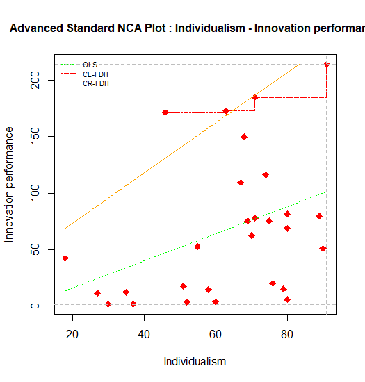
Figure 7.4: Standard scatter plot of nca.example with advance adaptations.
The plot can be reset to default values by:
7.3.4 Plot with plotly
The NCA software can also produce a plot made by plotly. The main goal is to provide the user a possibility for graphical exploration of NCA results. However, it is also possible to save the plot. The plot with plotly can be produced with the nca_output function as follows:.
It is possible to label subgroups of points. For example, the continents of the countries in the nca.example dataset can be identified as follows (in the order of the rows in the dataset):
labels <- c("Australia", "Europe", "Europe", "North America", "Europe", "Europe", "Europe", "Europe", "Europe", "Europe", "Europe", "Europe", "Europe", "Asia", "North America", "Europe", "Australia", "Europe", "Europe", "Europe", "Europe", "Asia", "Europe", "Europe", "Europe", "Europe", "Europe", "North America")
nca_output(model, plotly=labels, summaries = FALSE)
The plot opens in the Viewer tab of the plots window (Figure 7.5). The interactive version can be approached here. The plot identifies the ‘peers’ in red. Peers are points near the ceiling line that are used for drawing the default and other ceiling lines. When moving in the computer screen the pointer over the top of the plot, a toolbar pops up. One of its functions is “Download plot as png”, which saves the plot in the download folder of the computer (not in the working directory). Saving is also possible with Export tab -> Save as Image.
.](Plotly.png)
Figure 7.5: Plotly scatter plot of nca.example. The interactive version can be approached here.
7.3.5 Plot with ggplot
The function ggplot is an advanced graphical function in R. Output of NCA can be used as input for ggplot. For example, when the ceiling line is a straight line (such as the default ceiling line cr_fdh) the intercept and slope of the ceiling line can be used in ggplot to plot the ceiling line.
First, these NCA parameters must be extracted from the NCA results:
intercept <- model$summaries$Individualism$params["Intercept","cr_fdh"]
slope <- model$summaries$Individualism$params["Slope", "cr_fdh"]
Next the ggplot can be produced:
library (ggplot2)
ggplot(nca.example, aes(Individualism,`Innovation performance`))+
  geom_point() +
  geom_abline(intercept=intercept, slope=slope, col = "red")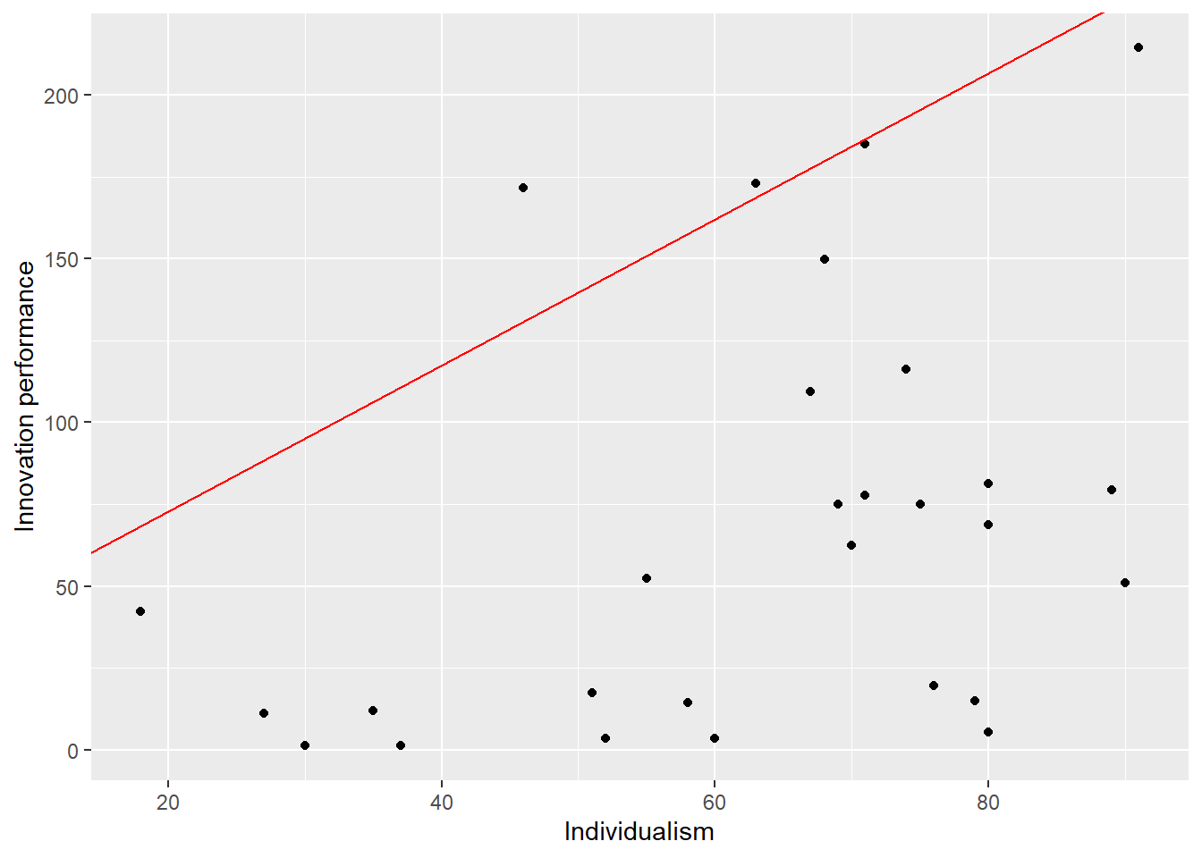
Figure 7.6: ggplot scatter plot of nca.example.
The ggplot function gives many graphical opportunities (see its documentation) to make the plot as desired.
Changing of plot dimensions and the saving the plot is the same as for the standard plot.
7.3.6 Saving the plot from within the R script
All above options for saving an NCA plot are based on first displaying the plot in R and then saving it. It is also possible to save the plot from within the R script. The following script saves a standard NCA plot as a png file with the name “nca.example.png”) in the working directory with a given size and resolution:
png("nca_example.png",units="cm", 15,15, res=300)
nca_output(model, plots = TRUE, summaries = FALSE)
dev.off()
It is also possible to save a pdf file:
7.4 Additional functions for use with the NCA softare in R (beta)
7.4.1 nca_robustness_table_general.R
# Helper function to produce the general robustness table

nca_robustness_table_general <- function(data,
                                      conditions,
                                      outcome,
                                      ceiling = "ce_fdh",
                                      scope = NULL,
                                      d_threshold = 0.1,
                                      p_threshold = 0.05,
                                      outliers = 0,
                                      bottleneck.y = "percentile",
                                      target_outcome = 75,
                                      plots = FALSE,
                                      checks = checks
) {

  # Define the configurations for each robustness check


  # Initialize an empty list to store results
  results_list <- list()

  # Perform each robustness check
  for (check in checks) {
    result <- nca_robustness_checks_general(
      data = data,
      conditions = conditions,
      outcome = outcome,
      ceiling = check$ceiling,
      scope = check$scope,
      d_threshold = check$d_threshold,
      p_threshold = check$p_threshold,
      outliers = check$outliers,
      bottleneck.y = bottleneck.y,
      target_outcome = check$target_outcome,
      plots = plots
    )
    result$`Robustness check` <- check$name
    results_list[[check$name]] <- result
  }

  # Combine all results into one data frame
  results_all <- do.call(rbind, results_list)

  # Reorder columns
  results_all <- results_all[c("Condition", "Robustness check", "Effect_size", "p_value", "Necessity", "Bottlenecks_percent", "Bottlenecks_count")]
  row.names(results_all) = NULL

  # Reorganize the dataframe into new blocks (one block per condition)
  n <- length(conditions) # Block size
  rows_per_block <- seq(1, n) # Sequence of row indices in one block

  # Create a new column to assign new block numbers
  results_all$NewBlock <- rep(rows_per_block, length.out = nrow(results_all))

  # Split the dataframe into blocks and combine the blocks sequentially
  reorganized_df <- do.call(rbind, lapply(rows_per_block, function(i) {
    results_all[results_all$NewBlock == i, ] # Subset rows for the current block
  }))

  # Remove the helper column and reset row names
  reorganized_df <- reorganized_df[, -ncol(reorganized_df)]
  row.names(reorganized_df) <- NULL
  robustness_table_general <- reorganized_df
  return(robustness_table_general)
}
7.4.2 nca_robustness_checks_general.R
# Helper function to conduct general robustness checks

nca_robustness_checks_general <- function(data,
                           conditions,
                           outcome,
                           ceiling = "ce_fdh",
                           d_threshold = 0.1,
                           p_threshold = 0.05,
                           scope = NULL,
                           outliers = 0,
                           bottleneck.y = "percentile",
                           target_outcome = 75,
                           plots = FALSE) {

  # Remove outliers if needed
  if (outliers != 0) {
    source("get_outliers.R")
    out <- get_outliers(data, conditions, outcome, ceiling, outliers)
    all_outliers <- unname(unlist(out$outliers_df)[!is.na(out$outliers_df)])
    data <- data[-all_outliers, ]
  }

  # Run the NCA analysis
  model <- nca_analysis(
    data,
    conditions,
    outcome,
    ceilings = ceiling,
    bottleneck.x = 'percentile',
    bottleneck.y = bottleneck.y,
    steps = c(target_outcome, NA),
    test.rep = 1000,
    scope = scope
  )

  # View scatter plots
  if (plots) {
  nca_output(model, summaries = FALSE) #add pdf=plots to save pdf scatter plots
  }

  # Extract effect size and p value
  effect_size <- sapply(conditions, function(e) model$summaries[[e]][[2]][[2]])
  p_value <- sapply(conditions, function(p) model$summaries[[p]][[2]][[6]])
  necessity <- ifelse(effect_size >= d_threshold & p_value <= p_threshold, "yes", "no")

  # Extract the bottlenecks data frame from the model
  b <- as.data.frame(model$bottlenecks[[1]])
  row_index <- which(b[[1]] == target_outcome)
  row_values <- b[row_index, -1]
  Bottlenecks1 <- as.numeric(row_values) # percentage bottleneck cases
  Bottlenecks2 <- round(Bottlenecks1 * nrow(data) / 100) # number bottleneck cases

  # Dataframe results
  results_all <- data.frame(
    Condition = conditions,
    Effect_size = effect_size,
    p_value = p_value,
    Necessity = necessity,
    Bottlenecks_percent = Bottlenecks1,
    Bottlenecks_count = Bottlenecks2
  )

  return(results_all)
}
7.4.3 get_outliers.R
# Helper function to get outliers
# Revised June 1, 2025

get_outliers <- function (data, conditions, outcome, ceiling, k, row.numbers = TRUE) {
  if (row.numbers) {
    rownames(data) <- NULL
  }

  # Apply nca_outliers for each condition in the conditions vector
  outliers_list <- lapply(conditions, function (condition) {
    nca_outliers(data, x = condition, y = outcome, ceiling = ceiling, k = k)
  })

  # Extract the k datapoints for the first outlier, add NA's if needed
  k_outliers <- lapply(outliers_list, function(o) {
    # Check if o is a valid list/matrix and has a non-NULL, non-NA string in position [1,1]
    if (is.null(o) || is.null(o[[1, 1]]) || is.na(o[[1, 1]]) || !is.character(o[[1, 1]])) {
      return(rep(NA, k))
    }

    parts <- unlist(strsplit(o[[1, 1]], " - ", fixed = TRUE))
    if (row.numbers) {
      parts <- as.numeric(parts)
    }
    c(parts, rep(NA, k - length(parts)))
  })

  outliers_df <- do.call(rbind, k_outliers)
  colnames(outliers_df) <- paste("Outlier", 1:k)
  rownames(outliers_df) <- conditions

  return(list(outliers_list = outliers_list, outliers_df = outliers_df))
}
7.4.4 get_indicator_data_TAM.R
# Helper function for getting indicator data of TAM example
#revised May 23, 2025

# Literature:
# Hauff, S., Richter, N. F., Sarstedt, M., & Ringle, C. M. (2024).
# Importance and performance in PLS-SEM and NCA: Introducing the combined importance-performance map analysis (cIPMA).
# Journal of Retailing and Consumer Services, 78, 103723.
# https://doi.org/10.1016/j.jretconser.2024.103723

# Richter, N. F., Schubring, S., Hauff, S., Ringle, C. M., & Sarstedt, M. (2020).
# When predictors of outcomes are necessary: Guidelines for the combined use of PLS-SEM and NCA.
# Industrial Management & Data Systems, 120(12), 2243–2267.
# https://doi.org/10.1108/IMDS-11-2019-0638

# Richter, N. F., Hauff, S., Ringle, C. M., Sarstedt, M., Kolev, A. E., & Schubring, S. (2023).
# How to apply necessary condition analysis in PLS-SEM. In Partial least squares path modeling: Basic concepts, methodological issues and applications (pp. 267–297).
# Springer.
# https://link.springer.com/chapter/10.1007/978-3-031-37772-3_10

# Sarstedt, M., Richter, N. F., Hauff, S., & Ringle, C. M. (2024).
# Combined importance–performance map analysis (cIPMA) in partial least squares structural equation modeling (PLS–SEM): A SmartPLS 4 tutorial.
# Journal of Marketing Analytics, 1–15.
# https://doi.org/10.1057/s41270-024-00325-y

# Data sources:
# Schubring, S., & Richter, N. (2023).
# Extended TAM (Version V4).
# Mendeley Data.
# https://doi.org/10.17632/pd5dp3phx2.4https://osf.io/35a6d/files/osfstorage?view_only=849040255d43480696cd60a43d664660

# Richter, N. F., Hauff, S., Kolev, A. E., & Schubring, S. (2023).
# Dataset on an extended technology acceptance model: A combined application of PLS-SEM and NCA.
# Data in Brief, 48, 109190.
# https://doi.org/10.1016/j.dib.2023.109190

get_indicator_data_TAM <- function(){

# Load the data
df0 <- read.csv("Extended TAM.csv")

# Preview the data
head(df0, 3)

# Make a new dataset with only indicator scores of SEM model (without last four variables)
df1 <- df0[, 1:(ncol(df0) - 4)]

# Rename the indicators
colnames(df1) <- c("PU1","PU2","PU3",
                   "CO1","CO2","CO3",
                   "EOU1", "EOU2","EOU3",
                   "EMV1", "EMV2","EMV3",
                   "AD1",  "AD2","AD3",
                   "USE")

# Preview the new dataset
head(df1,3)

return(df1)
}
7.4.5 estimate_sem_model_TAM.R
# Helper function to estimate SEM model for the TAM example
# revised 23 May, 2025

estimate_sem_model_TAM <- function(data){
# Load library for conducting SEM
library(seminr)

# Specify the measurement model
TAM_mm <- constructs(
  composite("Perceived usefulness", multi_items("PU", 1:3)),
  composite("Compatibility", multi_items("CO", 1:3)),
  composite("Perceived ease of use", multi_items("EOU", 1:3)),
  composite("Emotional value", multi_items("EMV", 1:3)),
  composite("Adoption intention", multi_items("AD", 1:3)),
  composite("Technology use", single_item("USE"))
)

# Specify the structural model
TAM_sm <- relationships(
  paths(from = "Perceived usefulness", to = c("Adoption intention", "Technology use")),
  paths(from = "Compatibility",         to = c("Adoption intention", "Technology use")),
  paths(from = "Perceived ease of use", to = c("Adoption intention", "Technology use")),
  paths(from = "Emotional value",       to = c("Adoption intention", "Technology use")),
  paths(from = "Adoption intention",    to = c("Technology use"))
)

# Estimate the pls model (using indicator data)

# Conduct pls estimation with raw indicator scores
TAM_pls <- estimate_pls(data = data,
                        measurement_model = TAM_mm,
                        structural_model = TAM_sm)

# Print path coefficients and model fit measures
summary(TAM_pls)

return (TAM_pls)
}
7.4.6 get_signficance_sem.R
# Helper function to get significance of SEM predictors
# Revised August 4, 2025

get_significance_sem <- function(sem, nboot = 5000) {

  # Run bootstrap
  boot_model <- bootstrap_model(sem, nboot = nboot) # alpha is fixed at 0.05

  # Extract direct and total path matrices
  df_direct <- as.data.frame(summary(boot_model)[[2]])
  df_total  <- as.data.frame(summary(boot_model)[[6]])

  # Rename confidence interval columns
  colnames(df_direct)[5:6] <- c("CI_low", "CI_high")
  colnames(df_total)[5:6]  <- c("CI_low", "CI_high")

  # Add Path column from rownames
  df_direct <- cbind(Path = rownames(df_direct), df_direct)
  df_total  <- cbind(Path = rownames(df_total), df_total)

  # Reset row names
  rownames(df_direct) <- NULL
  rownames(df_total)  <- NULL

  # Keep original order
  path_order <- df_direct$Path

  # Merge direct and total
  merged_df <- merge(df_total, df_direct, by = "Path", suffixes = c("_total", "_direct"))

  # Clean column names for safe access
  colnames(merged_df) <- make.names(colnames(merged_df))

  # Calculate indirect effect
  merged_df$Indirect_Estimate <- merged_df$Original.Est._total - merged_df$Original.Est._direct

  # Significance flags
  merged_df$Sig_Direct   <- (merged_df$CI_low_direct > 0 | merged_df$CI_high_direct < 0)
  merged_df$Sig_Total    <- (merged_df$CI_low_total > 0 | merged_df$CI_high_total < 0)
  merged_df$Sig_Indirect <- merged_df$Sig_Total & !merged_df$Sig_Direct

  # Final summary
  summary_df <- merged_df[, c(
    "Path",
    "Original.Est._direct", "Indirect_Estimate", "Original.Est._total",
    "Sig_Direct", "Sig_Indirect", "Sig_Total"
  )]

  # Round for readability
  summary_df <- within(summary_df, {
    Original.Est._direct  <- round(Original.Est._direct, 3)
    Indirect_Estimate     <- round(Indirect_Estimate, 3)
    Original.Est._total   <- round(Original.Est._total, 3)
  })

  # Preserve original order
  summary_df$Path <- factor(summary_df$Path, levels = path_order)
  summary_df <- summary_df[order(summary_df$Path), ]

  colnames(summary_df)[2:4] <- c("Direct", "Indirect", "Total")

  # Extract predicted variable from path (RHS of arrow)
  get_rhs <- function(path_string) {
    strsplit(as.character(path_string), "->")[[1]][2] |> trimws()
  }
  summary_df$Predicted <- sapply(as.character(summary_df$Path), get_rhs)

  # Return final table
  return(summary_df)
}
7.4.7 unstandardize.R
# Helper function to obtain a dataset with the unstandardized latent variables
# using the output of the SEMinR pls model estimation as function argument.

# Revised May 23, 2025
unstandardize <- function(sem) {

  # Extract the original indicators
  original_indicators_df <- as.data.frame(sem$rawdata)

  # Extract the standardized weights and store results in a dataframe
  standardized_weights_matrix <- sem$outer_weights
  standardized_weights_df <- as.data.frame(as.table(standardized_weights_matrix))
  colnames(standardized_weights_df) <- c("Indicator", "Latent variable", "Standardized weight")
  standardized_weights_df <- subset(standardized_weights_df, `Standardized weight` != 0)

  # Match SDs to indicators
  standardized_weights_df$SD <- sem$sdData[as.character(standardized_weights_df$Indicator)]

  # Compute unstandardized weights
  standardized_weights_df$`Unstandardized weight` <-
  standardized_weights_df$`Standardized weight` / standardized_weights_df$SD  # Following Ringle and Sarstedt 2016

   # Normalize weights within each latent variable
  sum_weights <- tapply(
    standardized_weights_df$`Unstandardized weight`,
    standardized_weights_df$`Latent variable`,
    sum
  )

  standardized_weights_df$`Sum unstandardized weight` <-
    sum_weights[match(standardized_weights_df$`Latent variable`, names(sum_weights))]

  standardized_weights_df$`Normalized unstandardized weight` <-
    standardized_weights_df$`Unstandardized weight` / standardized_weights_df$`Sum unstandardized weight`

  # Compute unstandardized latent variables
  unstandardized_latent_variable_df <- data.frame(matrix(nrow = nrow(original_indicators_df), ncol = 0))

  for (latent_variable in unique(standardized_weights_df$`Latent variable`)) {
    latent_data <- subset(standardized_weights_df, `Latent variable` == latent_variable)
    indicators <- as.character(latent_data$Indicator)
    weights <- latent_data$`Normalized unstandardized weight`
    indicator_scores <- original_indicators_df[, indicators, drop = FALSE]
    latent_score <- rowSums(sweep(indicator_scores, 2, weights, `*`))
    unstandardized_latent_variable_df[[latent_variable]] <- latent_score
  }

  return(unstandardized_latent_variable_df)
}
7.4.8 normalize.R
# Helper function to min-max normalize data (scale 0-1 or 0-100)
# Revised August 9, 2025

min_max_normalize <- function(data, theoretical_min, theoretical_max, scale) {

  # Validate inputs
  if (!is.numeric(scale) || length(scale) != 2) {
    stop("Scale must be a numeric vector with two elements (e.g., c(0, 100)).")
  }

  if (!is.numeric(theoretical_min) || !is.numeric(theoretical_max)) {
    stop("Theoretical min and max must be numeric vectors.")
  }

  # Define new scale minimum and maximum
  new_min <- scale[1]
  new_max <- scale[2]

  # Apply normalization column by column
  normalized_data <- data
  for (i in seq_along(data)) {
    if (is.numeric(data[[i]])) {
      min_val <- theoretical_min[i]
      max_val <- theoretical_max[i]

      # Standard normalization
      norm_values <- ((data[[i]] - min_val) / (max_val - min_val)) *
        (new_max - new_min) + new_min

      # avoid floating-point error
      tol <- sqrt(.Machine$double.eps) * abs(new_max - new_min)
      if (new_min == 0) norm_values[data[[i]] == 0] <- 0  # optional: preserve exact zeros
      norm_values[abs(norm_values - new_min) < tol] <- new_min
      norm_values[abs(norm_values - new_max) < tol] <- new_max
      norm_values <- pmax(new_min, pmin(new_max, norm_values))

      normalized_data[[i]] <- norm_values
    }
  }

  # Return the normalized dataframe
  return(normalized_data)
}
7.4.9 get_bottleneck_cases.R
# Helper function to find the number and percentage of bottleneck cases per condition
#revised August 10, 2025

get_bottleneck_cases <- function(data, conditions, outcome, corner = 1, target_outcome, ceiling) {
  # Check if target_outcome is within the range of the outcome variable
  outcome_min <- min(data[[outcome]], na.rm = TRUE)
  outcome_max <- max(data[[outcome]], na.rm = TRUE)

  if (length(corner) == 1 && corner == 1) {corner <- rep(1, length(conditions))}

  if (target_outcome < outcome_min || target_outcome > outcome_max) {
    stop(
      sprintf(
        "Error: target_outcome (%f) is out of range for the outcome variable '%s'. Minimum: %f, Maximum: %f",
        target_outcome, outcome, outcome_min, outcome_max
      )
    )
  }

  # Initialize matrices to store bottlenecks
  bottleneck_matrix <- matrix(0, nrow = nrow(data), ncol = length(conditions))
  colnames(bottleneck_matrix) <- conditions

  threshold <- setNames(numeric(length(conditions)), conditions)
  eps <- .Machine$double.eps^0.5  # Smallest safe numerical tolerance

  for (condition in conditions) {
    # Find index of the condition
    condition_index <- which(conditions == condition)[1]  # Get the index of the current condition

    # Get corner value
    corner_val <- corner[condition_index]

    # Check if corner_val is NA or not in valid range (1 to 4)
    if (is.na(corner_val)) {
      warning(sprintf("Warning: corner value for condition '%s' is NA. Defaulting to 1.", condition))
      corner_val <- 1L
    } else if (!(corner_val %in% 1:4)) {
      warning(sprintf("Warning: corner value for condition '%s' (%d) is out of valid range (1-4). Defaulting to 1.", condition, corner_val))
      corner_val <- 1L
    }

    # Perform NCA for the given condition
    model1 <- nca_analysis(
      data,
      condition,
      outcome,
      corner = corner_val,
      ceilings = ceiling,
      bottleneck.y = "actual",
      bottleneck.x = "actual",
      steps = c(target_outcome, NA)
    )
    # Extract accurate threshold
      threshold[condition] <- attr(model1[["bottlenecks"]][[ceiling]][[condition]],"mpx.actual")[1, 1]

      if (corner_val %in% c(1, 3)) {
        bottleneck_matrix[, condition] <- as.numeric(
          data[[condition]] < (threshold[condition] - eps)
        )
      } else {
        bottleneck_matrix[, condition] <- as.numeric(
          data[[condition]] > (threshold[condition] - eps)
        )
      }

    # If no cases are bottlenecks, reset to 0
      if (sum(bottleneck_matrix[, condition]) == nrow(data)) {
        bottleneck_matrix[, condition] <- 0
      }
      if (threshold[condition] == -Inf) {
        threshold[condition] <- 0
      }
  }

  # Calculate the total bottlenecks for each column
  bottlenecks_per_condition <- colSums(bottleneck_matrix)
  bottleneck_cases_num <- as.data.frame (bottlenecks_per_condition) # number
  colnames(bottleneck_cases_num)[1] <- paste0("Bottlenecks (Y = ", target_outcome, ")")
  bottleneck_cases_per <- as.data.frame (100 * (bottleneck_cases_num / nrow(data))) # percentage

  return(list(
    bottleneck_cases_per = bottleneck_cases_per,
    bottleneck_cases_num = bottleneck_cases_num
  ))

}
7.4.10 get_ipma_df.R
# Helper function to create an IPMA dataset with Importance and Performance
# Revised Aug 8, 2025 - includes inversion handling for negative importance

get_ipma_df <- function(data, sem, predictors, predicted) {

  # Importance = total effects
  Importance_df <- as.data.frame(summary(sem)$total_effects)
  Importance <- Importance_df[predictors, predicted]

  # Performance = means of all latent variable scores
  Performance_df <- as.data.frame(sapply(data, mean))
  Performance <- Performance_df[predictors, 1]

  # Invert names and take absolute values where importance is negative
  renamed_predictors <- ifelse(Importance < 0,
                               paste0(predictors, "-inv"),
                               predictors)
  Importance <- abs(Importance)

  # Combine into IPMA dataframe
  ipma_df <- data.frame(
    predictor = renamed_predictors,
    Importance = Importance,
    Performance = Performance
  )

  return(ipma_df)
}
7.4.11 get_ipma_plot.R
# Helper function to create a IPMA plot
# Revised May 23, 2025

# Load required libraries
library(ggplot2)
library(ggrepel)

get_ipma_plot <- function(ipma_df,
                          x_range = NULL,
                          y_range = NULL) {

  # Dynamically set x_range if not provided
  if (is.null(x_range)) {
    x_range <- range(ipma_df$Importance, na.rm = TRUE)
  }

  # Dynamically set y_range if not provided
  if (is.null(y_range)) {
    y_range <- range(ipma_df$Performance, na.rm = TRUE)
  }

  # Generate the IPMA plot
  p <- ggplot(ipma_df, aes(x = Importance, y = Performance)) +
    geom_point(color = "black", size = 5) +  # Single point layer
    geom_text_repel(
      aes(label = predictor),
      size = 3.5,
      box.padding = 2
    ) +
    coord_cartesian(xlim = x_range, ylim = y_range) +
    scale_x_continuous(limits = x_range) +  # Adapt x-axis limits dynamically
    scale_y_continuous(limits = y_range) +  # Adapt y-axis limits dynamically
    labs(
      title = "classic IPMA",
      x = "Importance",
      y = "Performance"
    ) +
    theme_minimal()  # Use a clean theme

  # Display the plot
  print(p)
}
7.4.12 get_cipma_df.R
# Helper function to create a cIPMA dataset with Importance, Performance,
# and Bottlenecks (percentage and number of bottleneck cases)
# Revised August 9, 2025

get_cipma_df <- function(ipma_df, bottlenecks, necessity) {

  # Extract number and percentage of single bottleneck cases
  cases_num <- bottlenecks$bottleneck_cases_num
  cases_per <- bottlenecks$bottleneck_cases_per

  # Combine IPMA data with bottleneck info
  cipma_df <- cbind(
    ipma_df,
    cases_per,
    cases_num
  )
  rownames(cipma_df) <- rownames(ipma_df)
  colnames(cipma_df)[4:5] <- c("Bottleneck_cases_per", "Bottleneck_cases_num")


  # Add necessity classification
  cipma_df$Necessity <- necessity

  # Add predictor labels:
  cipma_df$Predictor_with_cases <- ifelse(
    cipma_df$Necessity == "yes",
    paste0(
      cipma_df$predictor,
      " (",
      round(cipma_df$Bottleneck_cases_per, 0), "%, n=",
      cipma_df$Bottleneck_cases_num,
      ")"
    ),
    paste0(cipma_df$predictor, " (NN)")
  )

  return(cipma_df)
}
7.4.13 get_cipma_plot.R
# Helper function for producing the cIPMA plot
# Revised August 10, 2025

get_cipma_plot <- function(cipma_df, x_range = NULL, y_range = NULL, size_limits, size_range) {

  # Load required libraries
  library(ggplot2)
  library(ggrepel)

  # Dynamically determine x_range if not provided
  if (is.null(x_range)) {
    x_range <- range(bipma_df$Importance, na.rm = TRUE)
  }

  # Dynamically determine y_range if not provided
  if (is.null(y_range)) {
    y_range <- range(bipma_df$Performance, na.rm = TRUE)
  }

  # Extract target Y value from column name
  colname <- colnames(cipma_df)[4]
  target.Y <- target_outcome

  # Set fill color: black only for NN cases
  cipma_df$fill_color <- ifelse(
    grepl("\\(NN\\)", cipma_df$Predictor_with_cases),
    "black",
    NA
  )

  # Set dot size: fixed small size for NN, scaled otherwise
  cipma_df$dot_size <- ifelse(
    grepl("\\(NN\\)", cipma_df$Predictor_with_cases),
    1,
    cipma_df[[colname]]
  )

  # Generate the plot
  pc <- ggplot(cipma_df, aes(x = Importance, y = Performance)) +
    geom_point(
      aes(size = dot_size),
      shape = 21,
      fill = cipma_df$fill_color,
      color = "black",
      stroke = 0.7
    ) +
    geom_text_repel(
      aes(label = Predictor_with_cases),
      size = 3.5,
      box.padding = 2
    ) +
    coord_cartesian(xlim = x_range, ylim = y_range) +
    scale_x_continuous(limits = x_range) +
    scale_y_continuous(limits = y_range) +
    scale_size_continuous(limits = size_limits, range = size_range) +
    labs(
      title = paste("cIPMA for target outcome Y =", target.Y, " ", name_plot),
      x = "Importance",
      y = "Performance"
    ) +
    theme_minimal() +
    guides(size = "none", fill = "none")  # REMOVE LEGEND

  # Display the plot
  print(pc)
}
7.4.14 get_single_bottleneck_cases.R
# Helper function to find the number of single bottleneck cases per condition
# Revised August 10, 2025

get_single_bottleneck_cases <- function(data, conditions, outcome, corner = 1, target_outcome, ceiling) {
  # Check if target_outcome is within the range of the outcome variable
  outcome_min <- min(data[[outcome]], na.rm = TRUE)
  outcome_max <- max(data[[outcome]], na.rm = TRUE)

  if (length(corner) == 1 && corner == 1) {corner <- rep(1, length(conditions))}

  if (target_outcome < outcome_min || target_outcome > outcome_max) {
    stop(
      sprintf(
        "Error: target_outcome (%f) is out of range for the outcome variable '%s'. Minimum: %f, Maximum: %f",
        target_outcome, outcome, outcome_min, outcome_max
      )
    )
  }

  # Initialize matrices to store bottlenecks
  bottleneck_matrix <- matrix(0, nrow = nrow(data), ncol = length(conditions))
  colnames(bottleneck_matrix) <- conditions

  threshold <- setNames(numeric(length(conditions)), conditions)
  eps <- .Machine$double.eps^0.5  # Smallest safe numerical tolerance

  for (condition in conditions) {

    # Find index of the condition
    condition_index <- which(conditions == condition)[1]  # Get the index of the current condition

    # Get corner value
    corner_val <- corner[condition_index]

    # Check if corner_val is NA or not in valid range (1 to 4)
    if (is.na(corner_val)) {
      warning(sprintf("Warning: corner value for condition '%s' is NA. Defaulting to 1.", condition))
      corner_val <- 1L
    } else if (!(corner_val %in% 1:4)) {
      warning(sprintf("Warning: corner value for condition '%s' (%d) is out of valid range (1-4). Defaulting to 1.", condition, corner_val))
      corner_val <- 1L
    }

    # Perform NCA for the given condition
    model1 <- nca_analysis(
      data,
      condition,
      outcome,
      corner = corner_val,
      ceilings = ceiling,
      bottleneck.y = "actual",
      bottleneck.x = "actual",
      steps = c(target_outcome, NA)
    )
    # Extract accurate threshold
    threshold[condition] <- attr(model1[["bottlenecks"]][[ceiling]][[condition]],"mpx.actual")[1, 1]

    if (corner_val %in% c(1, 3)) {
      bottleneck_matrix[, condition] <- as.numeric(
        data[[condition]] < (threshold[condition] - eps)
      )
    } else {
      bottleneck_matrix[, condition] <- as.numeric(
        data[[condition]] > (threshold[condition] - eps)
      )
    }

    # If no cases are bottlenecks, reset to 0
    if (sum(bottleneck_matrix[, condition]) == nrow(data)) {
      bottleneck_matrix[, condition] <- 0
    }
    if (threshold[condition] == -Inf) {
      threshold[condition] <- 0
    }
  }

  # Calculate the total bottlenecks for each row
  total_bottlenecks_per_row <- rowSums(bottleneck_matrix)

  # Count the number of rows where each case is the sole bottleneck
  single_bottlenecks_per_condition <- colSums(bottleneck_matrix & (total_bottlenecks_per_row == 1))

  single_bottleneck_cases_num <- as.data.frame (single_bottlenecks_per_condition) # number
  colnames(single_bottleneck_cases_num)[1] <- paste0("Bottlenecks (Y = ", target_outcome, ")")
  single_bottleneck_cases_per <- as.data.frame (100 * (single_bottleneck_cases_num / nrow(data))) # percentage

  return(list(
    single_bottleneck_cases_per = single_bottleneck_cases_per,
    single_bottleneck_cases_num = single_bottleneck_cases_num
  ))

}
7.4.15 get_bipma_df.R
# Helper function to create a BIPMA dataset with Importance, Performance,
# and Bottlenecks (percentage and number of SINGLE bottleneck cases)
# Revised November 8, 2025

get_bipma_df <- function(ipma_df, single_bottlenecks, necessity, sufficiency) {

  # Extract number and percentage of single bottleneck cases
  single_cases_num <- single_bottlenecks$single_bottleneck_cases_num
  single_cases_per <- single_bottlenecks$single_bottleneck_cases_per

  # Combine IPMA data with bottleneck info
    bipma_df <- cbind(
    ipma_df,
    single_cases_per,
    single_cases_num
  )

  rownames(bipma_df) <- rownames(ipma_df)
  colnames(bipma_df)[4:5] <- c("Single_bottleneck_cases_per", "Single_bottleneck_cases_num")

  # Add necessity classification
  bipma_df$Necessity <- necessity

  # Add corner classification
  bipma_df$Corner <- corner

  # Add target_outcome
  bipma_df$Target_outcome <- target_outcome

  # Add probabilistic sufficiency classification
  bipma_df$Sufficiency <- sufficiency

  # Add predictor labels:
  bipma_df$Predictor_with_single_cases <- ifelse(
    bipma_df$Necessity == "yes",
    paste0(
      bipma_df$predictor,
      " (",
      round(bipma_df$Single_bottleneck_cases_per, 0), "%, n=",
      bipma_df$Single_bottleneck_cases_num,
      ifelse(
        bipma_df$Corner %in% c(2, 3, 4),
        paste0(", corner=", bipma_df$Corner),
        ""
      ),
      ")"
    ),
    paste0(bipma_df$predictor, " (NN)")
  )

  return(bipma_df)
}
7.4.16 get_bipma_plot.R
# Helper function for producing the BIPMA plot
# Revised November 8, 2025

get_bipma_plot <- function(bipma_df, x_range = NULL, y_range = NULL, size_limits, size_range) {

  library(ggplot2)
  library(ggrepel)

  # For visibility of overlapping filled points
  bipma_df <- bipma_df[order(bipma_df$Single_bottleneck_cases_num, decreasing = TRUE), ]

  # Dynamically determine x_range if not provided
  if (is.null(x_range)) {
    x_range <- range(bipma_df$Importance, na.rm = TRUE)
  }

  # Dynamically determine y_range if not provided
  if (is.null(y_range)) {
    y_range <- range(bipma_df$Performance, na.rm = TRUE)
  }

  # Extract the bottleneck column name
  colname <- colnames(bipma_df)[4]
  target.Y <- target_outcome

  bipma_df$fill_color <- ifelse(
    grepl("\\(NN\\)", bipma_df$Predictor_with_single_cases),
    "black",
    NA_character_
  )
  bipma_df$fill_color[is.na(bipma_df$fill_color) & bipma_df$Sufficiency == "no"] <- "grey90"
  bipma_df$fill_color[is.na(bipma_df$fill_color)] <- "white"

  # Define dot size: fixed small size for NN, scaled otherwise
  bipma_df$dot_size <- ifelse(
    grepl("\\(NN\\)", bipma_df$Predictor_with_single_cases),
    1,
    bipma_df[[colname]]
  )

  # Adjust importance for plotting
  x_no <- -0.00  # x-position for "no sufficiency" predictors
  bipma_df$Importance_adj <- ifelse(
    bipma_df$Sufficiency == "no",
    x_no,
    bipma_df$Importance
  )

  # Define x-range (include the no sufficiency zone to give space for points)
  x_range_adj <- c(x_no - 0.02 , max(bipma_df$Importance, na.rm = TRUE) + 0.1)
  x_breaks <- pretty(bipma_df$Importance)

  ## 1) keep the NN & NS names BEFORE removing them
  dropped_idx <- (bipma_df$Necessity == "no" & bipma_df$Sufficiency == "no")
  dropped_names <- bipma_df$predictor[dropped_idx]

  # Remove predictors that are not necessary and not sufficient
  bipma_df <- bipma_df[!dropped_idx, ]

  # Plot
  pc1 <- ggplot(bipma_df, aes(x = Importance_adj, y = Performance)) +

    geom_point(
      aes(size = dot_size, fill = fill_color),
      shape = 21,
      color = "black",
      stroke = 0.7
    ) +
    scale_fill_identity() +

    geom_text_repel(
      aes(label = Predictor_with_single_cases),
      size = 3.5,
      box.padding = 2
    ) +

    coord_cartesian(xlim = x_range_adj, ylim = y_range) +
    scale_x_continuous(
      breaks = x_breaks,
      limits = x_range_adj
    ) +
    scale_y_continuous(limits = y_range) +
    scale_size_continuous(limits = size_limits, range = size_range) +

    labs(
      title = paste("BIPMA for target outcome Y =", target.Y, name_plot),
      x = "Importance",
      y = "Performance"
    ) +
    theme_minimal() +
    theme(
      axis.text.x = element_text(),
      axis.ticks.x = element_line(),
      panel.grid.minor = element_blank()
    ) +
    guides(size = "none")

  ## 2) add the textbox in the lower-left corner (only if there were dropped ones)
  if (length(dropped_names) > 0) {
    pc1 <- pc1 +
      annotate(
        "label",
        x = x_range_adj[1] + 0.01,     # a little inside the panel
        y = y_range[1] + 0.01,
        hjust = 0,
        vjust = 0,
        label = paste(
          c("Non-significant necessity and average effects:", dropped_names),
          collapse = "\n"
        ),
        size = 3
      )
  }
  print(pc1)
}
7.4.17 ncasem.R
# Function to conduct NCA-SEM
# Revised November 8, 2025

#Helper functions to be sourced (below):
# source("unstandardize.R")
# source("normalize.R")
# source("get_outliers.R")
# source("get_ipma_df.R")
# source("get_ipma_plot.R")
# source("get_bottleneck_cases.R")
# source("get_cipma_df.R")
# source("get_cipma_plot.R")
# source("get_single_bottleneck_cases.R")
# source("get_bipma_df.R")
# source("get_bipma_plot.R")

ncasem <- function(sem,
                   sem_sig,
                   outliers = 0,
                   standardize = 0, # unstandardized
                   normalize = 1, # normalized
                   scale = c(0,100), # normalized 0-100 (percentage)
                   predictors,
                   predicted,
                   theoretical_min,
                   theoretical_max,
                   corner = corner,
                   ceiling = "ce_fdh",
                   test.rep = test.rep,
                   d_threshold = 0.10,
                   p_threshold = 0.05,
                   scope = NULL, # empirical scope
                   target_outcome,
                   plots = FALSE,
                   name_plot = name_plot) {


  #Step 3 select latent variable scores
  data <- sem$construct_scores
  # Standardization step
  if (standardize == 0) {
    source("unstandardize.R")
    data <- unstandardize(sem)
  }

  # Normalization step
  if (normalize == 0) {
    data <- data  # No normalization
  } else {
    source("normalize.R")
    data <- min_max_normalize(data, theoretical_min, theoretical_max, scale)
  }


  # Step 4: Conduct NCA

  library(NCA)
  data <- data
  ceilings = ceiling
  corner = corner
  test.rep = test.rep #set the number of permutations for estimating the p value
  # bottleneck.y = "actual"
  # bottleneck.x = "percentile"
  # steps=seq(0, 100, 5)
  scope=scope

  # Process outliers if needed
  if (outliers != 0) {
    source("get_outliers.R")
    conditions = predictors
    outcome = predicted
    k = outliers
    out <- get_outliers(data = data,
                        conditions = conditions,
                        outcome = outcome,
                        ceiling = ceiling,
                        k = k)
    all_outliers <- unname(unlist(out$outliers_df)[!is.na(out$outliers_df)])
    # Remove outliers
    data <- data[-all_outliers, ]
  }

  # Run the NCA analysis
  model <- nca_analysis(
    data,
    predictors,
    predicted,
    corner = corner,
    ceilings = ceiling,
  #  bottleneck.x = bottleneck.x,
  #  bottleneck.y = bottleneck.y,
  #  steps = steps,
    test.rep = test.rep,
    scope = scope
  )

  nca_output(model, summaries = FALSE, pdf = plots)

  # Step 5: Produce BIPMA
  # IPMA
  source("get_ipma_df.R")
  IPMA_df <- get_ipma_df(data = data, sem = sem, predictors = predictors, predicted = predicted)
  ipma_df <- IPMA_df
  source("get_ipma_plot.R")
  IPMA_plot <- get_ipma_plot(ipma_df = ipma_df, x_range = x_range, y_range = y_range)
  if (plots) {
    current_time <- format(Sys.time(), "%Y-%m-%d_%H-%M-%S")
    filename <- paste0("IPMA plot_", current_time, ".pdf")
    ggsave(filename, plot = IPMA_plot, width = 8, height = 6, dpi = 300)
  }

  # CIPMA
  # NCA parameters
  effect_size <- sapply(predictors, function(d) model$summaries[[d]][[2]][[2]])
  p_value <- sapply(predictors, function(p) model$summaries[[p]][[2]][[6]])
  # Select predictors that are necessary
  necessity <- ifelse(effect_size >= d_threshold & p_value <= p_threshold, "yes", "no")

  #number and percentage of bottleneck cases (more accurate via loop)
  source("get_bottleneck_cases.R")
  bottlenecks <- get_bottleneck_cases(data = data, conditions = predictors, outcome = predicted, corner = corner, target_outcome = target_outcome, ceiling = ceiling)

  source("get_cipma_df.R")
  CIPMA_df <-  get_cipma_df(ipma_df = ipma_df, bottlenecks = bottlenecks, necessity = necessity)

  source("get_cipma_plot.R")
  cipma_df <- CIPMA_df
  CIPMA_plot <- get_cipma_plot(cipma_df = cipma_df, x_range = x_range, y_range = y_range, size_limits = size_limits, size_range = size_range)
  if (plots) {
    current_time <- format(Sys.time(), "%Y-%m-%d_%H-%M-%S")
    filename <- paste0("CIPMA plot_", current_time, ".pdf")
    ggsave(filename, plot = CIPMA_plot, width = 8, height = 6, dpi = 300)
  }

  # BIPMA
  for_select_predicted <- sem_sig[sem_sig$Predicted == predicted, ]
  sufficiency <- ifelse(for_select_predicted$Sig_Total, "yes", "no")
  names(sufficiency) <- predictors

  source("get_single_bottleneck_cases.R")
  single_bottlenecks <- get_single_bottleneck_cases (data, conditions = predictors, outcome = predicted, corner = corner, target_outcome = target_outcome, ceiling = ceiling)

  source("get_bipma_df.R")
  BIPMA_df <- get_bipma_df(ipma_df = ipma_df, single_bottlenecks=single_bottlenecks, necessity = necessity, sufficiency = sufficiency)
  bipma_df <- BIPMA_df

  source("get_bipma_plot.R")
  BIPMA_plot <- get_bipma_plot(bipma_df = bipma_df, x_range = x_range, y_range = y_range, size_limits = size_limits, size_range = size_range)
  if (plots) {
    current_time <- format(Sys.time(), "%Y-%m-%d_%H-%M-%S")
    filename <- paste0("BIPMA plot_", current_time, ".pdf")
    ggsave(filename, plot = BIPMA_plot, width = 8, height = 6, dpi = 300)
  }

  # Extract results
  effect_size <- sapply(predictors, function(p) model$summaries[[p]][[2]][[2]])
  p_value <- sapply(predictors, function(p) model$summaries[[p]][[2]][[6]])
  necessity <- ifelse(effect_size >= d_threshold & p_value <= p_threshold, "yes", "no")
  results_df <- data.frame(
    predictor = predictors,
    effect_size = effect_size,
    p_value = p_value,
    necessity = necessity,
    bottleneck_per <- as.numeric(single_bottlenecks$single_bottleneck_cases_per[[1]]),
    bottleneck_num <- as.numeric(single_bottlenecks$single_bottleneck_cases_num[[1]]),
    row.names = NULL
  )
  colnames(results_df) <- c("Predictor",
                            "Effect size",
                            "p value",
                            "Necessity",
                            "Single bottlenecks(%)",
                            "Single bottlenecks(#)")

  # Compute rank and show it as "rank/total"
  n_pred <- nrow(results_df)
  rank_num <- rank(-results_df[ , "Single bottlenecks(#)"], ties.method = "first")
  results_df$Priority_num <- rank_num
  results_df$Priority <- paste0(rank_num, "/", n_pred)

  # Replace columns 5 and 6 with "NN" where Necessity is "no"
  results_df[results_df$Necessity == "no", 5] <- "NN"
  results_df[results_df$Necessity == "no", 6] <- "NN"
  results_df[results_df$Necessity == "no", 7] <- "NN"

  result <- list(data = data, results =results_df)

  return(result)
}
7.4.18 ncasem_example_TAM.R
# Script to conduct NCA-SEM for TAM example
# Revised August 10, 2025

# To be sourced:
# source("ncasem.R")
# source("get_indicator_data_TAM.R")
# source("estimate_sem_model_TAM.R")
# source ("get_significance_sem.R")

# Assuming Step 1 (hypotheses) and Step 2 (SEM) have been conducted

# Step 2: Conduct PLS-SEM with SEMinR on TAM data
source("get_indicator_data_TAM.R")
source("estimate_sem_model_TAM.R")
source ("get_significance_sem.R")

# Get indicator data
data <- get_indicator_data_TAM()

# Estimates SEM model
TAM_sem <- estimate_sem_model_TAM(data)

# Get significance of paths
TAM_sig <- get_significance_sem(sem = TAM_sem, nboot = 500) #5000 for final analysis
print(TAM_sig)

# Step 3-5 using ncasem function
source("ncasem.R")

# Settings
standardize <- 0 # use unstandardized data
normalize <- 1 # use normalized data
predictors <- c("Perceived usefulness", "Compatibility", "Perceived ease of use", "Emotional value", "Adoption intention")
predicted <- "Technology use"
# predictors <- c("Perceived usefulness", "Compatibility", "Perceived ease of use", "Emotional value")
# predicted <- "Adoption intention"
theoretical_min <- c(1,1,1,1,1,1)   # Min values original scale
theoretical_max <- c(5,5,5,5,5,7)   # Max values original scale

# NCA
ceiling = "ce_fdh" # step functions; discrete data (Likert scales)
corner = 1 # for all conditions
test.rep = 100 # set 10000 for final analysis
target_outcome <- 85 # (example)
d_threshold <- 0.10 # common threshold
p_threshold <- 0.05 # common threshold
outliers = 0 # include all data
scope = NULL # use empirial scope

# (x)IPMA plots
plots = FALSE # FALSE = do not save the plots (only display)
scale <- c(0,100)  # Define new scale (normalized scales in percentages)
x_range <- c(0,0.6) # range of values of the Importance x-axis of the (x)IPMA plot
y_range <- c(0,100) # range of values of the Performance y-axis of the (x)IPMA plot
size_limits = c(0,100)
size_range <- c(0.5,50) # the size of the bubble of the (x)IPMA plot
name_plot <- "" # name of the CIPMA and BIPMA plots

# Original analysis
sem = TAM_sem
sem_sig = TAM_sig
name_plot <- "Original"
original <- ncasem(sem = sem, sem_sig = sem_sig, outliers = outliers, standardize = standardize,
                   normalize = normalize, scale = scale, predictors = predictors,
                   predicted = predicted, corner = corner, theoretical_min = theoretical_min,
                   theoretical_max = theoretical_max, ceiling = ceiling,
                   test.rep = test.rep, d_threshold = d_threshold,
                   p_threshold = p_threshold, scope = scope,
                   target_outcome = target_outcome, plots = plots, name_plot = name_plot
                   )

# Get the tabular BIPMA results
original$results <- cbind(`Robustness check` = "Original", original$results)
original$results

# Step 6 Robustness checks
### Ceiling change
name_plot <- "Ceiling change"
ceiling = "cr_fdh"
other_ceiling <- ncasem(sem = TAM_sem, sem_sig = TAM_sig, outliers = outliers, standardize = standardize,
                        normalize = normalize, scale = scale, predictors = predictors,
                        predicted = predicted, corner = corner, theoretical_min = theoretical_min,
                        theoretical_max = theoretical_max, ceiling = ceiling,
                        test.rep = test.rep, d_threshold = d_threshold,
                        p_threshold = p_threshold, scope = scope,
                        target_outcome = target_outcome, plots = plots, name_plot = name_plot
                        )
other_ceiling$results <- cbind(`Robustness check` = "Ceiling change", other_ceiling$results)
other_ceiling$results

### d threshold change
name_plot <- "d threshold change"
ceiling = "ce_fdh"
d_threshold <- 0.20
other_d <- ncasem(sem = TAM_sem, sem_sig = TAM_sig, outliers = outliers, standardize = standardize,
                  normalize = normalize, scale = scale, predictors = predictors,
                  predicted = predicted, corner = corner, theoretical_min = theoretical_min,
                  theoretical_max = theoretical_max, ceiling = ceiling,
                  test.rep = test.rep, d_threshold = d_threshold,
                  p_threshold = p_threshold, scope = scope,
                  target_outcome = target_outcome, plots = plots, name_plot = name_plot
                  )
other_d$results <- cbind(`Robustness check` = "d threshold change", other_d$results)
other_d$results

### p threshold change
name_plot <- "p threshold change"
d_threshold <- 0.10
p_threshold <- 0.01
other_p <- ncasem(sem = TAM_sem, sem_sig = TAM_sig, outliers = outliers, standardize = standardize,
                  normalize = normalize, scale = scale, predictors = predictors,
                  predicted = predicted, corner = corner, theoretical_min = theoretical_min,
                  theoretical_max = theoretical_max, ceiling = ceiling,
                  test.rep = test.rep, d_threshold = d_threshold,
                  p_threshold = p_threshold, scope = scope,
                  target_outcome = target_outcome, plots = plots, name_plot = name_plot
                  )
other_p$results <- cbind(`Robustness check` = "p threshold change", other_p$results)
other_p$results

### Scope change
name_plot <- "Scope change"
p_threshold <- 0.05
scope <- list( c(1,5,1,5), c(1,5,1,5), c(1,5,1,5), c(1,5,1,5), c(1,5,1,5)) #theoretical scope
other_scope <- ncasem(sem = TAM_sem, sem_sig = TAM_sig, outliers = outliers, standardize = standardize,
                      normalize = normalize, scale = scale, predictors = predictors,
                      predicted = predicted, corner = corner, theoretical_min = theoretical_min,
                      theoretical_max = theoretical_max, ceiling = ceiling,
                      test.rep = test.rep, d_threshold = d_threshold,
                      p_threshold = p_threshold, scope = scope,
                      target_outcome = target_outcome, plots = plots, name_plot = name_plot
                      )
other_scope$results <- cbind(`Robustness check` = "Scope change", other_scope$results)
other_scope$results

### Single outlier removal
name_plot <- "Single outlier removal"
scope <- NULL
outliers = 1
other_outliers_single <- ncasem(sem = TAM_sem, sem_sig = TAM_sig, outliers = outliers, standardize = standardize,
                                normalize = normalize, scale = scale, predictors = predictors,
                                predicted = predicted, corner = corner, theoretical_min = theoretical_min,
                                theoretical_max = theoretical_max, ceiling = ceiling,
                                test.rep = test.rep, d_threshold = d_threshold,
                                p_threshold = p_threshold, scope = scope,
                                target_outcome = target_outcome, plots = plots, name_plot = name_plot
                                )
other_outliers_single$results <- cbind(`Robustness check` = "Single outlier removal", other_outliers_single$results)
other_outliers_single$results

### Multiple outlier removal
name_plot <- "Multiple outlier removal"
outliers = 2
other_outliers_multiple <- ncasem(sem = TAM_sem, sem_sig = TAM_sig, outliers = outliers, standardize = standardize,
                                  normalize = normalize, scale = scale, predictors = predictors,
                                  predicted = predicted, corner = corner, theoretical_min = theoretical_min,
                                  theoretical_max = theoretical_max, ceiling = ceiling,
                                  test.rep = test.rep, d_threshold = d_threshold,
                                  p_threshold = p_threshold, scope = scope,
                                  target_outcome = target_outcome, plots = plots, name_plot = name_plot
                                  )
other_outliers_multiple$results <- cbind(`Robustness check` = "Multiple outlier removal",other_outliers_multiple$results)
other_outliers_multiple$results

### Target lower (80)
name_plot <- "Target lower"
outliers <- 0
target_outcome <- 80
other_target_lower <- ncasem(sem = TAM_sem, sem_sig = TAM_sig, outliers = outliers, standardize = standardize,
                             normalize = normalize, scale = scale, predictors = predictors,
                             predicted = predicted, corner = corner, theoretical_min = theoretical_min,
                             theoretical_max = theoretical_max, ceiling = ceiling,
                             test.rep = test.rep, d_threshold = d_threshold,
                             p_threshold = p_threshold, scope = scope,
                             target_outcome = target_outcome, plots = plots, name_plot = name_plot
                             )
other_target_lower$results <- cbind(`Robustness check` = "Target lower", other_target_lower$results)
other_target_lower$results

### Target higher (90)
name_plot <- "Target higher"
target_outcome <- 90
other_target_higher <- ncasem(sem = TAM_sem, sem_sig = TAM_sig, outliers = outliers, standardize = standardize,
                              normalize = normalize, scale = scale, predictors = predictors,
                              predicted = predicted, corner = corner, theoretical_min = theoretical_min,
                              theoretical_max = theoretical_max, ceiling = ceiling,
                              test.rep = test.rep, d_threshold = d_threshold,
                              p_threshold = p_threshold, scope = scope,
                              target_outcome = target_outcome, plots = plots, name_plot = name_plot
                              )
other_target_higher$results <- cbind(`Robustness check` = "Target higher", other_target_higher$results)
other_target_higher$results

results_all <- rbind(original$results,
                     other_ceiling$results,
                     other_d$results,
                     other_p$results,
                     other_scope$results,
                     other_outliers_single$results,
                     other_outliers_multiple$results,
                     other_target_lower$results,
                     other_target_higher$results)

results_all <- results_all[c("Predictor",
                             "Robustness check",
                             "Effect size",
                             "p value",
                             "Necessity",
                             "Single bottlenecks(%)",
                             "Single bottlenecks(#)",
                             "Priority"
                             )]

# View
print(results_all)

# Reorganize the dataframe into new blocks
n <- length(predictors) # Block size
rows_per_block <- seq(1, n) # Sequence of row indices in one block

# Create a new column to assign new block numbers
results_all$NewBlock <- rep(rows_per_block, length.out = nrow(results_all))

# Split the dataframe into blocks and combine the blocks sequentially
reorganized_df <- do.call(rbind, lapply(rows_per_block, function(i) {
  results_all[results_all$NewBlock == i, ] # Subset rows for the current block
}))

# Remove the helper column and reset row names
reorganized_df <- reorganized_df[, -ncol(reorganized_df)]
row.names(reorganized_df) <- NULL

# View the reorganized dataframe
print(reorganized_df)

# Save the robustness table
library(openxlsx)
#write.xlsx(reorganized_df, "robustness_table_sem_TAM.xlsx", rowNames = FALSE)