Chapter 3 Data
NCA is versatile regarding the data that can be used for the analysis. In quantitative studies NCA uses quantitative data (numbers), in qualitative studies NCA uses qualitative data (letters, words or numbers without a quantitative meaning), and is set theoretical studies (like Qualitative Comparative Analysis-QCA) NCA uses set membership scores. NCA can use any type of data. For example, NCA can handle new or archival data and can handle indicator (item) scores or aggregated scores (e.g, latent variables). NCA does not pose new requirements on collecting data –also NCA needs a proper research design, a good sample, and valid and reliable scores. However, a few aspects can be different. This Chapter discusses several aspects of data that are relevant for NCA: the transformation of data (section 3.1), the experiment (section 3.2), sample size (section 3.3), different data types such as quantitative data (section 3.4), qualitative data (section 3.5), longitudinal data (section 3.6), and set membership scores (section 3.7), and how to handle outliers (section 3.8).
3.1 Data transformation
In quantitative (statistical) studies, data are often transformed before the analysis is done. For example, in machine learning, cluster analysis and multiple regression analysis, data are often standardized. The sample mean is subtracted from the original score and divided by the sample standard deviation to obtain the z-score: \(X_{new} = (X — X_{mean}) / SD\). In multiple regression analysis this allows a comparison of the regression coefficients of the variables, independently of the variable scale. Normalization in another data transformation. Original data are often min-max normalized: \(X_{new} = (X — X_{min}) / (X_{max} — X_{min})\). The normalized variables have scores between 0 and 1. Transforming original scores into Z-scores or min-max normalized scores are examples of a linear transformation. Also a non-linear data transformation are often done in quantitative (statistical) studies. For example, skewed distributed data can be log transformed to obtain a more normally distributed data, which is relevant when the statistical approach assumes normally distributed data. Calibration in QCA is another example of a non-linear transformation. Original variable scores (‘raw scores’) are transformed into set membership scores using for example the logistic function (‘s-curve’).
NCA in principle does not need data transformation. The effect size is already normalized between 0 and 1 and allows comparison of effect sizes of different variables. Furthermore, NCA does make assumptions about the distribution of the data. However, if the researcher wishes to do a linear transformation, this would not effect the results of NCA, as is shown in this example:
library(NCA)
library(dplyr)

#original data
data (nca.example)
data <- nca.example

#linear: standardized data (z scores)
datas <- data %>% mutate_all(~(scale(.) %>% as.vector))

#linear: min-max normalized data (0,1; scope)
minMax <- function(x) {(x - min(x)) / (max(x) - min(x))}
datan <- as.data.frame(lapply(data, minMax))

#conduct NCA
model <- nca_analysis(data, 1,3, test.rep = 1000, ceilings = 'ce_fdh') #original data
models <- nca_analysis(datas, 1,3, test.rep = 1000, ceilings = 'ce_fdh') # standardized data
modeln <- nca_analysis(datan, 1,3, test.rep = 1000, ceilings = 'ce_fdh') #normalized data

#compare results
Results with original data:
##
## ---------------------------------------------------------------------------
## Effect size(s):## ce_fdh p
## Individualism 0.42 0.084
## ---------------------------------------------------------------------------Results with linear standardized data:
##
## ---------------------------------------------------------------------------
## Effect size(s):## ce_fdh p
## Individualism 0.42 0.084
## ---------------------------------------------------------------------------Results with linear normalized data:
##
## ---------------------------------------------------------------------------
## Effect size(s):## ce_fdh p
## Individualism 0.42 0.084
## ---------------------------------------------------------------------------Linear transformation does not effect the estimations of the effect size and the p value. Interpretation of the results with original data is often easier than the interpretation of the results with transformed data. The original data may have a more direct meaning than the transformed data.
In contrast with linear transformations, non-linear transformations will change the effect size and p value, as shown in this example:
library(NCA)
library(QCA)

#original data
data (nca.example)
data <- nca.example

#non-linear transformation: log
datal <- log(data)

#non-linear transformation: calibrated set membership scores (logistic function)
thx1 <- quantile(data[,1], c(0.10,0.50,0.90))  #example of thresholds
thx2 <- quantile(data[,2], c(0.10,0.50,0.90)) #example of thresholds
thy <- quantile(data[,3], c(0.10,0.50,0.90)) #example of thresholds
x1T <- calibrate(data[,1],type="fuzzy", thresholds= c(thx1[1], thx1[2], thx1[3]),logistic = TRUE, idm = 0.953)
x2T <- calibrate(data[,2], type="fuzzy", thresholds = c(thx2[1], thx2[2], thx2[3]), logistic = TRUE, idm = 0.953)
yT <- calibrate(data[,3], type="fuzzy", thresholds = c(thy[1], thy[2], thy[3]), logistic = TRUE, idm = 0.953)
datac <- cbind (x1T,x2T,yT)
rownames(datac) <- rownames(data)
colnames(datac) <- colnames(data)
datac <- as.data.frame(datac)

#conduct NCA
model <- nca_analysis(data, 1,3, test.rep = 1000, ceilings = 'ce_fdh') #original data
modell <- nca_analysis(datal, 1,3, test.rep = 1000, ceilings = 'ce_fdh') # log transformed data
modelc <- nca_analysis(datac, 1,3, test.rep = 1000,ceilings = 'ce_fdh') #calibrated data

#compare results
Results with original data:
##
## ---------------------------------------------------------------------------
## Effect size(s):## ce_fdh p
## Individualism 0.42 0.095
## ---------------------------------------------------------------------------Results with non-linear log transformed data:
##
## ---------------------------------------------------------------------------
## Effect size(s):## ce_fdh p
## Individualism 0.20 0.275
## ---------------------------------------------------------------------------Results with non- linear calibrated data:
##
## ---------------------------------------------------------------------------
## Effect size(s):## ce_fdh p
## Individualism 0.11 0.096
## ---------------------------------------------------------------------------Therefore non-linear transformation should be avoided in NCA. An exception is when a non-linear transformed original score is a valid representation of the concept of interest (the \(X\) or \(Y\) in the necessity hypothesis). For example, the concept of a country’s economic prosperity can be expressed by log GDP. In this case a log transformation of GDP data is justified (e.g., see section 3.6.1). Also in QCA data are normally non-linearly transformed to obtain calibrated scores. The general advise is to refrain from linear data transformation when the original data can be better interpreted than transformed data, and only to transform data non-linearly when this is needed to capture the concept of interest.
3.2 Experiment
Whereas in a common experiment \(X\) is manipulated to produce the presence of \(Y\) on average, in NCA \(X\) is manipulated to produce absence of \(Y\). This is done as follows. Assuming the necessary condition that for maintaining a desired level of \(Y = y_c\), \(X\) must be equal to or larger than \(x_c\), the research starts with cases with the outcome (\(Y ≥ y_c\)) and with the condition (\(X ≥ x_c\)), then the condition is removed or reduced (\(X < x_c\)), and it is observed if the outcome has disappeared or reduced (\(Y < y_c\)). This contrasts the traditional “average treatment effect” experiment in which the research starts with cases without the outcome (\(Y < y_c\)) and without the condition (\(X < x_c\)), then the condition is added or increased (\(X ≥ x_c\)), and it is observed if the outcome has appeared or increased (\(Y ≥ y_c\)).
In this section I give further details about the necessity experiment for testing whether a condition \(X\) is necessary for outcome \(Y\). I first describe the traditional experiment and afterwards the necessity experiment.
3.2.1 The traditional experiment
The traditional experiment estimates the “average treatment effect”: the average effect of \(X\) on \(Y\). The Randomized Controlled Trial (RCT) is considered the gold standard for such experiment. In an RCT, a sample of cases is selected from the population of interest and is randomly divided into a ‘treatment group’ and a ‘control group’. In the treatment group, \(X\) (the treatment) is manipulated by the researcher and in the control group nothing is manipulated. After a certain period of time the difference of the outcomes \(Y\) in the two groups is measured, which is an indication of the causal effect of \(X\) on \(Y\). For claiming causality, the existence of a time difference between manipulation and measurement of the outcome is essential as it ensures that the cause came before the outcome. Although this time difference can be short (e.g., when there is an immediate effect of the manipulation) it will always exist in an experiment. During this time period, not only the treatment, but also other factors may have changed. The control group ensures that the ‘time effect’ of other factors is taken into account, and it is assumed that the time effect in the treatment group and in the control group are the same. Random allocation of cases to the two groups is an attempt to safeguard that there are no average time effect differences between the treatment group and the control group.
An RCT is used to evaluate the average effect of a treatment (a policy, an intervention, a medical treatment, etc.). The treatment group describes the real world of cases where the intervention has occurred, and the control group mimics the counterfactual world of these cases if the intervention would not have occurred. The use of a control group and randomization is an effort to compare the actual world of cases that got the intervention with the actual world of similar (but not the same) cases that did not get the intervention. “Similar” means that the two groups on average have the same characteristics with respect to factors that can also have an effect on the outcome, other than the treatment. Randomization must ensure a statistical similarity of the two groups: they have the same average level of potential confounders. So, randomization is an effort to control for potential confounders.
Figure 3.1 represents the traditional experiment when \(X\) and \(Y\) are both dichotomous (absent = 0; present = 1), The sample of 100 cases is divided into a treatment group (blue) of 50 cases and a control group of 50 cases (red). The left figure shows the situation before the treatment. All cases are in the lower-left cell: the effect is absent, and the treatment is absent. The manipulation for the treatment group consists of adding the treatment. This means that \(X\) is changed from absent (\(X\) = 0, no treatment) to present (\(X\) = 1, treatment). After the manipulation (right figure), the effect \(Y\) of the treatment group is caused by a ‘time effect’ and a ‘manipulation effect’. In the control group \(X\) is not changed (no manipulation) but there is a time effect. Because the time effects in both groups are considered the same (due to randomization) the difference between the outcome of the treatment group and the control group can be attributed to \(X\), the manipulation.
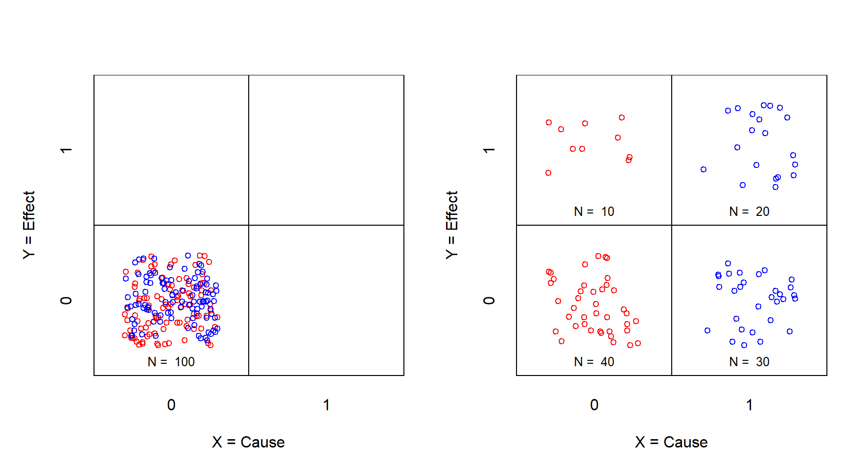
Figure 3.1: XY table of the traditional experiment before (left) and after (right) treatment. X = Treatment (0 = no; 1 = yes); Y = Effect (0 = no; 1 = yes). Red: control group; Blue: treatment group.
With a traditional RCT experiment, after the treatment usually all four cells have cases. In this example, 10 cases from the control group have moved from the lower-left cell to the upper-left cell, suggesting a time effect. The cases from the treatment group have all moved to \(X\) = 1. Treatment and the time had no effect on the 30 cases in the lower-right cell. Treatment and time did have an effect on the 20 cases in the upper-right cell. The data pattern in the four cells suggests that the treatment had an effect. There are more cases in the upper-right cell (resulting from a time effect and a treatment effect) compared to the number of cases in the upper left cell (resulting only from a time effect). The odds ratio is an estimate the “average treatment effect”: \((20/30)/(10/40) = 2.67\).
3.2.1.1 The sufficiency experiment
The sufficiency experiment can be considered as a special case of the traditional experiment, namely when after the manipulation (Figure 3.2), all cases of the treatment group are in the upper-right cell. Then the odds ratio for estimating the average effect is infinite, independently of the distribution of the cases in the control group: \((50/0)/(10/40) = \infty\). Note that this situation is named “perfect separation” and is considered a problem for “average effect” statistical analysis. In this situation \(X\) is called a “perfect predictor” that is normally left out from further analysis, because of the statistical problems. However, actually \(X\) is an very important predictor of the outcome: it ensures the outcome, hence the name “perfect predictor”.
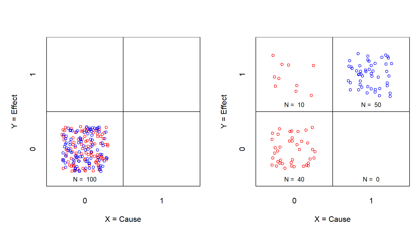
Figure 3.2: XY table of the sufficiency experiment before (left) and after (right) treatment. X = Treatment (0 = no; 1 = yes); Y = Effect (0 = no; 1 = yes). Red: control group; Blue: treatment group.
3.2.1.2 Non-necessity test
Referring to Figure 3.1, right, a part of the traditional “average treatment effect” experiment can be interpreted as a non-necessity test. While the emptiness in the lower-right cell reflects sufficiency, the emptiness of the upper-left cell reflects necessity. If this cell has cases due to the time effect, it can be concluded that the treatment is not necessary for the effect, because the effect is possible without the treatment. If this cell remains empty the necessity is not disconfirmed. This ‘non-necessity test’ as part of a traditional experiment can only be done with the control group. The treatment group cannot be used for testing necessity because it cannot test the emptiness of the upper-left cell. The non-necessity test with the control group is not an experiment since no manipulation is involved. It can be considered an observational study.
3.2.2 The necessity experiment
For testing the emptiness of the upper-left cell with an experiment (with manipulation of \(X\)), another approach is required. In the necessity experiment, all cases start to be in the upper-right cell (\(X\) = 1 and \(Y\) = 1) as illustrated in Figure 3.3, left.
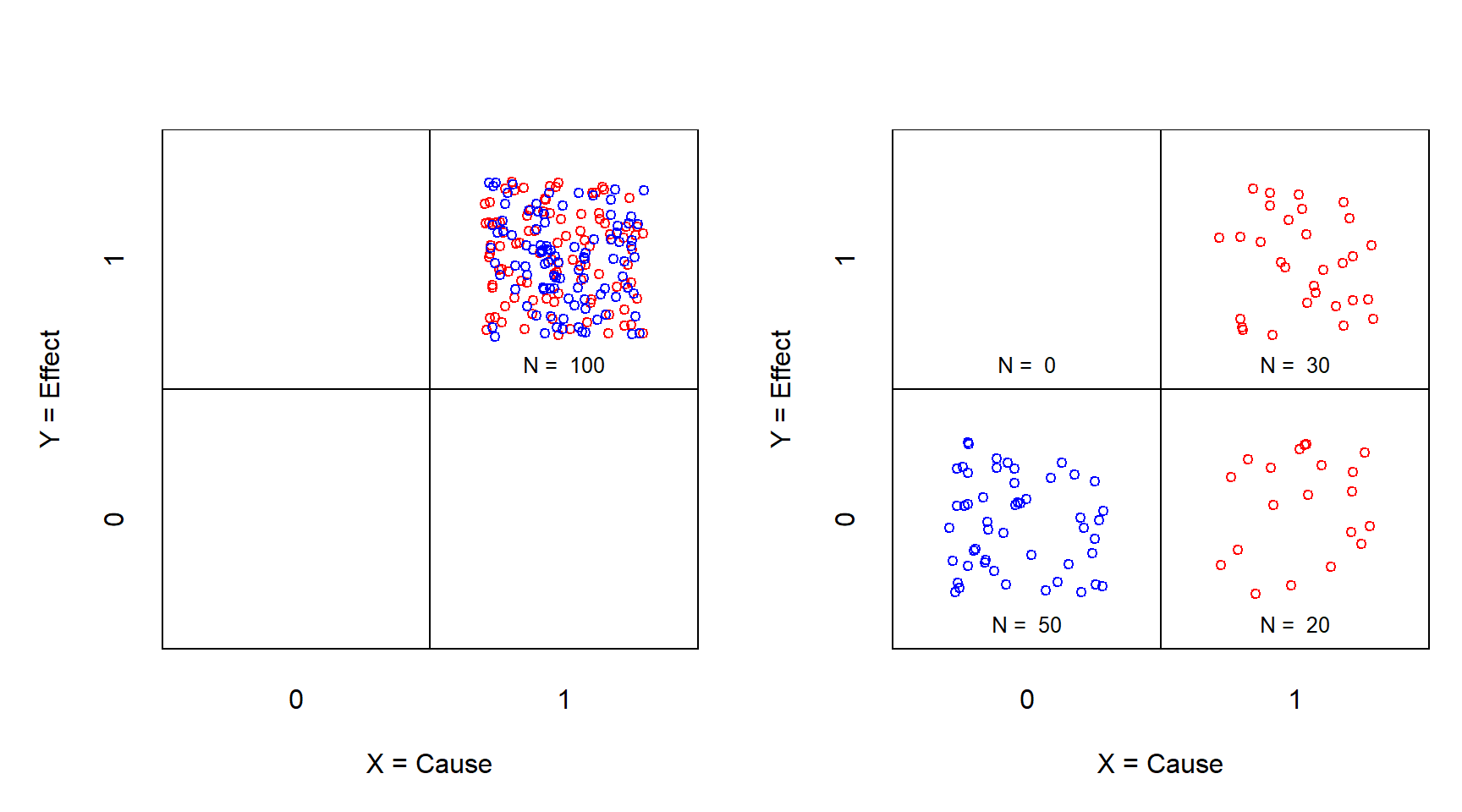
Figure 3.3: XY table of the necessity experiment before (left) and after (right) treatment. X = Treatment (0 = no; 1 = yes); Y = Effect (0 = no; 1 = yes). Red: control group; Blue: treatment group.
The manipulation consists of removing rather than adding the treatment (from \(X\) = 1 to \(X\) = 0) and it is observed whether this removes the outcome (from \(Y\) = 1 to \(Y\) = 0). This is illustrated in Figure 3.3, right. Necessity is supported when the upper-left cell remains empty. Like in a sufficiency experiment, the odds ratio is infinite. Also this situation is called “perfect separation” and is considered a problem for “average effect” statistical analysis, and \(X\) is called a “perfect predictor” that is normally left out from further analysis, because of the statistical problems. However, again \(X\) is an very important predictor of the outcome and indeed a “perfect predictor”: it ensures the absence of the outcome when \(X\) is absent. Again, the odds ratio for estimating the average effect is infinite, independently of the distribution of the cases in the control group: \((50/0)/(20/30) = \infty\).
3.2.2.1 The necessity experiment with continuous outcome and dichotomous condition
Figure 3.4 illustrates the situation when the outcome is a continuous variable. Before the manipulation the condition is present (\(X\) = 1). The \(Y\)-values of the cases include the maximum value of the outcome (\(Y\) = 1). Necessity is supported when after the manipulation the maximum value in the treatment group is reduced to a value of \(Y = Y_c\), resulting in an empty upper-left corner of the \(XY\) plot. The necessary condition can be formulated as \(X = 1\) is necessary for \(Y >= Y_c\). The necessity effect size is the empty area divided by the scope. In this example the effect size = 0.175.
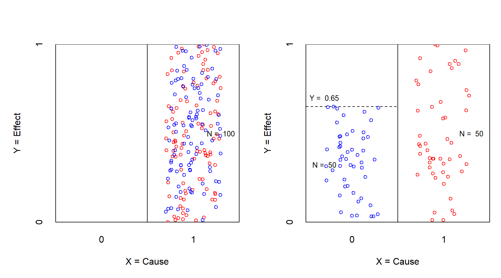
Figure 3.4: XY plot of the necessity experiment with continuous outcome before (left) and after (right) treatment. X = Treatment (0 = no; 1 = yes); Y = Effect between 0 and 1. Red: control group; Blue: treatment group.
3.2.2.2 The necessity experiment with continuous outcome and condition
In Figures 3.5, 3.6, 3.7, and 3.8 both the condition and the outcome are continuous variables. Rather than being a necessity experiment to test whether necessity exists, in this experiment an existing necessity is challenged. The manipulation consists of offering an experimental situation (e.g., an intervention or a scenario such as in a vignette study or a Monte Carlo experiment) that reduces the level of the condition in the treatment group but not in the control group. Necessity remains supported when after the manipulation no cases enter the empty zone. This is shown in Figure 3.5, where the necessity effect size before manipulation (0.25) stays intact after manipulation.
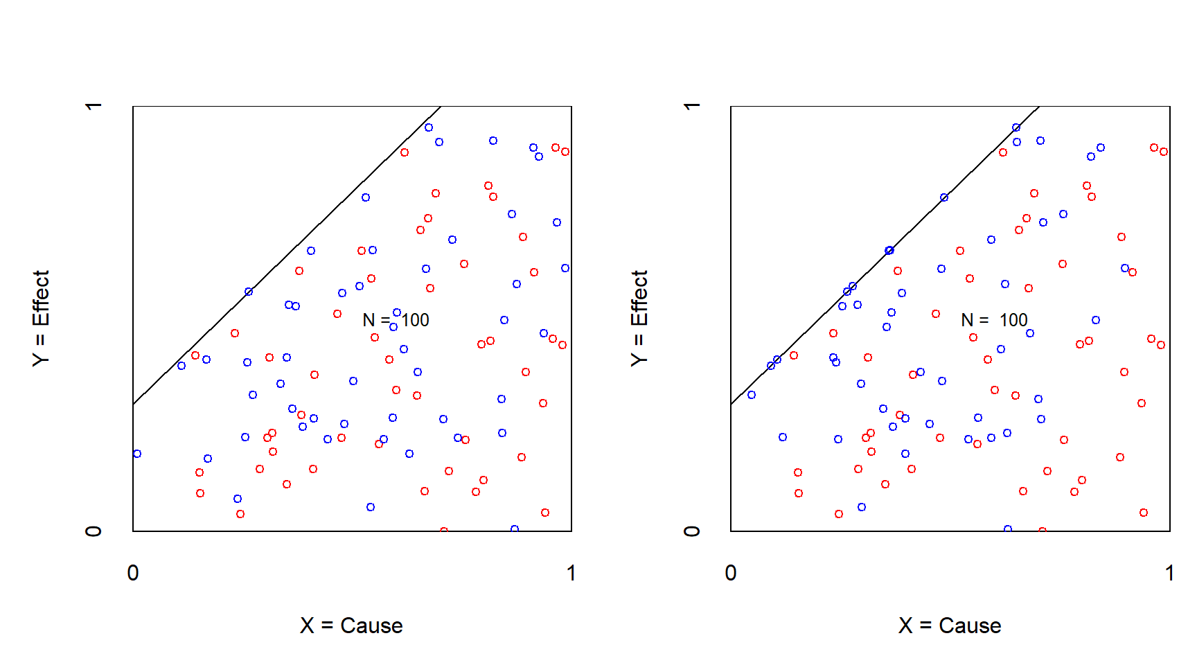
Figure 3.5: XY plot of an experiment to challenge necessit with continuous condition and outcome before (left) and after (right) treatment of reducing the X. Effect size remains after manipulation. Red: control group; Blue: treatment group.
However, when cases enter the empty zone, the necessity is reduced (smaller effect size) or rejected (no empty space). Figure 3.6 shows an example of a reduction of the necessaty effect size from 0.25 to 0.15.
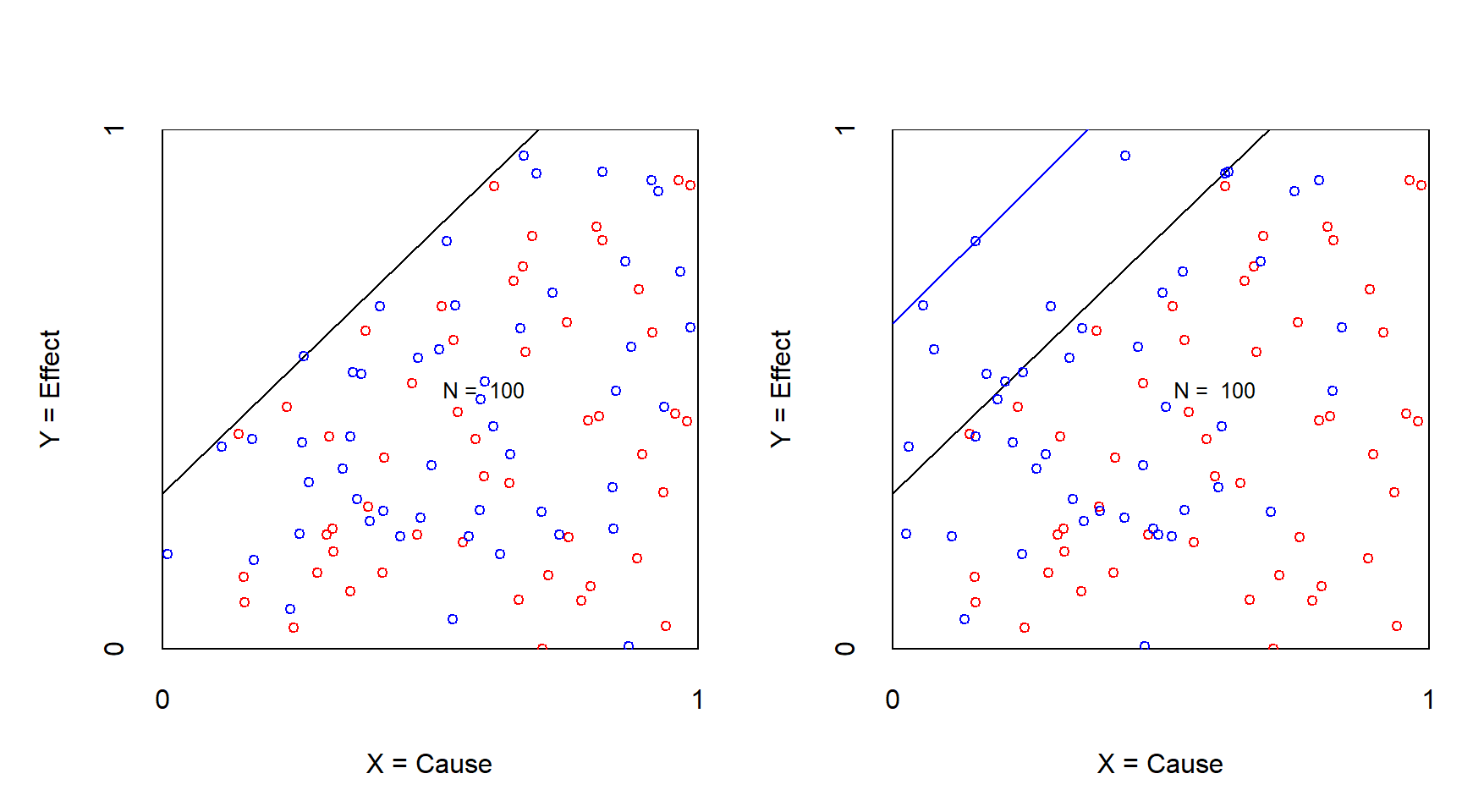
Figure 3.6: XY plot of an experiment to challenge necessity with continuous condition and outcome before (left) and after (right) treatment of reducing the X. Effect size reduces after manipulation. Red: control group; Blue: treatment group.
Figure 3.7 is an example of a rejection of a necessary condition after manipulation because the effect size disappears after manipulation.
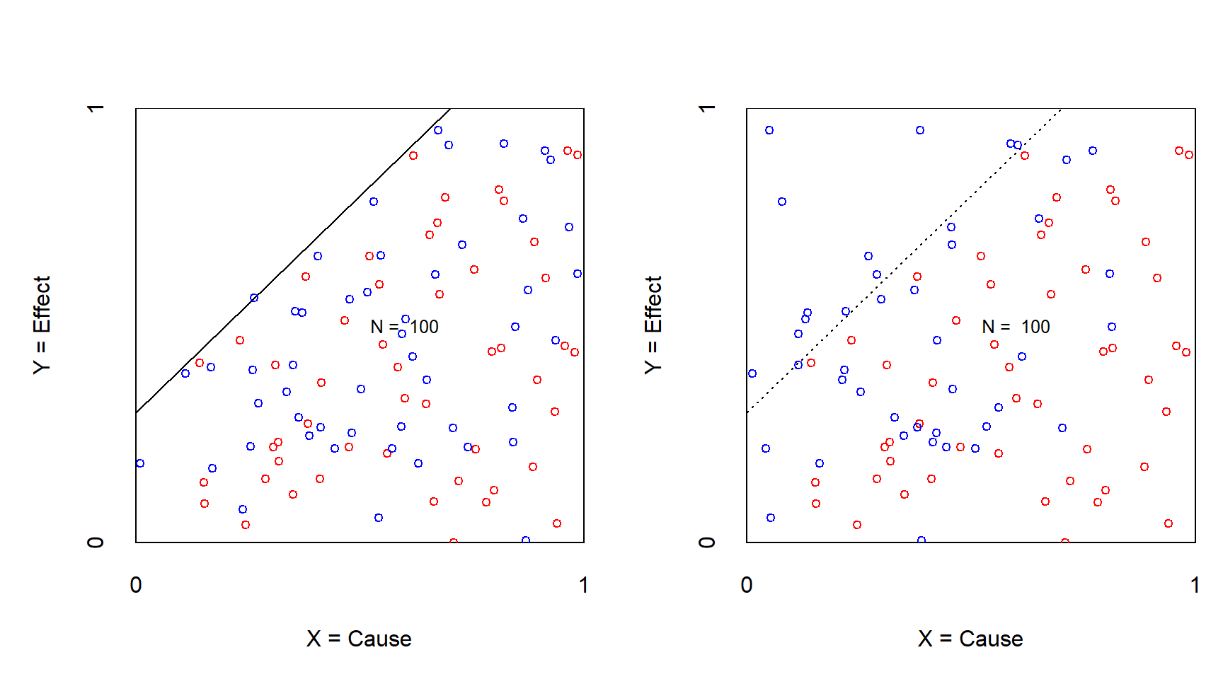
Figure 3.7: XY plot of an experiment to challenge necessity with continuous condition and outcome before (left) and after (right) treatment of reducing the X. Effect size disappears after manipulation. Red: control group; Blue: treatment group.
In rare situations before manipulation the necessary condition may be satisfied in all cases of the sample such that no empty space is present in the sample. After manipulation the hidden empty space becomes visible (see Figure 3.8).
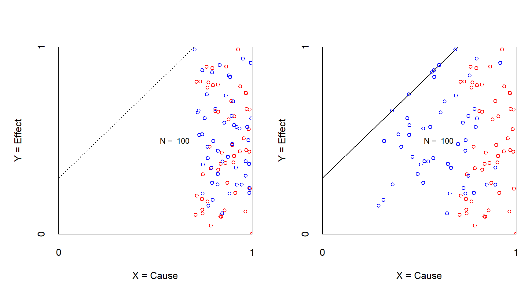
Figure 3.8: XY plot of an experiment to challenge necessity with continuous condition and outcome before (left) and after (right) treatment of reducing the X. Effect size appears after manipulation. Red: control group; Blue: treatment group.
3.3 Sample size
A frequently asked question is “What is the required sample size for NCA”. The short answer is: “The more the better, but at least N = 1”. This is explained below.
3.3.1 Small N studies
In hypothesis testing research a sample is used to test whether the hypothesis can be falsified (rejected) or not. After repeated non-rejections with different samples, a hypothesis may be considered ‘confirmed’.
When \(X\) and \(Y\) are dichotomous variables (e.g., having only two values ‘absent’ or ‘present’, ‘0’ or ‘1’, low or high) it is possible to falsify a necessary condition with even a single case (N = 1). The single case is selected by purposive sampling (not random sampling). The selected case must have the outcome (present, 1, high), and it is observed if this case has the condition or not. If not (absent, 0, low), the hypothesis is rejected. If yes (present, 1, high), the hypothesis is not rejected. In the deterministic view on necessity, where no exceptions exist, the researcher can conclude that the hypothesis is not rejected. For a stronger conclusion replications with other cases must be done.
An example of this approach is a study by Harding et al. (2002), who studied rampage school shootings in the USA. They first explored two shooting cases and identified five potential necessary conditions: gun availability, cultural script (a model why the shooting solves a problem), perceived marginal social position, personal trauma, and failure of social support system. Next, they tested these conditions with two other shooting cases, an concluded that their ‘pure necessity theory’ (see section 2.5) was not rejected.
In another example, Fujita & Kusano (2020) published an article in the Journal of East Asian Studies studying why some Japanese prime ministers (PM’s) have attempted to deny Japan’s violent past through highly controversial visits to the Yasukuni Shrine, while others have not. They propose three necessary conditions for a Japanese PM’s to decide to visit: a conservative ruling party, a government enjoying high popularity, and Japan’s perception of a Chinese threat. They tested these conditions by considering the 5 successful cases (PM’s who visited the shrine) from all 22 cabinets between 1986 and 2014. In these successful cases the three necessary conditions were present. This means that the hypotheses were not rejected. They additionally tested the contrapositive: the absence of at least one necessary condition is sufficient for the absence of a visit, which was also supported by the data.
The editor of the journal commented on the study as follows: https://www.youtube.com/watch?v=zHlVzsQg8Ek
Even in small N studies it is possible to estimate the p value when the number of cases is at least 4 (assuming that all \(X\)’s have different values, and all \(Y\)’s have different values). This can be explained as follows. The p value refers to the probability that the observed data pattern is obtained when the variables are unrelated. NCA’s statistical test compares the effect size of the observed sample (with N observed cases) with the effect sizes of created samples with N fictive cases when \(X\) and \(Y\) are unrelated. Fictive cases that represent non-relatedness between \(X\) and \(Y\) are obtained by combining observed \(X\) values with observed \(Y\) values into new samples. The total number of created samples with a unique combination (permutations) of fictive cases is N! (N factorial). Only one of the permutations corresponds to the observed sample. For each sample the effect size is calculated. The p value is then defined as the probability (p) that the effect size of the observed sample is equal to or larger than the effect size of all samples. If this probability is small (e.g., p < 0.05), a ‘significant’ result is obtained. This means that the observed sample is unlikely the result of a random process of unrelated variables (the null hypothesis is rejected), suggesting support for an alternative hypothesis. The p value helps to avoid a false positive conclusion, namely that the effect size is the result of a necessity relationship between X and Y, whereas actually it may be a random result of unrelated variables. For example, for a sample size of N = 2, the total number of unique samples or permutations (including the observed sample) is \(2! = 1*2 = 2\). When the observed sample consists of case 1 \((x_1,y_1)\) and case 2 \((x_2,y_2)\) then the observed x-values \((x_1,x_2)\) and the observed y-values \((y_1,y_2)\) can be combined into two unique samples of size N = 2: the observed sample with observed case 1 \((x_1, y_1)\) and observed case 2 \((x_2, y_2)\), and the alternative created sample of N = 2 with two fictive cases \((x_1, y_2)\) and \((x_2, y_1)\). For example, when the observed sample has case 1 is \((0,0)\) and case 2 is \((1,1)\) the observed effect size with empirical scope is 1. The effect size of the alternative sample has the cases \((1,0)\) and \((0,1)\) with effect size 0. The probability that the effect size of the observed sample is equal to or larger than the effect sizes of the two samples is 1 in 2, thus p = 0.5. This means that the observed effect size of 1 is a ‘non-significant’ result because the probability that the observed effect size is caused by unrelated variables is not small enough (not below 0.05).
Similarly, for sample size N = 3 the total number of unique samples is \(3! = 1*2*3 = 6\), and the smallest possible p value is \(1/6 = 0.167\), for N = 4 the total number of unique samples is \(4! = 1*2*3*4 = 24\), and the smallest possible p value is \(1/24 = 0.042\), and for N = 5 the total number of unique samples is \(5! = 1*2*3*4*5 = 120\), and the smallest possible p value is \(1/120 = 0.008\), etc. Thus, only from N = 4 it is possible to obtain a p value that is small enough for making conclusions about the ‘statistical significance’ of an effect size.
When sample size increases, the total number of unique samples increases rapidly, and the possible p value decreases rapidly. For N = 10 the total number of samples (permutations) is 3628800 and the corresponding possible p value is smaller than 0.0000003. For N = 20 is the total number of samples is a number of 19 digits with a corresponding possible p value that has 18 zero’s after the decimal point. When N is large the computation of the effect sizes of all samples (permutations) requires unrealistic computer times. Therefore, NCA’s uses a random sample from all possible samples (permutations) and estimates the p value with this selection of samples. Therefore, NCA’s statistical test is an ‘approximate permutation test’. In the NCA software this test is implemented with the test.rep argument in the nca_analysis function to provide the number of samples to be analyzed, for example 10000 (the larger the more precision but also more computation time). When the test.rep value is larger than N! (which can happen for small N), the software selects all N! samples for the p value calculation.
3.3.2 Large N studies
In large N studies cases are sampled from a population in the theoretical domain. The goal of inferential statistics is to make an inference (statistical generalization) from the sample to the population. The ideal sample is a probability sample where all cases of the population have equal chances to become part of the sample. This contrasts convenience sample where cases are selected from the population for convenience of the researcher, for example because the researcher has easy access to the case. NCA puts no new requirements on sampling, and common techniques that are used with other data analysis methods can also be applied for NCA, with the same possibilities and limitations.
3.4 Quantitative data
Quantitative data are data expressed by numbers where the numbers are scores (or values) with a meaningful order and meaningful distance. Scores can have two levels (dichotomous, e.g. 0 and 1 ), a finite number of levels (discrete, e.g. 1,2,3,4,5) or an infinite number of levels (continuous, e.g. 1.8, 9.546, 306.22).
NCA can be used with any type of quantitative data. It is possible that a single indicator represents the concept (condition or outcome) of interest. Then this indicator score is used to score the concept. For example, in a questionnaire study where a subject or informant is asked to score conditions and outcomes with seven-point Likert scales, the scores are one of seven possible (discrete) scores.
It is also possible that a construct that is build from several indicators is used to represent the concept of interest. Separate indicator scores are then summed, averaged or otherwise combined (aggregated) by the researcher to score the concept. It is also possible to combine several indicator scores statistically, for example by using the factor scores resulting from factor analysis, or construct score of latent variables resulting from the measurement model of a Structural Equation Model.
Quantitative data can be analysed with NCA’s ‘scatter plot approach’ and with NCA’s software for R. When the number of variable levels is small (e.g. less than 5) it is also possible to use NCA’s contingency table approach.
3.5 Qualitative data
Qualitative data are data expressed by names, letters or numbers without a quantitative meaning. For example, gender can be expressed with names (‘male’, ‘female’, ‘other’), letters (‘m’, ‘f’, ‘o’) or numbers (‘1’, ‘2’, ‘3’). Qualitative data are discrete and have usually no order between the scores (e.g., names of people) or if there is an order, the distances between the scores are unspecified (e.g. ’low, medium, high). Although with qualitative data a quantitative NCA, (with the NCA software for R) in not possible, it is still possible to apply NCA in a qualitative way using visual inspection of the \(XY\) contingency table or scatter plot.
When the condition is qualitative the researcher observes for a given score of \(Y\), which qualitative score of the condition (e.g., ‘m’, ‘f’, ‘o’) can reach that score of \(Y\). When the logical order of the condition is absent, the position of the empty space can be in any upper corner (left corner, middle or right; assuming the hypotheses that \(X\) is necessary for the presence of or a high level of \(Y\)). When a logical order of the qualitative scores is present, the empty space is in the upper left corner (assuming the hypotheses that the presence of a high level of \(X\) is necessary for the presence of or a high level of \(Y\)). In both cases the size of the empty space is arbitrary and the effect size cannot be calculated because the values of \(X\) and therefore the effect size are meaningless. However, when \(Y\) is quantitative, the distance between the highest observed \(Y\) score and the next-highest observed \(Y\) score could be an indication of the constraint of \(X\) on \(Y\).
3.6 Longitudinal, panel and time-series data
Researchers often use cross-sectional research designs. In such designs several variables are measured at one moment in time. In a longitudinal research design the variables are measured at several moments in time. The resulting data are called longitudinal data, panel data or time-series data. In this book, longitudinal data (a name commonly used by statisticians) and panel data (a name commonly used by econometricians) are considered as synonyms.
Longitudinal/panel data are data from a longitudinal/panel study in which several variables are measured at several moments in time. Time-series data are a special case of longitudinal/panel data in which one variable is measured many times.
Longitudinal/panel and time-series data can be analysed with NCA with different goals in mind. Two straightforward ways are discussed in this book. First, if the researcher is not specifically interested in time, the time data can be pooled together as if the data were from cross-sectional data set (e.g., Jaiswal & Zane, 2022b). Second, if the researcher is interested in time trends, NCA can be applied for each time stamp separately.
3.6.1 NCA with pooled data
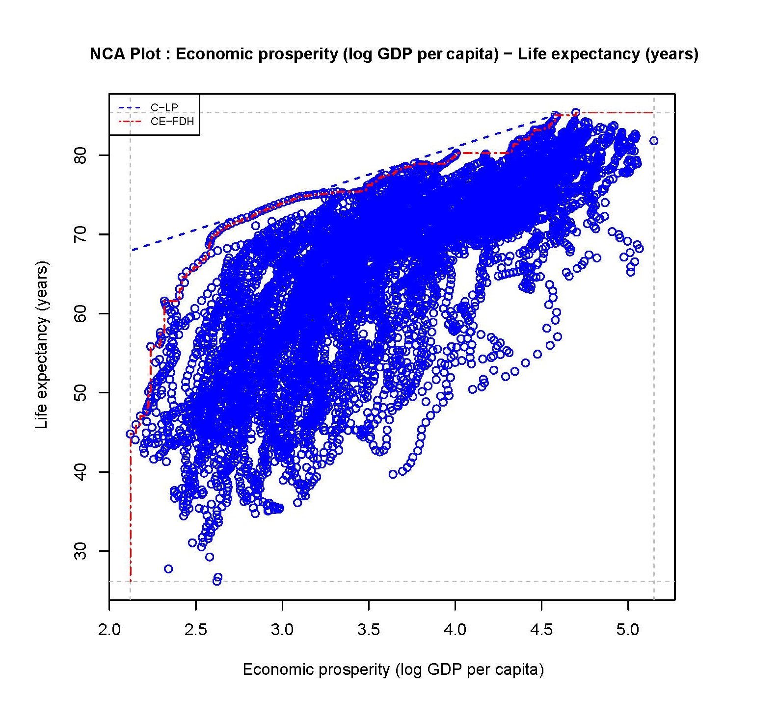
Figure 3.9: Scatter plot of Economic prosperity and Life expectancey with two ceiling lines (Pooled Worldbank data from 1960 to 2019 for all countries/years).
Figure 3.9 shows an example of a scatter plot of a time-pooled data. It is an example of the necessity of a country’s economic prosperity for a country’s average life expectancy: A high expected age is not possible without economic prosperity. This necessity claim can be theoretically justified by the effect of economic prosperity on the quality of the health care system. The data are from the Worldbank for 60 years between 1960 and 2019 and for 199 countries. Data is available for 8899 country-years. The scatter plot of time pooled data has Economic prosperity expressed as log GDP per capita on the \(X\) axis, and Life expectancy at birth expressed in years on the \(Y\) axis.
Figure 3.9 shows a clear empty space in the upper left corner. The NCA analysis is done with the C-LP ceiling line, which is a straight ceiling line that has no observations above it, and with the
CE-FDH line that follows the somewhat non-linear trend of the upper left border
between the full and empty space. The empty space in the upper left corner indicates that a certain level of life expectancy is not possible without a certain level of economic prosperity. For example, for a country’s life expectancy of 75 years, a economic prosperity of at least 3 (103 = 1000 equivalent US dollar) is necessary. The effect sizes for the two ceiling techniques are 0.13 (p < 0.001) and 0.16 (p < 0.001), respectively. This suggests that a necessity
relationship exists between Economic prosperity and Life expectancy.
(There is also a well-known positive average relationship (imaginary line through the middle of the data), but this average trend is
not considered here. Furthermore, the lower right corner is empty as well suggesting that the absence of \(X\) is necessary for the absence of \(Y\), which could be evaluated with the corner = 4 argument in the nca_analysis function of the NCA software.)
3.6.2 NCA for describing time trends
When the researcher is interested in time trends, NCA can be applied for each time stamp separately. Such approach can be considered a multiple cross-sectional NCA analysis. As an example in Table 3.1 a longitudinal analysis is done with the same countries and years as in Figure 3.9, but now analysed per year and using only the C-LP ceiling line. For making the NCA results comparable per year, the scope for each year is standardized to the scope of the pooled data (based on the absolute minima and maxima of empirically observed Economic prosperity and Life expectancy in the data). This scope is entered in the NCA analysis as the theoretical scope for each year.
Table 3.1 shows several NCA parameters for each time-point. The effect sizes range from 0.13 to 0.29 and the p values for all years is less than 0.001. In general, the effect size decreases over the years, such that the constraint that economic prosperity puts on life expectancy is decreasing over time.

Figure 3.10: Animation with countries per year with the ceiling line in red.
Figure 3.10 is an animated figure showing the time trends. In the figure, each data point is a country. The size of a data point refers to the country’s population size, and the color to the geographic region to which it belongs, e.g., yellow for the Sub-Saharan region, and violet for East Asian and Pacific region.
3.6.3 Interpretation
The interpretation of longitudinal analysis with NCA focuses on the change of the effect size and ceiling line over time. For example, Table 3.1 shows that the size of the necessity effect of economic prosperity for life expectancy reduces over time. This indicates that economic prosperity has become less of a bottleneck for high life expectancy. Figure 3.10 shows that this decrease of effect size is particularly due to the increase of the intercept (upward moving of the ceiling line). This indicates a rise of the maximum possible life expectancy for a given level of prosperity.
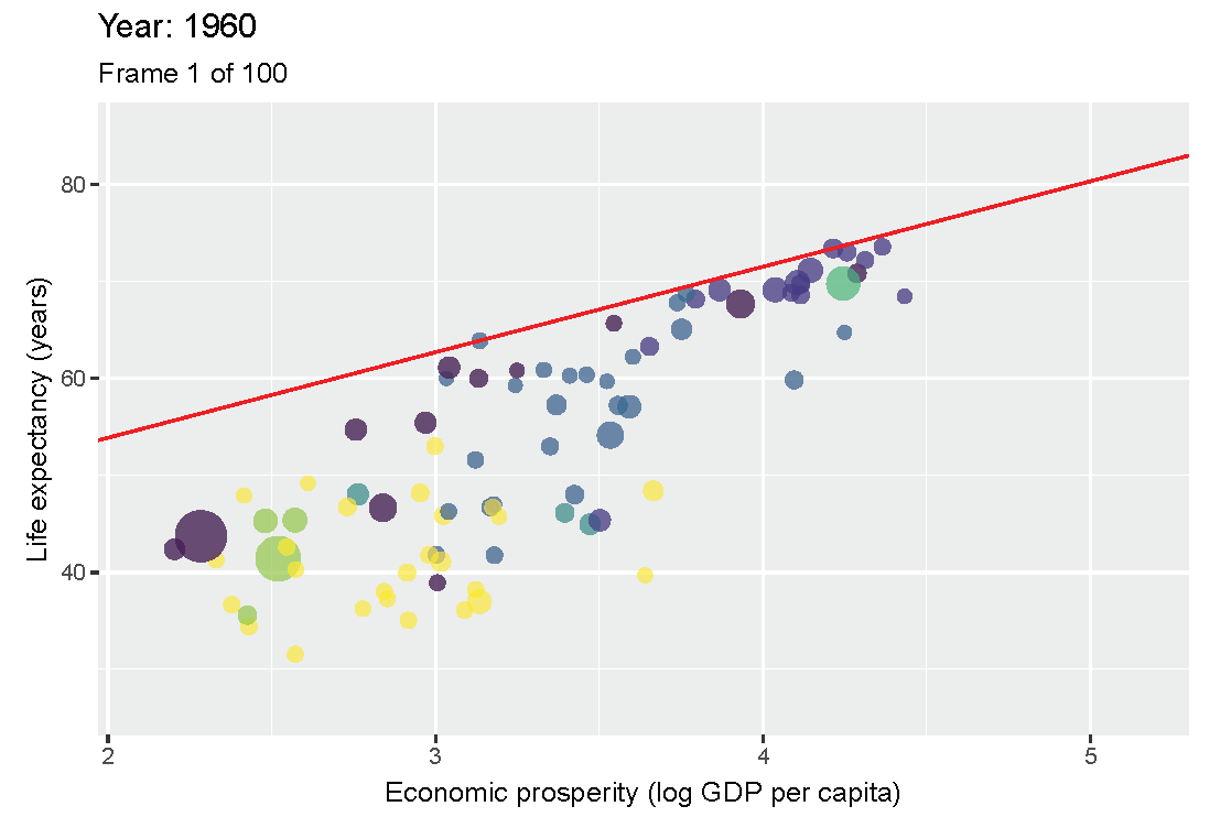
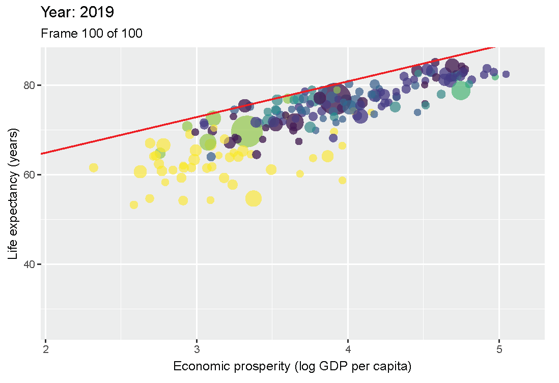
Figure 3.11: Scatter plot of Economic prosperity and Life expectancey for 1960 and 2019.
Figure 3.11 shows that in 1960 the maximum life expectancy for a prosperity of 3.4 (103.4 = 2500 equivalent US dollars) was about 65 years, and in 2019 it was about 75 years. The reduction of necessity is also partly due to the flattening of the ceiling line, indicating that the difference between the best performing less prosperous countries, and the best performing more prosperous countries, is diminishing. In 1960 countries with prosperity of 3.4 (2500 dollar) had a maximum possible life expectancy that was 10 years less than that for countries with prosperity of 4.4 (25000 dollar): 65 versus 75 years. However, in 2019 countries with prosperity of 3.4 (2500 dollar) had a maximum possible life expectancy that was only 5 years less than that for countries with prosperity of 4.4 (25000 dollar): 75 versus 80 years.
Another observation is that the density of countries near the ceiling line has increased over the years. This indicates that the relative differences in life expectancy between the more and less performing countries has reduced.
Socio-economic policy practitioners could probably make new interesting interpretations from these necessity trends. For example, in the past, economic prosperity was a major bottleneck for high life expectancy. Currently, most countries (but surely not all) are rich enough for having a decent life expectancy of 75 years; if these countries do not reach that level of life expectancy, other factors than economic prosperity are the reason that it is not achieved. In the future, economic prosperity may not be a limiting factor for high life expectancy when all countries have reached an GDP per capita of 2500 dollar and the empty space in the upper left corner has disappeared.
3.7 Set membership data
NCA can be used with set membership scores. This is usually done when NCA is combined with QCA. In QCA ‘raw’ variable scores are ‘calibrated’ into set membership scores with values between 0 and 1. A set membership score indicates to which extend a case belongs to the set of cases that have a given characteristic, in particular the \(X\) and the \(Y\). Several studies have been published that use NCA with set membership data (e.g., Torres & Godinho, 2022). These studies combine NCA with QCA for gaining additional insights (in degree) about the conditions that must be present in all sufficient configurations. Section 4.7 discusses how NCA can be combined with QCA.
3.8 Outliers
Outliers are observations that are “far away” from other observations. Outliers can have a large influence on the results of any data analysis, including NCA. In NCA an outlier is an ‘influential’ case or observation that has a large influence on the necessity effect size when removed.
3.8.1 Outlier types
Because the effect size is defined by the numerator ceiling zone divided by the denominator scope and an outlier is defined by its influence on the effect size, two types of outliers exist in NCA: an ‘ceiling zone outlier’ and a ‘scope outlier’.
A ceiling zone outlier is an isolated case in the otherwise empty corner of the scatter plot that reflects necessity (usually the upper left corner). Such case determines the location of the ceiling line, thus the size of the ceiling zone, and thus the necessity effect size. When a ceiling zone outlier is removed, it usually increases the ceiling zone and thus increases the necessity effect size.
A scope outlier is an isolated case that determines the minimum or maximum value of the condition or the outcome, thus the scope, and thus the necessity effect size. When a scope outlier is removed, it usually decreases the scope and thus increases the effect size.
When a case is both a ceiling zone outlier and a scope outlier, it determines the position of the ceiling and the minimum or maximum of value of \(X\) or \(Y\). When such case is removed it simultaneously decreases the ceiling zone and the scope. The net effect is often is a decrease of the necessity effect size.
When duplicate cases determine the ceiling line or the scope the effect size will not change when only one of the duplicate cases is removed. Single cases that have a duplicate have no influence on the effect size when removed, and therefore are no candidates for potential outliers, unless a duplicate set cases is defined as outlier and removed. Cases that are below the ceiling line and away from the extreme values of \(X\) and \(Y\) are not potential outliers.
It depends on the ceiling line technique which cases are candidates for potential ceiling zone outliers. The CE-FDH and CR-FDH ceiling techniques use the upper left corner points of the CE-FDH ceiling line (step function) for drawing the ceiling line. These upper left corner points are called ‘peers’. Therefore, the peers are potential outliers when these ceiling lines, which are the default lines of NCA, are used. The C-LP ceiling line uses only two points of the peers for drawing the ceiling line, and these points can therefore be potential ceiling zone outliers. The scope outliers do not depend on the ceiling technique.
3.8.2 Outlier identification
There are no scientific rules for deciding if a case is an outlier. This decision depends primarily on the judgment of the researcher. For a first impression of possible outliers, the researcher can visually inspect the scatter plot for cases that are far away from other cases. In the literature rules of thumb are used for identifying outliers. For example, a score of a variable is an outlier score ‘if it deviates more than three standard deviations from the mean’, or ‘if 1.5 interquartile ranges is above the third quartile or below the first quartile’. These pragmatic rules address only one variable (\(X\) or \(Y\)) at a time. Such single variable rules of thumb may be used for identifying potential scope outliers (unusual minimum and maximum values of condition or outcome). These rules are not suitable for identifying potential ceiling zone outliers. The reason is that ceiling zone outliers depend on the combination of \(X\) and \(Y\) values. For example, a case with a non-extreme \(Y\)-value may be a regular case when it has a large \(X\) value, because it does not define the ceiling. Then removing the case does not change the effect size. However, when \(X\) is small the case defines the ceiling and removing the case may change the effect size considerably. This means that both \(X\) and \(Y\) must be considered when identifying ceiling zone outliers in NCA.
No pragmatic bivariate outlier rules currently exist for NCA. Because a case is a potential outlier if it considerably changes the necessity effect size when it is removed, the researcher can first select potential outlier and then calculate the effect size change when the case is removed. If no clear potential outlier case can be identified, the researcher may decide that the data set does not contain outliers.
All potential ceiling zone outliers and potential scope outliers can be evaluated one by one by calculating the absolute and relative effect size changes when the case is removed (with replacement). An outlier may be identified if the change is ‘large’ –according to the judgment of the researcher–. Again, no scientific rules exist for what can be considered as a ‘large’ effect size change. In my experience single cases that change the effect size more than 30% when removed could be serious outliers, worth for a detailed further assessment. This does not mean that these cases are outliers, nor that single cases that change the effect size less than 30% are not outliers.
The NCA software from version 3.2.0 includes the nca_outliers function to evaluate potential outliers in a scatter plot. For illustration an outlier analysis is done with the example that is part of the NCA software to test the hypothesis that a country’s Individualism is necessary for a country’s Innovation performance. Data are available for 28 cases (countries).
library(NCA)
data(nca.example)
model <- nca_analysis(nca.example, 1,3)
nca_output(model, plots=TRUE, summaries =FALSE)
The scatter plot with the two default ceiling lines is shown in Figure 3.12.
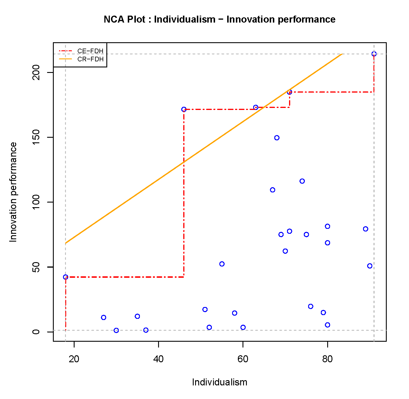
Figure 3.12: Scatter plot of nca.example
From visual inspection no clear outlier case that is very far away from the other case can be recognized.
The nca_outliers function can evaluate potential outliers in a scatter plot as follows:
##      outliers eff.or eff.nw dif.abs dif.rel ceiling scope
## 1 Japan         0.42   0.55    0.14    32.7       X
## 2 USA           0.42   0.33   -0.09   -21.5       X     X
## 3 Sweden        0.42   0.43    0.02     3.6       X
## 4 South Korea   0.42   0.40   -0.01    -3.0       X     X
## 5 Finland       0.42   0.42    0.00     0.2       X
## 6 Mexico        0.42   0.42    0.00     0.1             X
The output table shows in the first column the case names of the potential outliers. The second column displays the original effect size when no cases are removed (eff.or) and the third column displays the new effect size when the outlier is removed (eff.nw). The fourth column shows the absolute difference (dif.abs) between the new and the original effect sizes, and the fifth column the relative difference (dif.rel) between the new and the original effect sizes expressed as a percentage. A negative sign means that the new effect size is smaller than the orginal effect size.
The output shows six potential outliers. The new effect sizes range from 0.33 to 0.55, absolute differences range from -0.09 to +0.14, and relative differences range from -21.5% to +32.7%. Five outliers are ceiling zone outliers and three are scope outliers. It is possible that a case can be both types of outlier. South Korea defines the ceiling line and is thus a potential ceiling zone outlier, and it also defines the minimum \(X\) and is a potential scope outlier. USA is also both a ceiling zone outlier and a scope outlier because it defines the ceiling line and the maximum \(X\) and the maximum \(Y\). Mexico does not define the ceiling line but defines the minimum \(Y\). Finland, Japan and Sweden define the ceiling line but not the minimum or maximum value of \(X\) or \(Y\).
For visual inspection of the outliers in the scatter plot, the plotly = TRUE argument in the nca_outliers function displays an interactive scatter plot with highlighted outliers (plot not shown here):
As expected, the three potential outliers that are only ceiling zone outliers (Finland, Japan, Sweden) increase the effect size when removed. Their absolute differences range from virtually 0 to 0.14, and their relative effect size differences from 0.2% to 32.7%. As expected, the potential outlier that is only an potential scope outlier (Mexico) increases the effect size when removed, but this influence is marginal. As expected, the two potential ceiling zone outliers that are also potential scope outliers reduce the effect size when removed (South Korea and USA) with absolute effect size differences of -0.01 and -.0.09, respectively, and relative effect size differences of -3.0% and - 21.5%, respectively. All other cases are no potential outliers because they have no influence on the effect size when removed.
The two default ceiling lines CE-FDH and CR-FDH have the same potential outliers. For other ceiling lines the outliers can be different. For example, the C-LP ceiling technique selects two cases for drawing the ceiling line, and therefore only these two cases can be potential ceiling zone outliers. The ceiling line can be specified with the ceiling argument in the nca_outliers function as follows:
##      outliers eff.or eff.nw dif.abs dif.rel ceiling scope
## 1 USA           0.16   0.06   -0.11   -65.3       X     X
## 2 South Korea   0.16   0.14   -0.02   -12.3       X     X
## 3 Mexico        0.16   0.16    0.00     0.1       X     X
Note that after a potential outlier is removed and the effect size difference is calculated, the case is added again to the data set before another potential outlier is evaluated (removing with replacement).
With the nca_outlier function it is also possible to evaluate two or more potential outliers at once by specifying k (= number of outliers). This evaluates the change of effect size when k potential outliers are removed at once. For example, a researcher can evaluate two potential outliers as follows:
##               outliers eff.or eff.nw dif.abs dif.rel ceiling scope
## 1  Japan - Finland       0.42   0.59    0.18    42.3       X
## 2  Japan - South Korea   0.42   0.58    0.16    38.8       X     X
## 3  Japan - Sweden        0.42   0.57    0.15    36.4       X
## 4  Japan - Austria       0.42   0.56    0.14    34.0       X
## 5  Japan - Mexico        0.42   0.55    0.14    32.9       X     X
## 6  Japan                 0.42   0.55    0.14    32.7       X
## 7  Japan - Portugal      0.42   0.55    0.14    32.7       X
## 8  Japan - Greece        0.42   0.55    0.14    32.7       X
## 9  Japan - Spain         0.42   0.55    0.14    32.7       X
## 10 Japan - Germany       0.42   0.55    0.14    32.7       X
## 11 Japan - Switzerland   0.42   0.55    0.14    32.7       X
## 12 Japan - Australia     0.42   0.55    0.14    32.7       X
## 13 Japan - Turkey        0.42   0.55    0.14    32.7       X
## 14 USA - Sweden          0.42   0.30   -0.12   -28.3       X     X
## 15 USA - South Korea     0.42   0.31   -0.10   -24.9       X     X
## 16 USA                   0.42   0.33   -0.09   -21.5       X     X
## 17 USA - Portugal        0.42   0.33   -0.09   -21.5       X     X
## 18 USA - Greece          0.42   0.33   -0.09   -21.5       X     X
## 19 USA - Spain           0.42   0.33   -0.09   -21.5       X     X
## 20 USA - Austria         0.42   0.33   -0.09   -21.5       X     X
## 21 USA - Germany         0.42   0.33   -0.09   -21.5       X     X
## 22 USA - Switzerland     0.42   0.33   -0.09   -21.5       X     X
## 23 USA - Turkey          0.42   0.33   -0.09   -21.5       X     X
## 24 USA - Mexico          0.42   0.33   -0.09   -21.4       X     X
## 25 USA - Finland         0.42   0.33   -0.09   -21.3       X     X
## # Not showing 44 possible outliersThe output shows the combinations of two potential outliers with the largest influence on the effect size when the combination is removed. The output also include single potential outliers when the single potential outlier has a similar influence on the effect size as combinations of potential outliers. A combination of more than 2 outliers is also possible; for larger data sets this may increase the computation time may considerably.
A potential outlier combination consists always of a single ceiling outliers or a single scope outlier (or both) as indicated in the output. When more k > 1 the plotly scatter plot only shows the single outliers in red as for k = 1.
From the example it appears that Japan is the most serious potential outlier.
3.8.3 Outlier decision approach
After a potential outlier is identified, the next question is what to do with it. NCA employs a two step approach for making a decision about an outlier. In the first step it is evaluated whether the outlier is caused by a sampling or measurement error. In the second step it is decided if an ‘outlier for unknown reasons’ should be part of the phenomenon (using the deterministic perspective on necessity) or should be considered an exception (using the typicality perspective on necessity, see Dul, 2024a).
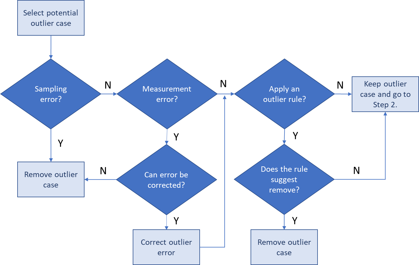
Figure 3.13: Outlier decision tree for Step 1 of the outlier decision approach.
The decision tree for the first step of NCA’s outlier decision approach is illustrated in Figure 3.13. First, the potential outlier case is selected. Next it is evaluated for sampling error. Sampling error refers a case that is not part of the theoretical domain of the necessity theory that is hypothesized by the researcher. For example, the case may be a large company, whereas the necessity theory applies to small companies only. A outlier case that is a sampling error should be removed from further analysis. If there is no sampling error, the potential outlier case may have measurement error. The condition or the outcome may have been incorrectly scored, which could happen for a variety of reasons. If there is measurement error but the error can be corrected, the outlier case becomes a regular case is kept for the analyses. If the measurement error cannot be corrected two situations may apply. If the measurement error is in the score of the outcome, the case should be removed from further analysis of all necessary conditions (if there are multiple necessary conditions). If the measurement error is in the score of the condition value, the case should be removed from further analysis of that condition, but the researcher may want to keep the case for the analysis of other conditions (as the case may not be an outlier for other conditions). If the the outlier is not caused by sampling error or measurement error or if no information about sampling error or measurement error is available, the outlier may be considered an ‘outlier for unknown reasons’. The researcher may then decide to apply an outlier rule that decides whether the case is kept or removed. Existing mono-variate outlier rules may be used for scope outliers in NCA. For example, a case may be considered an outlier if it is three standard deviations away from the mean of the condition or the outcome. For bi-variate ceiling outliers no generally accepted outlier rule exists. Such outlier rule may be stated by the researcher, for example based on the magnitude of the absolute or relative effect size changes when the case is removed (see section 3.8.2). Outlier rules should be specified and justified. If no outlier rule is applied the potential outlier case is kept and the next step of NCA’s outlier decision approach begins.
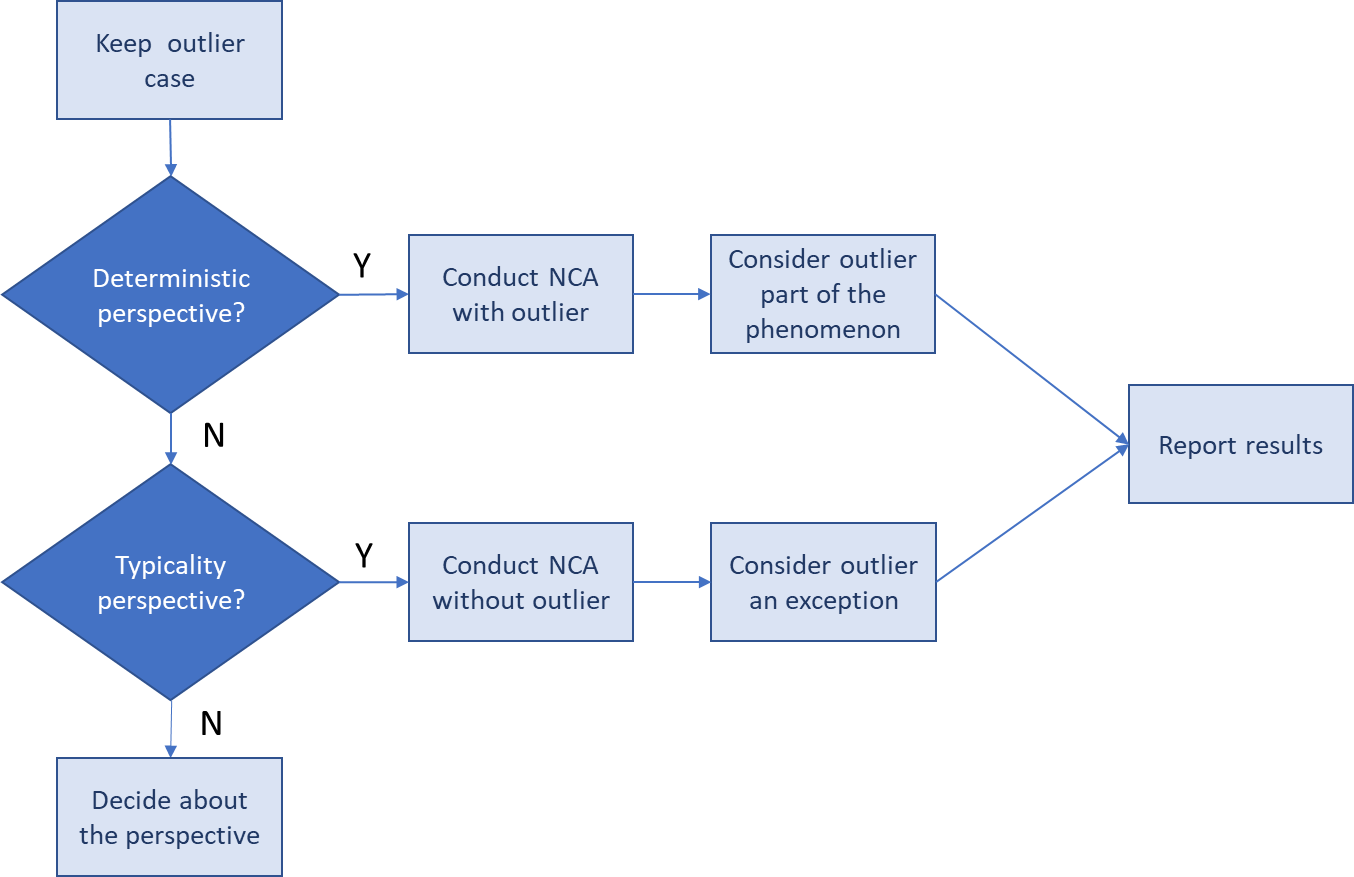
Figure 3.14: Outlier decision tree for for Step 2 of the outlier decision approach.
The decision tree for the second step is illustrated in Figure 3.14. The second step starts with the researcher’s decision about the causal necessity perspective. Two perspectives are distinguished for necessity causality (Dul, 2024a). The deterministic perspective can be formulated as ‘if \(X\) then always \(Y\)’. This perspective does not allow exceptions. An outlier for unknown reasons is then considered to be part of the phenomenon of interest, and the analysis is done with the outliers. The typicality perspective can be formulated as ‘if \(X\) then typically \(Y\)’. This perspective does allows exceptions. An outlier for unknown reasons is then considered to be an exception. The analysis is done without the outlier. When reporting the results, the exceptions are discussed as well.
It is the choice of the researcher to adopt a deterministic or typicality perspective on NCA. Handling an outlier is a decision made by the researcher. If another outlier decision is plausible as well, it is advised to perform a robustness check to evaluate the sensitivity of the results (see section 4.4).