Chapter 4 Data analysis
4.1 Visual inspection of the scatter plot
The starting point for NCA’s data analysis is a visual inspection of the \(XY\) scatter plot. This is a qualitative examination of the data pattern. By visual inspection the following questions can be answered:
- Is the expected corner of the \(XY\) plot empty?
- What is an appropriate ceiling line?
- What are potential outliers?
- What is the data pattern in the rest of plot?
Visual inspection of the scatter plot is illustrated with nca.example, in particular for testing of the hypothesis that Individualism is necessary for Innovation performance. Figure 4.1 shows the scatter plot of Individualism versus Innovation performance with all 28 cases as black dots.
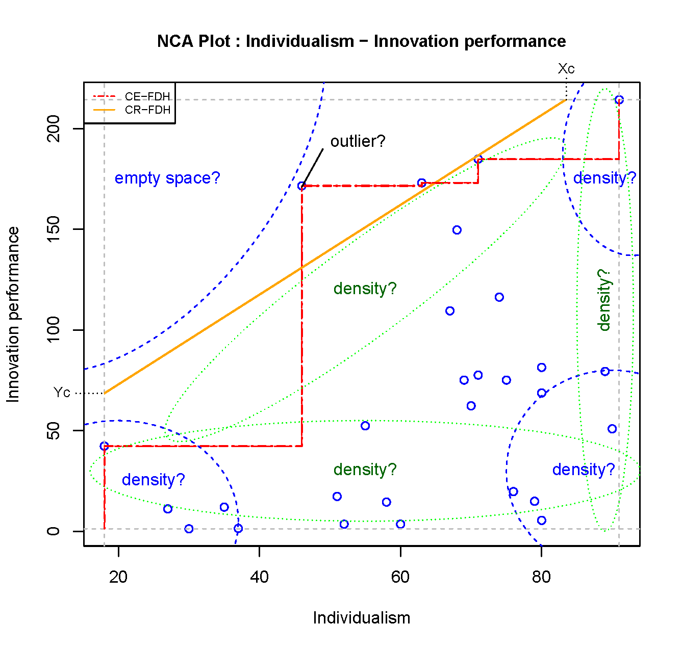
Figure 4.1: Scatter plot of Individualism and Innovation performance for evaluating the empty space, the appropriateness of the ceiling line, potential outliers, and the density of the cases in relevant areas.
4.1.1 Is the expected corner empty?
According to the hypothesis a high level of \(X\) is necessary for a high level of \(Y\) such that the upper left corner is expected to be empty. Figure 4.1 shows that cases with a low value of \(X\) have a low value of \(Y\), and that cases with a high value of \(Y\) have a high value of \(X\). The upper left corner is indeed empty. NCA’s effect size quantifies the size of the empty area in the scatter plot. After visual inspection the size of the empty space can be obtained with the NCA software by using the summaries argument of the nca_output function.
4.1.2 What is an appropriate ceiling line?
The ceiling line represents the border between the area with cases and the area without cases. Figure 4.1 shows the two default ceiling lines. The CR-FDH ceiling is often selected when the border is theoretically assumed to be linear, or when the condition and outcome have many levels (e.g., are continuous). The CE-FDH ceiling is often selected when the condition or outcome have few levels (e.g., are discrete). When the decision about the ceiling line is not made a priori the ceiling line can be selected by visual inspection of the scatter plot. When de border looks linear the CR-FDH line may be selected, and when it looks non-linear the CE-FDH line may be the best choice. After visual inspection the appropriateness of the ceiling line may be verified with the NCA’s ceiling accuracty and fit measures. Ceiling accuracy is the percentage of cases on or below the ceiling line. The ceiling accuracy of an appropriate ceiling line is close to 100%. NCA’s fit measure is the effect size of a selected ceiling as a percentage of the effect size of the CE-FDH line. The selected ceiling line may be inappropriate when fit deviates considerably from 100%. Ceiling accuracy and fit can be obtained with the NCA software by using the summaries argument of nca_output function.
4.1.3 What are potential outliers?
Outliers are cases that are relatively ‘far away’ from other cases. These cases can be identified by visual inspection of the scatter plot. In NCA potential outliers are the cases that construct the ceiling line (‘ceiling outliers’) and the cases that construct the scope (‘scope outliers’). NCA defines an outlier as a case that has a large influence on the effect size when removed (see Section 3.8). After visual inspection, potential outliers can be verified with the NCA software by using the nca_outlier function.
4.1.4 What is the data pattern in the rest of plot?
Although NCA focuses on the empty area in the scatter plot, the full space can also be informative for necessity. In particular the density of cases in other corners, the density of cases near the scope limits, and the density of cases near the ceiling line contain relevant information for necessity.
4.1.4.1 Density of cases in other corners
The presence of many cases in the lower left corner, thus cases with a low value of \(X\) that do not show a high value of \(Y\), is supportive for the necessary condition hypothesis. Similarly, the presence of many cases in the upper right corner, thus cases with a high value of \(X\) that show a high value of \(Y\), is also supportive for the necessary condition hypothesis. If only a few cases were present in these corners the emptiness of the upper left corner could be a random result. This also applies when the majority of cases are in the lower right corner. After visual inspection, the randomness of the empty space (when the variables are unrelated) is identified with NCA’s statistical test that is part of the NCA software. The NCA’s p value can be obtained by using the test.rep argument in the nca_analysis function and by subsequently by using the summaries argument in the nca_output function.
Although NCA focuses on the emptiness of the corner that is expected to be empty according to the hypothesis, it is also possible to explore the emptiness of other corners. When theoretical support is available, the emptiness of another corner could be formulated as an additional necessary condition hypothesis. Such hypothesis is formulated in terms of the absence or a low value of \(X\) or \(Y\) (see Section 2.6). After visual inspection, any corner in the scatter plot can be evaluated with the NCA software by using the corner argument in the nca_analysis function.
4.1.4.2 Density of cases near the scope limits
Cases near the scope limit of \(X = X_{max}\) have met the necessary condition of a high level of \(X\) being necessary for a high level of \(Y\). For certain levels of \(X > X_c\), where \(X_c\) is the intersection between the ceiling line and the line \(Y = Y_{max}\), \(X\) is not necessary for \(Y\) (‘condition inefficiency’). When most cases are in the condition inefficiency area \(X_c < X < X_{max}\), the necessary condition could be considered as ‘trivial’. Most cases have met the necessary condition, whereas only a few cases have not.
Cases near the scope limit of \(Y = Y_{min}\) have a low level of the outcome. Up to a level \(Y = Y_c\), where \(Y_c\) is the intersection between the ceiling line and the line \(X = X_{min}\), \(Y\) is not constrained by \(X\) (‘outcome inefficiency’). When most cases are in the outcome inefficiency area \(Y_{min} < Y < Y_c\), the necessary condition could be considered ‘irrelevant’; the condition is not constraining the outcome in that area. The condition and outcome inefficiencies can be obstained with the NCA software by using the summaries argument of nca_output function.
4.1.4.3 Density of cases near the ceiling line
Cases near the ceiling line will be able to achieve a higher outcome unless the necessary condition increases. These cases can be considered as “best cases” (assuming that the outcome is desirable, and the condition is an effort). For a given level of the condition the maximum possible outcome for that level of condition is achieved by other unknown variables). Thus, for a certain level of the condition, cases near the ceiling have achieved a relatively high level of the outcome compared to cases with similar level of the condition. Furthermore, cases near the outcome ‘support’ the estimation of the ceiling line. With many cases near the ceiling line, the support of the ceiling line is high.
4.2 The ‘empty space: Necessary condition ’in kind’
Necessary condition hypotheses are qualitative statements like ‘\(X\) is necessary for \(Y\)’. The statement indicates that it is impossible to have \(Y\) without \(X\). Consequently, if the statement holds, the space corresponding to having \(Y\) but not \(X\) in an \(XY\) plot or contingency table does not have observations, thus is empty. To calculate the size of the empty space, NCA draws a border line (ceiling line) between the empty space without observation and the full space with observations. The size of the empty space relative to the full space is the effect size and indicates the constraint that \(X\) poses on \(Y\). When the effect size is relevant (e.g., \(d > 0.1\)), and when the empty space is unlikely to be a random result of unrelated \(X\) and \(Y\) (e.g., \(p < 0.05\)), the researcher may conclude that there is empirical evidence for the hypothesis. Thus, after having evaluated theoretical support, the effect size and the p value, the hypothesis ‘\(X\) is necessary for \(Y\)’ may be supported. This hypothesis is formulated in a qualitative way and describes the necessary condition in kind. The effect size and its p value can be produced with the NCA software using the nca_analysis function.
Even for small samples, NCA can estimate an effect size an a relevant p value. An effect size can be calculate for a sample size \(N > 1\) (at least two cases must be available) and a relevant p value can be calculated when for a sample size \(N > 3\). The reasons for these thresholds are as follows. NCA’s effect size can be calculated as long as is a ceiling line can be drawn in the \(XY\) plot. NCA estimates the ceiling line from empirical data and for drawing a line at least two points are needed (\(N = 2\)). NCA assumes that the ceiling line is not pure horizontal and not pure vertical (although the CE-FDH step function has horizontal and vertical parts). When the ceiling line represents the situation that the presence or high value of \(X\) is necessary for the presence or high value of Y, the empty space is located in the upper left corner of the scatter plot. For \(N = 2\) the first case is in the lower left corner (\(x = 0, y = 0\)), and the second case is in the upper right corner (\(x = 1, y = 1\)). Then the effect size is 1 (CE-FDH). For all other situations with \(N = 2\), the effect size is 0 or not defined (pure horizontal or pure vertical line). For calculating the p value, NCA’s statistical test (see Section 6.2) compares the effect size of the observed sample (with \(N\) observed cases) with the effect sizes of created samples with \(N\) fictive cases when \(X\) and \(Y\) are unrelated. Fictive cases that represent non-relatedness between \(X\) and \(Y\) are obtained by combining observed \(X\) values with observed \(Y\) values into new samples. The total number of created samples with a unique combination (permutations) of fictive cases is \(N!\) (\(N\) factorial). Only one of the permutations corresponds to the observed sample. For each sample the effect size is calculated. The p value is then defined as the probability (p) that the effect size of the observed sample is equal to or larger than the effect size of all samples. If this probability is small (e.g., \(p < .05\)), a ‘significant’ result is obtained. This means that the observed sample is unlikely the result of a random process of unrelated variables (the null hypothesis is rejected), suggesting support for an alternative hypothesis.
For example, for a sample size of \(N = 2\) the total number of unique samples or permutations (including the observed sample) is \(1 * 2 = 2\). When the observed sample consists of case 1 \((x_1,y_1)\) and case 2 \((x_2,y_2)\) then the observed \(x\)-values \((x_1,x_2)\) and the observed \(y\)-values \((y_1,y_2)\) can be combined into two unique samples of size \(N = 2\): the observed sample with observed case 1 \((x_1,y_1)\) and observed case 2 \((x_2, y_2)\), and the alternative created sample of \(N = 2\) with two fictive cases \((x_1,y_2)\) and \((x_2, y_1)\). For example, when the observed sample has case 1 is \((0,0)\) and case 2 is \((1,1)\) the observed effect size is 1. The effect size of the alternative sample has the cases \((1,0)\) and \((0,1)\) with effect size is 0. The probability that the effect size of the observed sample is equal to or larger than the effect sizes of the two sample is 1 in 2, thus \(p = 0.5\). This means that the effect size of 1 is a ‘non-significant’ result because the probability that the observed effect size is caused by unrelated variables is not small enough (not below 0.05).
Similarly, for sample size \(N = 3\) the total number of unique samples is \(1 * 2 * 3 = 6\), and the smallest possible p value is \(1/6 = 0.167\), for \(N = 4\) the total number of unique samples is \(1 * 2 * 3 * 4 = 24\), and the smallest possible p value is \(1/24 = 0.042\), and for \(N = 5\) the total number of unique samples is \(1 * 2 * 3 * 4 * 5 = 120\), and the smallest possible p value is \(1/120 = 0.008\), etc. Thus, only from \(N = 4\) it is possible to obtain a p value that is small enough for making conclusions about the ‘statistical significance’ of an effect size.
When sample size increases, the total number of unique samples increases rapidly, and the possible p value decreases rapidly. For \(N = 10\) the total number of samples (permutations) is 3628800 and the corresponding possible p value is smaller than 0.0000003. For \(N = 20\) is the total number of samples is a number of 19 digits with a corresponding possible p value that has 18 zero’s after the decimal point. When N is large the computation of the effect sizes of all samples (permutations) requires unrealistic computation times. Therefore, NCA uses a random sample from all possible samples and estimates the p value with this selection of samples. Therefore, NCA’s statistical test is an ‘approximate permutation test’. In the NCA software this test is implemented with the test.rep argument in the nca_analysis function to provide the number of samples to be analyzed, for example 10000 (the larger the more precision but also more computation time). When the test.rep value is larger than \(N!\) (which is relevant for small N), the software selects all \(N!\) samples for the p value calculation.
The NCA software can also be used for estimating the effect size and p value for small N.
4.3 The bottleneck table: Necessary conditions ‘in degree’
For additional insights, a necessity relationship can be formulated in a quantitative way: the necessary condition in degree: “level of \(X\) is necessary for level of \(Y\)”. The bottleneck table is a helpful tool for evaluating necessary conditions in degree. The bottleneck table is the tabular representation of the ceiling line. The first column is the outcome \(Y\) and the next columns are the necessary conditions. The values in the table are levels of \(X\) and \(Y\) corresponding to the ceiling line.
By reading the bottleneck table row by row from left to right it can be evaluated for which particular level of \(Y\), which particular threshold levels of the conditions \(X\) are necessary. The bottleneck table includes only conditions that are supposed to be necessary conditions in kind. Conditions that are not supposed to be necessary (e.g., because the effect size is too small or the p value too large) are usually excluded from the table ((see Section 4.8). The bottleneck table can be produced with the NCA software using the argument bottlenecks = 'TRUE' in the nca_output function.
Figure 4.2 shows the software output of a particular bottleneck table (Dul, Hauff, et al., 2021) showing two personality traits of sales persons that were identified as necessary conditions for Sales performance (\(Y\)): Ambition (\(X_1\)) and Sociability (\(X_2\)) because there is theoretical support for it, the effect sizes are relatively large (d > 0.10), and the p values are relatively low (p < 0.05).
![Bottleneck table with two necessary conditions for sales performance [Adapted from @dul2021marketing]. NN = not necessary.](sales%20output.png)
Figure 4.2: Bottleneck table with two necessary conditions for sales performance (Adapted from Dul, Hauff, et al., 2021). NN = not necessary.
The example shows that up to level 40 of Sales performance, Ambition and Sociability are not necessary (NN). For level 50 and 60 of Sales performance only Ambition is necessary and for higher levels of Sales performance both personality traits are necessary. For example, for a level of 70 of Sales performance, Ambition must be at least 29.4 and Sociability at least 23.2. If a case (a sales person) has a level of a condition that is lower than the threshold value, this person cannot achieve the corresponding level of Sale performance. The condition is a bottleneck. For the highest level of Sales performance, the required threshold levels of Ambition and Sociability are 66.8 and 98.4 respectively.
4.3.1 Levels expressed as percentage of range
Figure 4.2 is an example of a default bottleneck table produced by the NCA software. This table has 11 rows with levels of \(X\) and \(Y\) expressed as ‘percentage.range’. The range is the maximum level minus the minimal level. A level of 0% of the range corresponds to the minimum level, 100% the maximum level, and 50% the middle level between these extremes. In the first row, the \(Y\) level is 0% of the \(Y\) range, and in the eleventh row it is 100%. In the default bottleneck table the levels of \(Y\) and \(X\)’s are expressed as percentages of their respective ranges.
4.3.2 Levels expressed as actual values
The levels of \(X\) and \(Y\) in the bottleneck table can also be expressed as actual values. Actual values are the values of \(X\) and \(Y\) as they are in the original dataset (and in the scatter plot). This way of expressing the levels can help to compare the bottleneck table results with the original data and with the scatter plot results. Expressing the levels of \(X\) with actual values can be done with the argument bottleneck.x = 'actual' in the nca_analysis function of the NCA software, and the actual values of \(Y\) can be shown in the bottleneck table with the argument bottleneck.y = 'actual'.
One practical use of a bottleneck table with actual values is illustrated with the example of sales performance. Figure 4.3 combines the bottleneck table with the scatter plots.
![Left: Bottleneck table with two necessary conditions for sales performance. Right: The red dot is a specific sales person with sales performance = 4, Ambition = 65 and Sociability = 59 [Adapted from @dul2021marketing]. NN = not necessary.](sales.png)
Figure 4.3: Left: Bottleneck table with two necessary conditions for sales performance. Right: The red dot is a specific sales person with sales performance = 4, Ambition = 65 and Sociability = 59 (Adapted from Dul, Hauff, et al., 2021). NN = not necessary.
The actual values of Sales performance range from 0 to 5.5, and for both conditions from 0 to 100. The left side of Figure 4.3 shows that up to level of 2 of Sales performance, none of the conditions are necessary. The scatter plots shows that cases with very low level of Ambition or Sociability still can achieve a level of 2 of Sales performance. However, for level 4 of Sales performance Ambition must be at least 33 and Sociability at least 29. The scatter plot shows that several cases have not reached these threshold levels of the conditions. This means that these cases do not reach level 4 of Sales performance. The scatter plots also show that cases exist with (much) higher levels of the conditions than these threshold levels and yet do not reach level of 4 of Sales performance: Ambition and Sociability are necessary, but not sufficient for Sales performance.
The right side of Figure 4.3 shows a particular case with Sales performance level 4, Ambition level 65 and Sociability level 59. For this person Sociability is the bottleneck for moving from level 4 to level 5 of Sales performance. Level 5 of Sales performance requires level 55 of Ambition and this is already achieved by this person. However, the person’s level of Sociability is 59 and this is below the threshold level that is required for level 5 of Sales performance. For reaching this level of Sales performance, this person must increase the level of Sociability (e.g., by training). Improving the Ambition without improving Sociability has no effect and is a waste of effort. For other persons, the individual situation might be different (e.g., Ambition but not Sociability is the bottleneck, both are bottlenecks, or none is a bottleneck). This type of bottleneck analysis allows the researcher to better understand the bottlenecks of individual cases and how to act on individual cases.
4.3.3 Levels expressed as percentiles
The levels of \(X\) and \(Y\) can also be expressed as percentiles. This can be helpful for selecting ‘important’ necessary conditions when acting on a group of cases. The percentile is a score where a certain percentage of scores fall below that score. For example, 90 percentile of \(X\) is a score of \(X\) that is so high that 90% of the observed \(X\)-scores fall below that \(X\)-score. Similarly, 5 percentile of \(X\) is a score of \(X\) that is so low that 5% of the observed \(X\)-scores fall below that \(X\)-score.
The bottleneck can be expressed with percentiles by using the argument bottleneck.x = 'percentile' and/or bottleneck.y = 'percentile' in the nca_analysis function of the NCA software. Figure 4.4 shows the example bottleneck table with the level of \(Y\) expressed as actual values, and the level of the \(X\)s as percentiles.
![Bottleneck table with levels of $Y$ expressed as actual and levels of $X$ as percentiles. Between brackets are the cumulative number of cases that have not reached the threshold levels. The total number of cases is 108. [Adapted from @dul2021marketing].](salespercentiles.png)
Figure 4.4: Bottleneck table with levels of \(Y\) expressed as actual and levels of \(X\) as percentiles. Between brackets are the cumulative number of cases that have not reached the threshold levels. The total number of cases is 108. (Adapted from Dul, Hauff, et al., 2021).
A percentile level of \(X\) corresponds to the percentage of cases that are unable to reach the threshold level of \(X\) and thus the corresponding level of \(Y\) in the same row. If in a certain row (e.g., row with \(Y\) = 3) the percentile of \(X\) is small (e.g., 4% for Ambition), only a few cases (4 of 108 = 4%) where not able to reach the required level of \(X\) for the corresponding level of \(Y\). If the percentile of \(X\) is large (e.g., row with \(Y\) = 5.5), many cases where not able to reach the required level of \(X\) for the corresponding level of \(Y\): 68 of 108 = 63% for Ambition and 106 of 108 = 98% for Sociability. Therefore, the percentile for \(X\) is an indication of the ‘importance’ of the necessary conditions: how many cases were unable to reach the required level of the necessary condition for a particular level of the outcome. When several necessary conditions exist, this information may be relevant for prioritizing a collective action on a group of cases by focusing on bottleneck conditions with high percentile values of \(X\).
Further details of using and interpreting the bottleneck table in this specific example can be seen in this video.
4.3.4 Levels expressed as percentage of maximum
The final way of expressing the levels of \(X\) and \(Y\) is less commonly used. It is possible to express levels of \(X\) and \(Y\) as percentage of their maximum levels. The bottleneck table can be expressed with percentage of maximum by using the argument bottleneck.x = 'percentage.max' or bottleneck.y = 'percentage.max' in the nca_analysis function of the NCA software.
4.3.5 Interpretation of the bottleneck table with other corners
The above sections refer to analyzing the upper left corner in the \(XY\) plot, corresponding to the situation that the presence or a high value of \(X\) is necessary for the presence or a high value of \(Y\). Then, when \(X\) is expressed as ‘percentage range’, ‘actual value’ or ‘percentage maximum’ the bottleneck table shows the minimum required level of \(X\) for a given value of \(Y\). When \(X\) is expressed as ‘percentiles’, the bottleneck table shows the percentage of cases that are unable to reach the required level of \(X\) for a given value of \(Y\).
The interpretation of the bottleneck table is different when other corners than the upper left corner are analysed (see Section 1.3).
4.3.5.1 Interpretation of the bottleneck table with corner = 2
For corner = 2, the upper right corner is empty suggesting that the absence or low value of \(X\) is necessary for the presence or high value of \(Y\). This means that for a given value of \(Y\), the value of \(X\) must be equal to or lower than the threshold value according to the ceiling line. When \(X\) is expressed as ‘percentage range’, ‘actual value’ or ‘percentage maximum’ the bottleneck table shows the maximum required level of \(X\) for a given value of \(Y\). In other words, for each row in the bottleneck table (representing the target level of \(Y\)), the corresponding level of \(X\) must be at most the level mentioned in the bottleneck table. When \(X\) is expressed as ‘percentiles’, the bottleneck table still shows the percentage and number of cases that are unable to reach the required level of \(X\) for a given value of \(Y\).
4.3.5.2 Interpretation of the bottleneck table with corner = 3
For corner = 3, the lower left corner is empty suggesting that the presence or high value of \(X\) is necessary for the absence or low value of \(Y\). This means that for a given value of \(Y\), the value of \(X\) must be equal to or higher than the threshold value according to the ceiling line. When \(X\) is expressed as ‘percentage range’, ‘actual value’ or ‘percentage maximum’ the bottleneck table shows the minimum required level of \(X\) for a given value of \(Y\). In other words, for each row in the bottleneck table (representing the target level of \(Y\)), the corresponding level of \(X\) must be at least the level mentioned in the bottleneck table. However, the first column in the bottleneck table (representing \(Y\)) is now reversed. The first row has a high \(Y\) value and the last row has the low values as the target outcome is low. When percentages are used for \(Y\) (percentile or percentage of maximum) then 0% corresponds to a highest level of \(Y\) and 100% to the lowest level of \(Y\). When \(X\) is expressed as ‘percentiles’, the bottleneck table still shows the percentage and number of cases that are unable to reach the required level of \(X\) for a given value of \(Y\).
4.3.5.3 Interpretation of the bottleneck table with corner = 4
For corner = 4, the lower right corner is empty suggesting that the absence or low value of \(X\) is necessary for the absence or low value of \(Y\). This means that for a given value of \(Y\), the value of \(X\) must be equal to or lower than the threshold value according to the ceiling line. When \(X\) is expressed as ‘percentage range’, ‘actual value’ or ‘percentage maximum’ the bottleneck table shows the maximum required level of \(X\) for a given value of \(Y\). In other words, for each row in the bottleneck table (representing the target level of \(Y\)), the corresponding level of \(X\) must be at most the level mentioned in the bottleneck table. However, the first column in the bottleneck table (representing \(Y\)) is now reversed. The first row has a high \(Y\) value and the last row has the low values as the target outcome is low. When percentages are used for \(Y\) (percentile or percentage of maximum) then 0% corresponds to a highest level of \(Y\) and 100% to the lowest level of \(Y\). When \(X\) is expressed as ‘percentiles’, the bottleneck table still shows the percentage and number of cases that are unable to reach the required level of \(X\) for a given value of \(Y\).
4.3.6 NN and NA in the bottleneck table
A NN (Not Necessary) in the bottleneck table means that \(X\) is not necessary for \(Y\) for the particular level of \(Y\). With any value of \(X\) it is possible to achieve the particular level of \(Y\).
An NA (Not Applicable) in the bottleneck table is a warning that it is not possible to compute a value for the \(X\). There are two possible reasons for it, the first more often than the second:
The maximum possible value of the condition for the particular level of \(Y\) according to the ceiling line is lower than the actually observed maximum value. This can happen for example when the CR ceiling (which is a trend line) runs at \(X\) = \(X_{max}\) (which is the right vertical line of the scope in the scatter plot) under the line \(Y\) = \(Y_{max}\) (which is the upper horizontal line of the scope). If this happens the researcher can either explain why this NA appears in the bottleneck table, or can change NA into the highest observed level of \(X\). The latter can be done with the argument
cutoff = 1in thenca_analysisfunction.In a bottleneck table with multiple conditions, one case determines the \(Y_{max}\) value and that case has a missing value for the condition with the NA (but not for another condition). When all cases are complete (have no missing values) or when at least one case exist that has a complete observation (\(X\), \(Y_{max}\)) for the given condition, the NA will not appear. The action to be taken is either to explain why this NA appears, or to delete the incomplete case from the bottleneck table analysis (and accept that the \(Y_{max}\) in the bottleneck table does not correspond to the actually observed \(Y_{max}\)).
4.4 Robustness checks
When conducting empirical research, a researcher must make a variety of theoretical and methodological choices to obtain results. Often, also other plausible choices could have been made. In a robustness check the sensitivity of the results of other plausible choices is evaluated. The check focuses on the sensitivity of the main estimates and the researcher’s main conclusion (e.g., about a hypothesis). Evaluating the robustness of a result is therefore a good practice for any empirical research method. For example, in regression analysis the regression coefficient is a main estimate that can be sensitive for inclusion or exclusion of potential confounders in the regression model (model specification) (X. Lu & White, 2014) or for the selection of the functional form of the regression equation (linear or non-linear). Another example of a researcher’s choice is the threshold p value (e.g., \(p = 0.05\) or \(p = 0.01\)) for (non)rejection of the hypothesis (Benjamin et al., 2018). In NCA, the effect size and the p value are two main estimates for concluding whether a necessity relationship is credible. These estimates can be sensitive for several choices. Some choices are outside the realm of NCA, for example choices related to the data that are used as input to NCA (research design, sampling, measurement, pre-processing of data) or the threshold level of statistical significance. Other choices are NCA-specific, such as the choice of the ceiling line (e.g., CE-FDH or CR-FDH), the choice of the scope (empirical or theoretical), the threshold level of the necessity effect size (e.g., 0.1 or 0.2), and the handling of NCA-relevant outliers (keep or remove). All these choices have an effect on the necessity in kind conclusion whether or not a condition is necessary. A robustness check for necessity in degree evaluates the effect on the number of bottleneck cases (cases that are unable to achieve the required level of the condition for the target level of the outcome.
This section discuss these researcher’s choices that are candidates for a robustness check. The selected candidates are coices regarding ceiling line, threshold levels of the d value and the p value, scope and outliers. The section introduces the NCA robustness table. This table shows the influence of researcher’s choices on the main NCA results.
4.4.1 Choice of ceiling line
In NCA model specification refers to the variables that are selected as potential necessary conditions. Functional form refers to the form of the ceiling line. NCA is a (multiple) bivariate analysis where the inclusion or exclusion of other variables does not affect the results. However, the functional form of the necessity model may affect the results. The two default ceiling lines are linear (straight line CR-FDH) and piece-wise linear (step function CE-FDH), and the NCA results depend on the choice of the ceiling line. The researcher usually selects the ceiling line based on the type of data (discrete or continuous) or on whether the expected or observed pattern of the border between the area with and without data is linear or non-linear. For example, when the data has a small number of discrete levels with a jumpy border, the researcher may decide to select the CE-FDH ceiling line. When the researcher assumes a linear ceiling line in the population, the straight ceiling line CR-FDH may be selected. The choice of the ceiling line is partly subjective because there are no hard criteria for the best ceiling form (see also Section 6.3.3). Therefore, a robustness check with another plausible ceiling line is warranted. When the selected ceiling line is obviously the best choice (e.g., CE-FDH when the condition or outcome is dichotomous), it makes no sense to mechanistically select another line (e.g., CR-FDH) as this is not a reasonable alternative. If other ceiling line choices are also plausible, it makes sense to check the effect of this other choice. For example, Figure 4.5 shows the scatter plot with the two default ceiling lines for testing the hypothesis that in Western countries a culture of individualism is necessary for innovation performance (Dul, 2020).
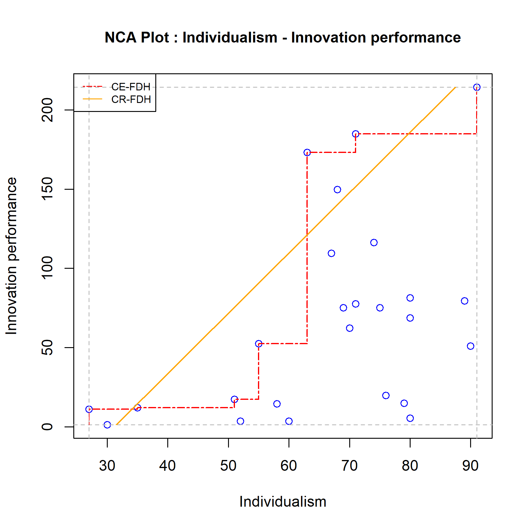
Figure 4.5: Example of a ceiling line robustness check: Comparing the results of two ceiling lines.
In this example the choice of the ceiling line is not obvious. As suggested in Dul (2020) a robustness check could consist of performing the analysis with both ceiling lines and comparing the results. The results for the CE-FDH ceiling line are \(d = 0.58\) and \(p = 0.002\), and for the CR-FDH ceiling line are \(d = 0.51\) and \(p = 0.003\). Given the researcher’s other choices (e.g., effect size threshold = 0.1; p value threshold = 0.05) the ceiling line robustness check consists of evaluating whether the researcher’s conclusion about the necessity hypothesis remains the same (robust result) or differs (fragile result). In this case both ceiling lines produce the same conclusion regarding necessity in kind: the necessity hypothesis is supported, which suggests that this is a robust result.
In the situation of a dichotomous necessary condition where the condition or the outcome (or both) have only two values, the only feasible ceiling line is the CE_FDH ceiling line. The CR_FDH ceiling line is not a plausible alternative as it does not fit the step-wise data pattern, and the results are already known: the CR_FDH effect size is half of the CE_FDH effect size, whereas the p values are the same. In this situation, the robustness check should exclude selecting another ceiling line.
Regarding necessity in degree the bottleneck tables (with outcome and conditions expressed as percentiles) shows that the results are more variable. For example, Figure ?? shows that for a “high” level of the outcome that can only be achieved by 25% of the cases (75th percentile), 32% of the cases (8 cases) cannot achieve the required level for the condition individualism when the CE-FDH line is used, whereas 20% of the cases (5 cases) cannot achieve when the CR-FDH line is used.
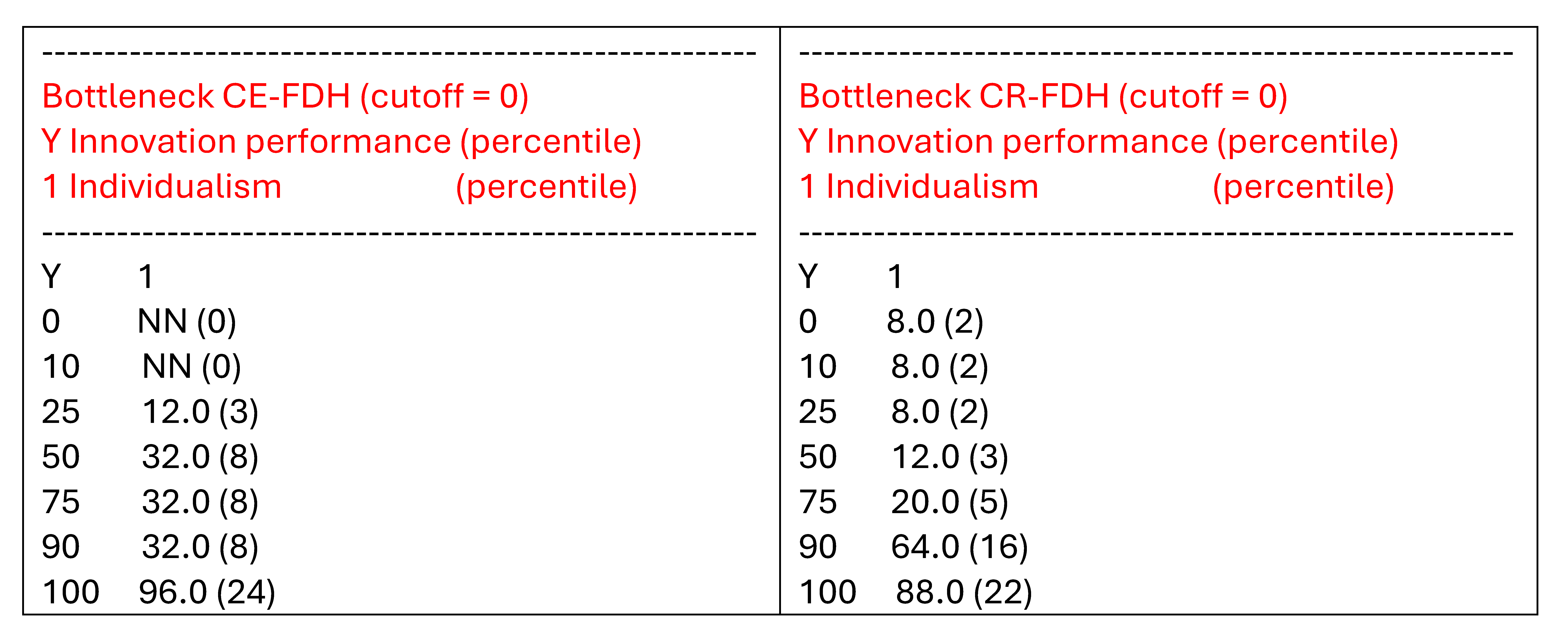
Figure 4.6: Bottleneck tables of for two ceiling lines.
4.4.2 Choice of the threshold level of the effect size
The researcher could also have made another choice for the effect size threshold level. If the threshold level is changed from the common 0.1 value (“small effect”) to a larger value of 0.2 (“medium effect”), the conclusion about necessity would not change. Since the observed effect size is verly large, the robustness check of effect size threshold suggests a robust result.
4.4.3 Choice of the threshold level of the p value
The researcher could also have made another choice for the p value threshold level. If the threshold level is changed from the common 0.05 value to a smaller value of 0.01, the conclusion about necessity would not change. Singe the estimated p values is very small, the robustness check of effect size threshold suggests a robust result.
4.4.4 Choice of the scope
Whereas regression analysis assumes that the variables of the regression model are unbounded (can have values between minus and plus infinity, see Section 4.5), NCA assumes that the variables in the necessity model are bounded (have minimum and maximum values). As a default the NCA selects the bounds based on the observed minimum and maximum values of the condition and the outcome to define the ‘empirical scope’. However, it is also possible to conduct NCA with a theoretically defined scope (‘theoretical scope’). The robustness of the result could be checked by selecting another plausible scope (‘theoretical scope’) than the default empirical scope, or when the original choice was a theoretical scope to select the empirical scope or a different theoretical scope. For example, the researcher may have selected the empirical scope for an analysis with variables measured with a Likert scale, but the scale’s minimum and maximum values are not used. Then the researcher can conduct a robustness check with a theoretical scope defined with the extreme values of the scale. Changing the scope for a larger theoretical scope generally results in a larger effect size. Therefore, such change may affect the researcher’s original conclusion that the hypothesis is rejected, but will not change an original conclusion that the hypothesis is supported. The latter is shown in Figure 4.7. The scatter plot has a theoretical scope that is larger than the empirical scope. The condition ranges from 20 to 100 and the outcome from 0 to 120. The effect size for the CE-FDH ceiling line has increased from \(d = 0.58\) (\(p = 0.002\)) to \(d = 0.61\) (\(p = 0.002\)). Changing a theoretical scope for a smaller scope generally results in a smaller effect size. Such change may affect the researcher’s original conclusion that the hypothesis is supported, but will not change an original conclusion that the hypothesis is rejected.
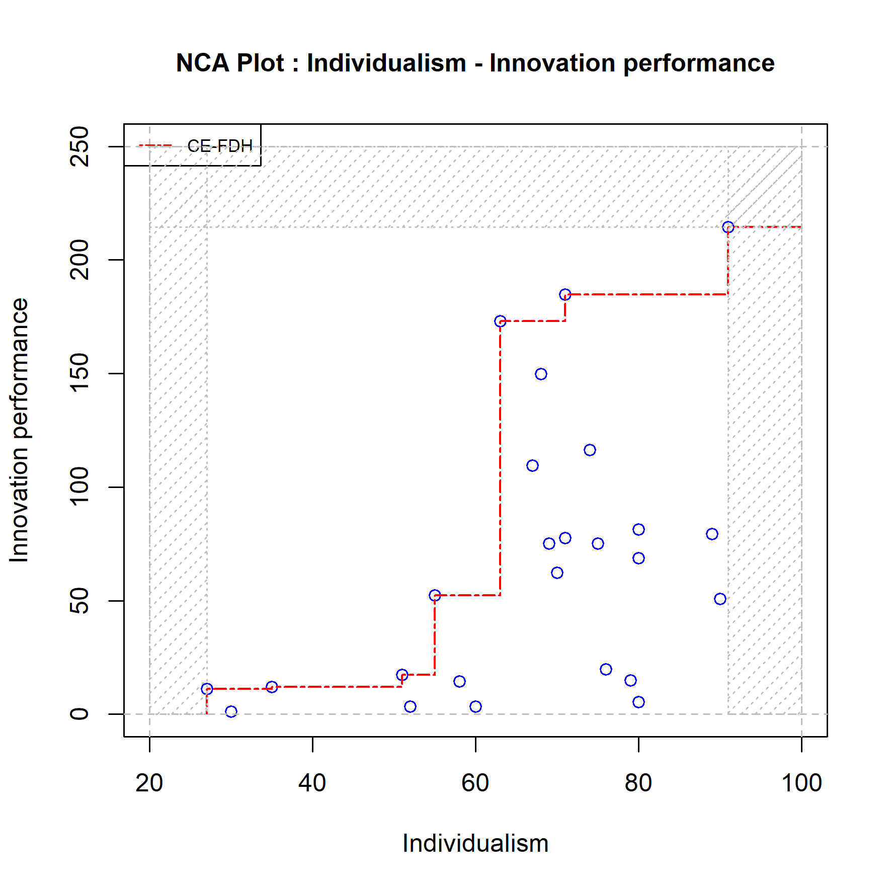
Figure 4.7: Example of a scope robustness check: Comparing the results with the empirical and the theoretical scope (difference is shaded).
When the researcher would have selected a theoretical scope for the analysis and changes that for a smaller theoretical scope, the effect size will be smaller and may also affect the researcher’s conclusion about the hypothesis from ‘rejected’ to ‘not rejected’.
4.4.5 Choice of outlier removal
A removal of outliers potentially has a large influence on the results as NCA results can be sensitive for outliers (see Section 3.8). Ceiling outliers (outliers that define the ceiling line) and scope outliers (outliers that define the scope) usually increase the effect size when removed. For example, in Figure 4.10 Finland is a potential ceiling outlier that increases the CE-FDH effect size from 0.58 (\(p = 0.002\)) to 0.62 (\(p = 0.001\)) and Mexico is a potential scope outlier that increases the effect size slightly. However, when an outlier is both a ceiling outlier and a scope outlier the effect may decrease. This applies to the potential outlier USA, where the effect size decreases from 0.58 (\(p = 0.002\)) to 0.52 (\(p = 0.012\)) when this potential outlier is removed.
For getting a first impression about the role of removing outliers two robustness checks can be done. In the first check the most influential single outlier (largest effect on the effect size if removed is selected, and this potential outlier is removed from the dataset. The potential outliers can be identified with the NCA software as follows:
The results are shown in Figure 4.8, where eff.or is the original effect size, eff.nw is the new effect size after removing the potential outlier, dif.abs and dif.rel are the absolute and relative differences between the new and original effect size and ‘ceiling’ and ‘scope’ indicate whether the potential outliers is a ceiling outlier or a scope outlier (or both). It turns out the USA is the largest outlier. When this case is removed from the dataset the NCA results are changed as indicated above.
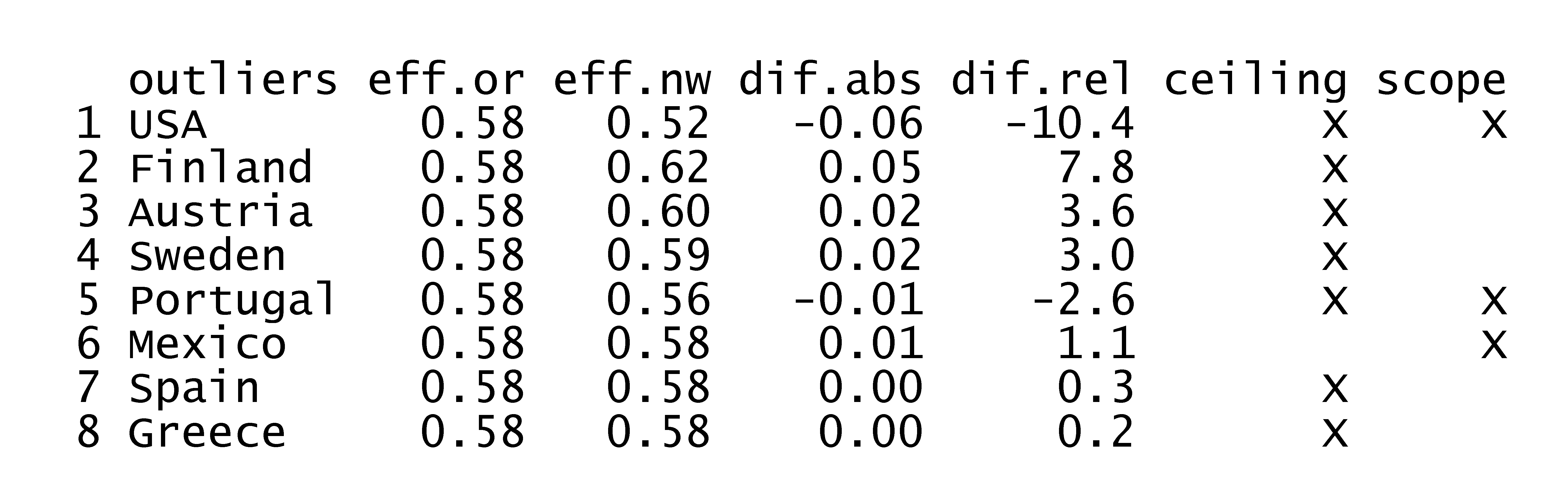
Figure 4.8: The influence of removing a single potential outlier on the effect size.
In the second check, multiple outliers (for example a set of two) are selected that have the largest influence on the effect size when removed as a set. This outlier analysis can be initiated as follows:
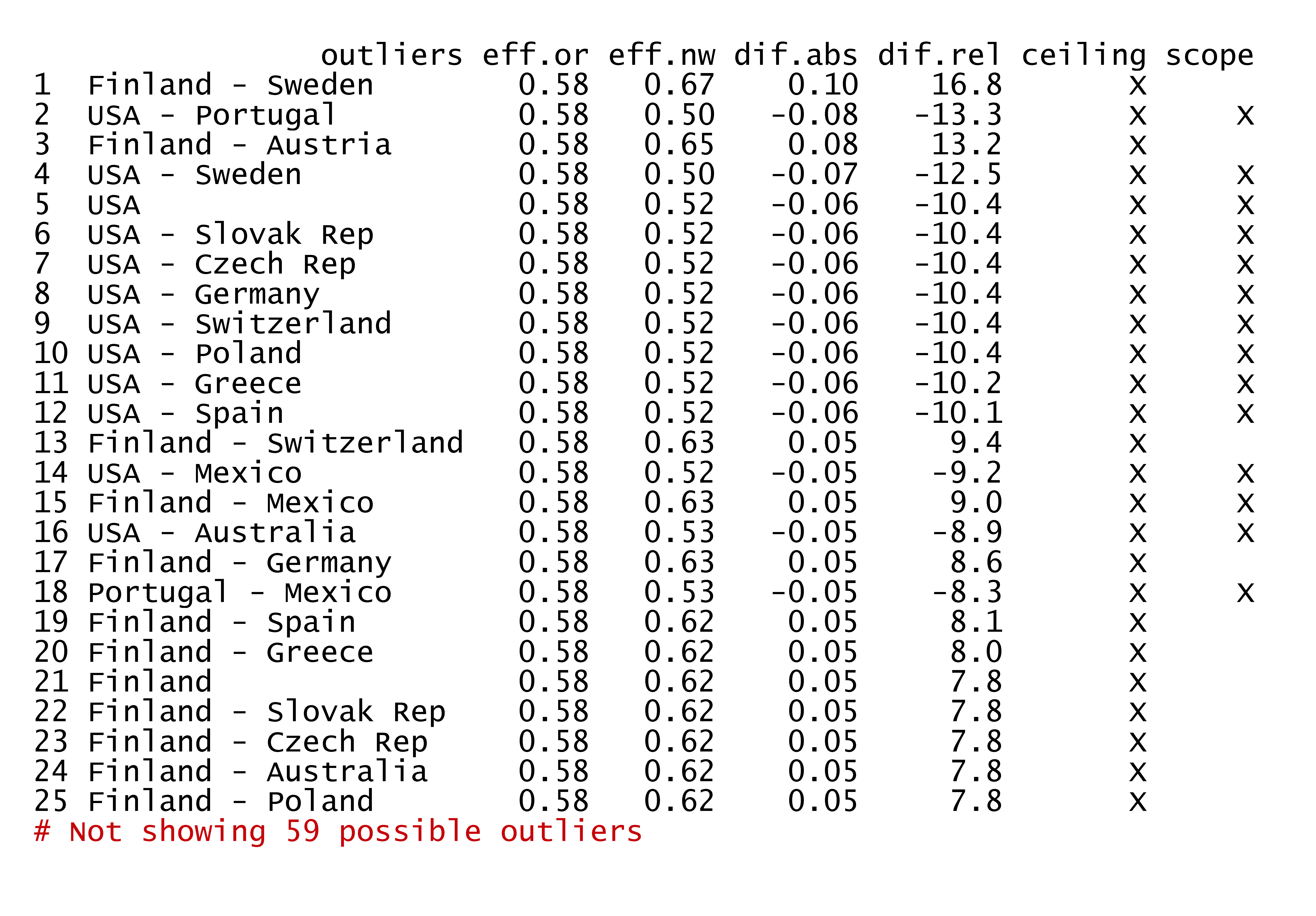
Figure 4.9: The influence of removing two potential outliers on the effect size.
The results show that the set ‘Finland-Sweden’ is the most influential outlier duo. If this duo is removed from the dataset, the effect size increases and the p value reduces.
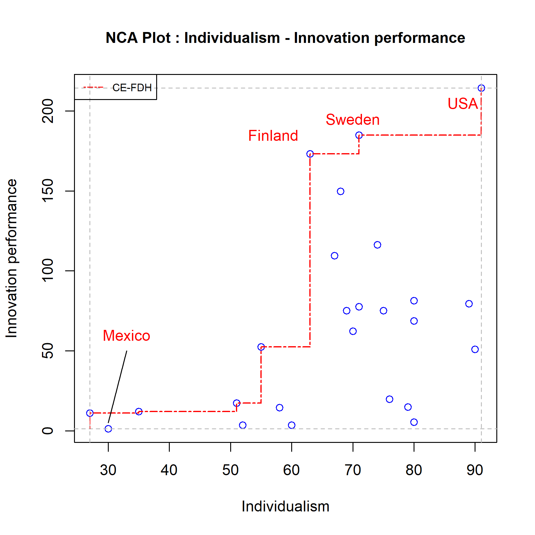
Figure 4.10: Potential outliers. Mexico = potential scope outlier; Finland, Sweden = potential ceiling outliers; USA = potential scope and ceiling outlier. USA is the most influential single outlier. Finland - Sweden is the most influential combination of multiple (two) outliers.
If this crude outlier approach with removing a single most influential outlier and aset of multiple most influential outliers does not change the conclusions, the results can be considered robust. Note, however, that a careful consideration is needed about an outlier decision: What are potential outliers, what are reasons of removing or not removing them (see decision tree about outliers in Section 3.8), and what is their influence on the effect size. Outliers are usually only removed when they are erroneous (measurement error or sampling error) or when they are exceptional (very large influence on the effect size when removed). In the current example, the influence of removing potential outliers is relatively modest; keeping them seems to be the most appropriate approach.
4.4.6 Choice of target outcome
The last robustness check explores the stability of the bottleneck analysis in terms of the number of bottleneck cases (that cannot achieve the target outcome because the condition is not satisfied) when the target outcome is mildly changed. For example, when the original target outcome is 75% (percentile) what is the influence on the percentage and number of bottleneck cases when the target outcome is somewhat lower (70%) or higher (80%).
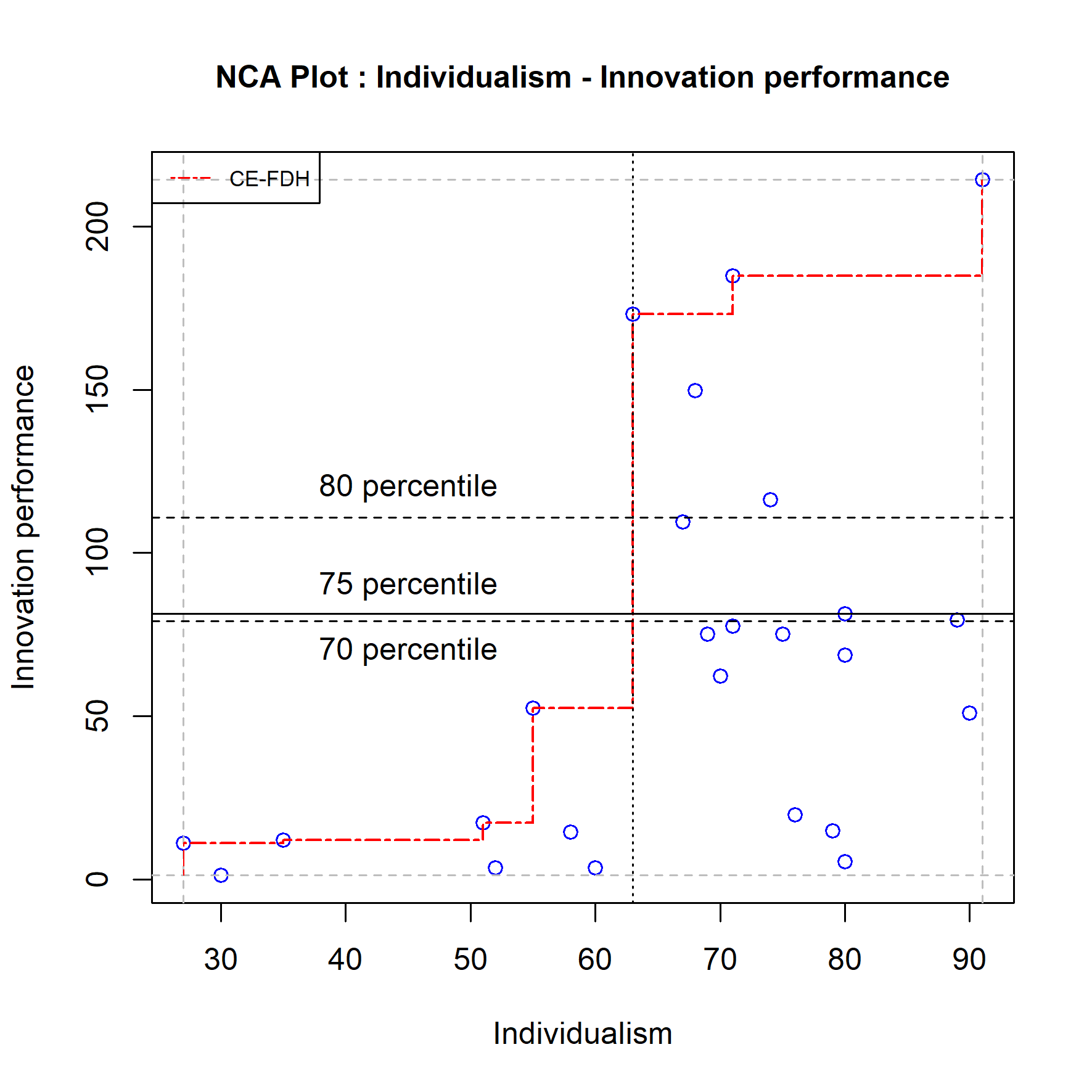
Figure 4.11: The effect of changing the target outcome from 75 percentile to 70 and 80 percentile.
Figure 4.11 shows that for each of these levels of the outcome the required minimum level of the condition is 63. Eight cases (32%) have not reached that level of the condition, which makes them bottleneck cases. The number of bottleneck cases does not change with minor changes of the target outcome.
4.4.7 Robustness table
The results the robustness checks can be summarized in a NCA robustness table (4.1) where the original NCA results are compared with the results when different, also feasible choices are made. The first row shows the original results, and the next rows give the results after changes are explored. The nine changes: ceiling line change, d threshold change, p threshold change, scope change, single outlier removal, multiple outlier removal, target lower, and target higher. For checking the robustness of necessity in kind, effect size, p value, and conclusion about necessity (assuming theoretical support) are displayed. For checking the robustness of necessity in degree the percentage (%) and number (#) of bottleneck cases that are unable to achieve the required level of the condition for a selected target level of the outcome are shown. The NCA robustness table shows that the original results of this example are robust.
| Robustness check | Effect size | p value | Necessity | Bottlenecks(%) | Bottlenecks(#) |
|---|---|---|---|---|---|
| Individualism | |||||
| Original | 0.58 | 0.100 | no | 32 | 8 |
| Ceiling change | 0.51 | 0.100 | no | 20 | 5 |
| d threshold change | 0.58 | 0.100 | no | 32 | 8 |
| p threshold change | 0.58 | 0.100 | no | 32 | 8 |
| Scope change | 0.61 | 0.100 | no | 32 | 8 |
| Single outlier removal | 0.52 | 0.100 | no | 33.3 | 8 |
| Multiple outlier removal | 0.67 | 0.100 | no | 34.8 | 8 |
| Target lower | 0.58 | 0.100 | no | 32 | 8 |
| Target higher | 0.58 | 0.100 | no | 32 | 8 |
The NCA robustness table for a specific necessity relationship with one condition and one outcome can be produced with the following code that makes use of three functions: nca_robustness_table_general, nca_robustness_checks_general, and get_outliers. The R code for these functions can be found in Sections 7.4.1, 7.4.2, and 7.4.3, respectively.
# General robustness table for a single necessity relationship.
library(NCA)
source("nca_robustness_table_general.R")
source("nca_robustness_checks_general.R")
source("get_outliers.R")

# Example (nca.example with Western countries)
data(nca.example)
data <- nca.example
data <- data[-c(14,22,26),] #exclude non-Western countries
conditions <- "Individualism"
outcome <- "Innovation performance"
bottleneck.y <- "percentile"
plots <- FALSE # do not show scatter plots

# Define original analysis
define_check <- function(
    name,
    ceiling = "ce_fdh", # original
    d_threshold = 0.1, # original
    p_threshold = 0.05, # original
    scope = NULL, # original
    outliers = 0, # original
    target_outcome = 75 # original
) {
  list(
    name = name,
    ceiling = ceiling,
    d_threshold = d_threshold,
    p_threshold = p_threshold,
    scope = scope,
    outliers = outliers,
    target_outcome = target_outcome
  )
}

# Define robustness checks (differences with Original)
checks <- list(
  define_check("Original"),
  define_check("Ceiling change", ceiling = "cr_fdh"),
  define_check("d threshold change", d_threshold = 0.2),
  define_check("p threshold change", p_threshold = 0.01),
  define_check("Scope change", scope = list(c(20, 100, 0, 250))),
  define_check("Single outlier removal", outliers = 1),
  define_check("Multiple outlier removal", outliers = 2),
  define_check("Target lower", target_outcome = 80),
  define_check("Target higher", target_outcome = 90)
)

# Conduct robustness checks and produce robustness table
results <- nca_robustness_table_general(
  data = data,
  conditions = conditions,
  outcome = outcome,
  ceiling = ceiling,
  scope = scope,
  d_threshold = d_threshold,
  p_threshold = p_threshold,
  outliers = outliers,
  bottleneck.y = bottleneck.y,
  target_outcome = target_outcome,
  plots = plots,
  checks = checks
)

# View results
print(results)
4.5 Combining NCA with regression analysis
4.5.1 Introduction
Regression is the mother of all data analyses in the social sciences. It was invented more than 100 years ago when Francis Galton (Galton, 1886) quantified the pattern in the scores of parental height and child height (see Figure 4.12 showing the original graph).
Figure 4.12: Francis Galton’s (1886) graph with data on Parent height (‘mid-parents height’) and Child height (‘Adult children height’).
In Figure 4.13 Galton’s data are shown in two \(XY\) scatter plots.
Figure 4.13: Scatter plots of the relationship between Parent height (\(X\)) and Child height (\(Y\)) (after Galton (1886). A. With a regression line. B. With a ceiling line.
Galton drew lines though the middle of the data for describing the average trend between Parental height and Child height: the regression line (Figure 4.13 A). For example, with a Parent height of 175 cm, the estimated average Child height is about 170 cm. Galton could also have drawn a line on top of the data for describing the necessity of Parent height for Child height: the ceiling line (Figure ?? B). For example, with a Parent height of 175 cm, the estimated maximum possible Child height is about 195 cm. But Galton did not draw a ceiling line, and the social sciences have adopted the average trend line as the basis for many data analysis approaches. Regression analysis has developed over the years and many variants exist. The main variant is Ordinary Least Squares (OLS) regression. It is used for example in Simple Linear Regression (SLR), Multiple Linear Regression (MLR), path analysis, variance-based Structural Equation Modeling (SEM) and Partial Least Squares Structural Equation Modeling (PLS-SEM). In this section I compare OLS regression with NCA.
4.5.2 Logic and theory
OLS regression uses additive, average effect logic. The regression line (Figure 4.13 A) predicts the average \(Y\) for a given \(X\). Because the cases are scattered, for a given \(X\) also higher and lower values of \(Y\) than the average value of \(Y\) are possible. With one \(X\) (Simple Linear Regression), \(Y\) is predicted by the regression equation is:
\[\begin{equation} \tag{4.1} Y = β_0 + β_1 X + ɛ(X) \end{equation}\]
where \(β_0\) is the intercept of the regression line, \(β_1\) is the slope of the regression line, and \(ɛ(X)\) is the error term representing the scatter around the regression line for a given \(X\). The slope of the regression line (regression coefficient) is estimated by minimizing the squared vertical distances between the observed \(Y\)-values and the regression line (‘least squares’). The error term includes the effect of all other factors that can contribute to the outcome \(Y\).
For the parent-child data, the regression equation is \(Y = 57.5 + 0.64 X + ɛ(X)\). OLS regression assumes that on average \(ɛ(X) = 0\). Thus, when \(X\) (Parent height) is 175 cm, the estimated average Child height is about 170 cm. In contrast NCA’s C-LP ceiling line is defined by \(Y_c = -129 + 1.85 X\). Thus, when \(X\) (Parent height) is 175 cm, the estimated maximum possible Child height is about 195 cm. Normally, in NCA the ceiling line is interpreted inversely (e.g., in the bottleneck table): \(X_c = (Y_c + 129)/1.85\) indicating, while assuming a non-decreasing ceiling line, that a minimum level of \(X = X_c\) is necessary (but not sufficient) for a target level of \(Y =Y_c\). When parents wish to have a child of 200 cm it is necessary (but not sufficient) that their Parent height is at least about 177 cm.
To allow for doing statistical tests with OLS, it is usually assumed that the error term for a given \(X\) is normally distributed (with average value 0): cases close to the regression line for the given \(X\) are more likely than cases far from the regression line. The normal distribution is unbounded, hence very high or very low values of \(Y\) are possible, though not likely. This implies that any high value of \(Y\) is possible. Even without the assumption of the normal distribution of the error term, a fundamental assumption of OLS is that the \(Y\) value is unbounded (Berry, 1993). Thus, very large child heights (e.g., 300 cm) are theoretically possible in OLS, but unlikely. This assumption contradicts NCA’s logic in which \(X\) and \(Y\) are presumed bounded. \(X\) puts a limit on \(Y\) and thus there is a border represented by the ceiling line. The limits can be empirically observed in the sample (e.g., the height of the observed tallest person in the sample is 205 cm) for defining NCA’s empirical scope or can be theoretically defined (e.g., the height of the ever-observed tallest person of 272 cm) for defining the NCA’s theoretical scope.
Additivity is another part of regression logic. It is assumed that the terms of the regression equation are added. Next to \(X\), the error term is always added in the regression equation. Possibly also other \(X\)’s or combination of \(X\)’s are added in the regression equation (multiple regression, see below). This means that the terms that make up the equation can compensate for each other. For example, when \(X\) is low, \(Y\) can still be achieved when other terms (error term or other \(X\)’s) give a higher contribution to \(Y\). The additive logic implies that for achieving a certain level of \(Y\), no \(X\) is necessary. This additive logic contradicts NCA’s logic that \(X\) is necessary: \(Y\) cannot be achieved when the necessary factor does not have the right level, and this absence of \(X\) cannot be compensated by other factors.
Results of a regression analysis are usually interpreted in terms of probabilistic sufficiency. A common probabilistic sufficiency-type of hypotheses is ‘\(X\) likely increases \(Y\)’ or ‘\(X\) has an average positive effect on \(Y\)’. Such hypothesis can be tested with regression analysis. The hypothesis is considered to be supported if the regression coefficient is positive. Often, it is then suggested that \(X\) is sufficient to produce an increase the likelyhood of the outcome \(Y\). The results also suggest that a given \(X\) is not necessary for producing the outcome \(Y\) because other factors in the regression model (other \(X\)’s and the error term) can compensate for the absence of a low level of \(X\).
4.5.3 Data analysis
Most regression models include more than one \(X\). The black box of the error term is opened and other \(X\)’s are added to the regression equation (Multiple Linear Regression - MLR), for example:
\[\begin{equation} \tag{4.2} Y = β_0 + β_1 X_1 + β_2 X_2 + \epsilon_X \end{equation}\]
where \(β_1\) and \(β_2\) are the regression coefficients. By adding more factors that contribute to \(Y\) into the equation, \(Y\) is predicted for given combinations of \(X\)’s,and a larger part of the scatter is explained. R\(^2\) is the amount of explained variance of a regression model and can have values between 0 and 1. By adding more factors, usually more variance is explained resulting in higher values of R\(^2\).
Another reason to add more factors is to avoid ‘omitted variable bias’. This bias is the result of not including factors that correlate with \(X\) and \(Y\), which causes in biased estimations of the regression coefficients. Hence, the common standard of regression is not the simple OLS regression with one factor, but multiple regression with many factors including control variables to reduce omitted variable bias. By adding more relevant factors, the prediction of \(Y\) becomes better and the risk of omitted variable bias is reduced. Adding factors in the equation is not just adding new factors (\(X\)). Some factors may be combined such as squaring a factor (\(X^2\)) to represent a non-linear effect of \(X\) on \(Y\), or taking the product of two factors \((X_2 * X_2)\) to represent the interaction between these factors. Such combination of factors are added as a separate terms into the regression equation. Also, other regression-based approaches such as SEM and PLS-SEM include many factors. In SEM models factors are ‘latent variables’ of the measurement model of the SEM approach.
A study by Bouquet & Birkinshaw (2008) is an example of the prediction of an average outcome using MLR by adding many terms including combined factors in the regression equation. This highly cited article in the Academy of Management Journal studies multinational enterprises (MNE’s) to predict how subsidiary companies gain attention from their headquarters (\(Y\)). They use a multiple regression model with 25 terms (\(X\)’s and combination of \(X\)’s) and an ‘error’ term \(ɛ\). With the regression model the average outcome (average attention) for a group of cases (or for the theoretical ‘the average case’) for given values of the terms can be estimated. The error term represents all unknown factors that have a positive or negative effect on the outcome but are not included in the model, assuming that the average effect of the error term is zero. \(β_0\) is a constant and the other \(β_i\)’s are the regression coefficients of the terms, indicating how strong the term is related to the outcome (when all other terms are constant). The regression model is:
\(Attention = \\ β_0 \\ + β_1\ Subsidiary\ size \\ + β_2\ Subsidiary\ age \\ + β_3\ (Subsidiary\ age)^2 \\ + β_4\ Subsidiary\ autonomy \\ + β_5\ Subsidiary\ performance \\ + β_6\ (Subsidiary\ performance)^2 \\ + β_7\ Subsidiary\ functional\ scope \\ + β_8\ Subsidiary\ market\ scope \\ + β_9\ Geographic\ area\ structure \\ + β_{10}\ Matrix\ structure \\ + β_{11}\ Geographic\ scope \\ + β_{12}\ Headquarter\ AsiaPacific\ parentage \\ + β_{13}\ Headquarter\ NorthAmerican\ parentage \\ + β_{14}\ Headquarter\ subsidiary\ cultural\ distance \\ + β_{15}\ Presence\ of\ MNEs\ in\ local\ market \\ + β_{16}\ Local\ market\ size \\ + β_{17}\ Subsidiary\ strength\ within\ MNE\ Network \\ + β_{18}\ Subsidiary\ initiative\ taking \\ + β_{19}\ Subsidiary\ profile\ building \\ + β_{20}\ Headquarter\ subsidiary\ geographic\ distance \\ + β_{21}\ (Initiative\ taking * Geographic\ distance) \\ + β_{22}\ (Profile\ building * Geographic\ distance) \\ + β_{23}\ Subsidiary\ downstream\ competence \\ + β_{24}\ (Initiative\ taking * Downstream\ competence) \\ + β_{25}\ (Profile\ building * Downstream\ competence) \\ + \epsilon\)
The 25 terms of single and combined factors in the regression equation explain 27% of the variance (R\(^2\) = 0.27). Thus, the error term (representing the not included factors) represent the other 73% percent (unexplained variance). Single terms predict only a small part of the outcome. For example, ‘subsidiary initiative taking’ (term 18) is responsible for 2% to the explained variance.
The example shows that adding more factors makes the model more complex and less understandable and therefore less useful in practice. The contrast with NCA is large. NCA can have a model with only one factor that perfectly explains the absence of a certain level of an outcome when the factor is not present at the right level for that outcome. Whereas regression models must include factors that correlate with other factors and with the outcome to avoid biased estimation of the regression coefficient, NCA’s effect size for a necessary factor is not influenced by the absence or presence of other factors in the model. This is illustrated with and example about the effect of a sales person’s personality on sales performance using data of 108 cases (sales representatives from a large USA food manufacturer) obtained with The Hogan Personality Inventory (HPI) personality assessment tool for predicting organizational performance (Hogan & Hogan, 2007). Details of the example are in Dul, Hauff, et al. (2021). The statistical descriptives of the data (mean, standard deviation, correlation) are shown in Figure 4.14 A. Ambition and Sociability are correlated with \(Y\) as well as each other. Hence, if one of them is omitted from the model the regression results may be biased.

Figure 4.14: Example of the results of a regression analysis and NCA. Effect of four personality traits of sales persons on sales performance. A. Descriptive statistics. B. Results of regression analysis and NCA for two different models. Data from Hogan & Hogan (2007)
The omission of one variable is shown in Figure 4.14 B, middle column. The full model (Model 1) includes all four personality factors. The regression results show that Ambition and Sociability have positive average effects on Sales performance (regression coefficients 0.13 and 0.16 respectively, and Learning approach has a negative average effect on Sales performance (regression coefficient -0.11). Interpersonal sensitivity has virtually no average effect on Sales performance (regression coefficient 0.01). The p values for Ambition and Sociability are relatively small. Model 2 has only three factors because Sociability is omitted. The regression results show that the regression coefficients of all three remaining factors have changed. The regression coefficient for Ambition has increased to 0.18, and the regression coefficients of the other two factors have minor differences (because these factors are less correlated with the omitted variable). Hence, in a regression model that is not correctly specified because factors that correlate with factors that are included in the model and with the outcome are not included, the regression coefficients of the included factors may be biased (omitted variable bias). However, the results of the NCA analysis does not change when a variable is omitted (Figure 4.14 B, right column). This means that an NCA model does not suffer from omitted variable bias.
4.5.4 How to combine NCA and regression
Regression and NCA are fundamentally different and complementary. A regression analysis can be added to a NCA study to evaluate the average effect of the identified necessary condition for the outcome. However, the researcher must then include all relevant factors, also those that are not expected to be necessary, to avoid omitted variable bias, and must obtain measurement scores for these factors. When NCA is added to a regression study, not much extra effort is required. Such regression study can be a multiple regression analysis, or the analysis of the structural model of variance based structural equation modeling (SEM), Partial Least Squares structural equation modeling (PLS-SEM) or another regression technique. If a theoretical argument is available for a factor (indicator or latent construct) being necessary for an outcome, any factor that is included in the regression model (independent variables, moderators, mediators) can also be treated as a potential necessary condition that can be tested with NCA. This could be systematically done:
For all factors in the regression model that are potential necessary conditions.
For those factors that provide a surprising result in the regression analysis (e.g., in terms of direction of the regression coefficient, see below the situation of disparate duality) to better understand the result.
For those factors that show no or a limited effect in the regression analysis (small regression coefficient) to check whether such ‘unimportant’ factors on average still may be necessary for a certain outcome.
For those factors that have a large effect in the regression analysis (large regression coefficient) to check whether an ‘important’ factor on average may also be necessary.
When adding NCA to a regression analysis more insight about the effect of \(X\) on \(Y\) can be obtained.
Figure 4.15 shows a example of a combined NCA and simple OLS regression analysis.
Figure 4.15: Example of interpretation of findings from regression analysis and NCA
\(X\) and \(Y\) are related with correlation coefficient 0.58. The data may be interpreted as an indication of a necessity relationship, an indication of an average effect relationship, or both. The average relationship is illustrated with a green OLS regression line with intercept 0.66 and slope 0.9 (p < 0.001). The ceiling line (C-LP) is illustrated with the dashed blue with intercept 1.1 and slope 1.0 (effect size d = 0.24; p < 0.001). According the ceiling line, for an outcome value \(Y = 1.3\), a minimum level of the condition of \(X = 0.15\) is necessary. According to the vertical line \(X = 0.15\), the average value of the outcome for this value the condition is \(Y = 0.8\). In other words, for a given value of \(X\) (e.g., \(X =0.15\)), NCA predicts the maximum possible value of \(Y\) (\(Y = 1.3\)), whereas OLS regression predicts the average value of \(Y\) (\(Y = 0.8\)). OLS regression does not predict a maximum value of \(Y\). Regression analysis assumes that any value of \(Y\) is possible. Also very high values of \(Y\), up to infinity, are possible, but unlikely. The horizontal line \(Y = 1.3\) not only intersects the ceiling line, showing the required level of \(X = 0.15\) that all cases must have satisfied to be able to reach \(Y = 1.3\), but also the OLS regression line, showing that the average outcome \(Y = 1.3\) is obtained when \(X = 0.72\). The vertical line \(X = 0.72\) intersects the ceiling line at \(Y = 1.9\), showing that this outcome level is maximally possible when the condition level \(X = 0.72\).
In this example the regression line has the same direction as the ceiling line. There is a positive average effect and a ‘positive’ necessity effect (high level of \(X\) is necessary for high level of \(Y\)). I call this situation: ‘commensurate duality’. Commensurate duality also applies when both lines have negative slopes. It is also possible, but less common that the slope of the ceiling line is positive and the slope of the regression line is negative. In this situation there is a negative average effect and a ‘positive’ necessity effect. A high level of \(X\) is necessary for high level of \(Y\), but increasing \(X\) on average reduces \(Y\). This can occur when a relatively high number of cases are in the lower right corner of the scatter plot (cases with high \(X\) that do not reach high \(Y\)). The situation when both lines have opposite slopes is called ‘disparate duality’. A third situation is possible that there is no significant average effect and yet a significant necessity effect, or the other way around. I call this situation ‘impact duality’. The word ‘duality’ refers to a data interpretation battle. Should the observed data pattern be describe with regression analysis, NCA or both? The answer depends on the researcher’s theory. When a conventional theory with additive/average effect logic is used, regression analysis ensures theory-method fit. When a necessity theory is used, NCA ensures theory-method fit. When a conventional theory and a necessity theory are both used (e.g., in an ‘embedded necessity theory,’ see Bokrantz & Dul, 2023 and see Chapter 2) both methods should be used to ensure theory-method fit. Hence, it depends on the underlying theory what method(s) should be selected to analyse the data.
4.5.5 What is the same in NCA and regression?
I showed that regression has several characteristics that are fundamentally different from the characteristics of NCA. Regression is about average trends, uses additive logic, assumes unbounded \(Y\) values, is prone to omitted variable bias, needs control variables, and is used for testing sufficiency-type of hypotheses, whereas NCA is about necessity logic, assumes limited \(X\) and \(Y\), is immune for omitted variable bias, does not need control variables, and is used for testing necessity hypotheses.
However, NCA and regression also share several characteristics. Both NCA and regression are variance-based approaches and use linear algebra (although NCA can also be applied with the set theory approach with Boolean algebra; see Section 4.7 on NCA and QCA). Both methods need good (reliable and valid) data without measurement error, although NCA may be more prone to measurement error. For statistical generalization from sample to population both methods need to have a probability sample that is representative for the population, and having larger samples usually give more reliable estimations of the population parameters, although NCA can handle small sample sizes. Additionally, for generalization of the findings of a study both methods need replications with different samples; a one-shot study is not conclusive. Both methods cannot make strong causal interpretations when observational data are used; then at least also theoretical support is needed. When null hypothesis testing is used in both methods, such tests and the corresponding p values have strong limitations and are prone to misinterpretations; a low p value only indicates a potential randomness of the data and is not a prove of the specific alternative hypothesis of interest (average effect, or necessity effect).
When a researcher uses NCA or OLS, these common fundamental limitations should be acknowledged. When NCA and OLS are used in combination the fundamental differences between the methods should be acknowledged. It is important to stress that one method is not better than the other. NCA and OLS are different and address different research questions. To ensure theory-method fit, OLS is the preferred method when the researcher is interested in an average effect of \(X\) on \(Y\), and NCA is the preferred method when the researcher is interested in the necessity effect of \(X\) on \(Y\).
4.6 Combining NCA with (PLS-)SEM
One of the most common applications of combining NCA with a regression-based method is the use of NCA in the context of Partial Least Squares - Structural Equation Modeling (PLS-SEM). The reason for this popularity may be two-fold.
Leading PLS-SEM proponents introduced NCA as a methodological enrichment of PLS-SEM, and provided specific recommendations (Richter, Schubring, et al., 2020; Richter et al., 2022; Richter, Hauff, Ringle, et al., 2023) and extensions (Hauff et al., 2024; Sarstedt et al., 2024) on how to use NCA in combination with PLS-SEM.
A basic version of the NCA software became part of a popular software package for conducting PLS-SEM (SmartPLS, see Section 7.1.2).
NCA has also been applied in combination with other types of SEM such as the classical covariance-based SEM (CB-SEM).
A SEM model consists of two parts. The measurement model defines how latent variables are represented by measured indicators. A latent variable is an unobserved construct that is derived from observed indicators. The structural model specifies how the latent variables are related to each other.
In both PLS-SEM and CB-SEM, latent variable scores can be obtained and used for further analysis. However, the estimation approach differs. PLS-SEM uses partial least squares to estimate latent variable scores as weighted composites of indicators and to maximize the explained variance in the dependent variables. CB-SEM estimates model parameters based on the covariance matrix, using techniques such as maximum likelihood or generalized least squares. Latent variable scores are not directly estimated in the model fitting process, but can be computed afterward if needed (e.g., as factor scores).
Combining NCA with SEM involves using the estimated scores of the latent variables as input for NCA. This allows researchers to examine whether a relationship between two latent variables are not only related in terms of probabilistic sufficiency (as modeled in SEM) but also in terms of necessity, assuming a theoretical rationale exists. In NCA, latent variables from the structural model can take the role of condition or outcome to study necessity relationships.
All guidelines for applying NCA in general (see Sections 1.7 and 1.8) also apply to combining NCA with SEM.
4.6.1 Steps for conducting NCA with SEM
Figure 4.16 shows a flowchart for conducting NCA in combination with SEM.
Figure 4.16: Flowchart for conducting NCA in combination with Structural Equation Modeling (SEM).
Below the steps are discussed in detail and an example is given about how to use NCA with PLS-SEM. Since SEM terminology about ‘indicators’, ‘weights’, ‘latent variables’ and ‘rescaling’ varies across the SEM literature, the following terminology is used in this book:
Terminology
General:
Rescaling: normalization or standardization of original scores.
Normalization (or min-max normalization): rescaling of scales with new minimum and maximum values (e.g., 0-1 or 0-100).
Standardization: Rescaling of observed scale values based on the their probability distribution. (z-score)
Indicator:
Indicator (variable). A manifest/measured variable linked to a latent variable.
Indicator score. The value of an indicator.
Raw indicator score. The value of the indicator measured on a scale. The scale usually has minimum and maximum values, e.g., Likert scale ranging from 1-5 or 1-7.
Normalized indicator score. The value of an indicator after min-max normalization of the raw indicator score (e.g., 0-1 scale or percentage scale 0-100).
Standardized indicator score. The value of an indicator after standardization of the raw indicator (z-score: rescaled such that the mean = 0 and standard deviation = 1).
Original indicator score. The indicator that is used as input for the SEM model (raw score or standardized score), which can be raw or standardized depending on the estimation settings.
Weight and loading:
(Indicator) weight. In PLS-SEM, the extent to which an indicator contributes to the latent variable score (as part of a weighted composite).
Standardized indicator weight. Indicator weight using standardized indicators.
Estimated indicator weight. In PLS-SEM, the estimated coefficient that multiplies an indicator to construct the latent variable score.
Factor loading. In CB-SEM, the strength of indicator–latent variable relationships.
Latent variable:
- Latent variable. An unobserved construct linked to multiple indicators.
Latent variable score. The value of a latent variable, calculated as a linear combination (weighted sum) of indicator scores.
Standardized latent variable score. The value of a latent variable obtained by linear combination (weighted sum) of standardized indicator scores (z -score).
Unstandardized latent variable score. The value of a latent variable expressed in the scale of the original indicators (commonly raw original scores).
Normalized unstandardized latent variable score. Unstandardized latent variable score after normalization.
4.6.1.1 Step 1: Theorize probabilistic and necessity relationships
The first step is a fundamental step for any combined NCA and SEM study. An NCA-SEM study implies that the relationships between the variables are considered from two different causal perspectives: probabilistic sufficiency (SEM) and necessity (NCA). Both SEM and NCA require that the study starts with formulating theoretical expectations about the relationship (e.g., hypotheses). According to SEM, all relationships between latent variables in the structural model are considered probabilistic sufficiency relationships. According to NCA all, a few, or none of the relationships can be hypothesized as necessity relationships as well. Each necessity relationship between latent variables should be theoretically justified (see Section 2.2). The theoretical justification of applying these different causal lenses to the structural model is essential (Dul, 2024a). A theory that includes one or more necessity relationships in addition to probabilistic sufficiency relationships is called an ‘embedded necessity theory’ (Bokrantz & Dul, 2023). The latent variables of a structural model can have two different roles. A ‘predictor’ variable (independent variable; ‘condition’ in NCA) explains or predicts a ‘predicted’ variable (dependent variable; outcome in NCA). For example, when in a structural model a latent variable \(M\) mediates the relationship between \(X\) and \(Y\), then \(M\) has two different roles. For the \(X\)-\(M\) relationship \(X\) is the predictor and \(M\) is the predicted variable, and for the \(M\)-\(Y\) relationship \(M\) is the predictor and \(Y\) the predicted variable. When a relationship is (also) considered a necessity relationship, NCA calls the predictor variable the ‘condition’ and the predicted variable the ‘outcome’.
4.6.1.2 Step 2: Conduct SEM
Conducting SEM assumes that data are available on observed indicators that are used to represent latent variables. SEM involves specifying a measurement model, which defines the relationships between indicators and latent variables, and a structural model, which specifies the relationships between latent variables. The complete model is then estimated using a chosen algorithm (e.g., PLS-SEM or CB-SEM). NCA is not part of the SEM estimation process itself, but it uses latent variable scores obtained from SEM as input for its own analysis. Therefore, it is important that the analyst ensures that the latent variable scores extracted from the SEM model are valid, reliable, and interpretable. Recommendations for good SEM practices are available in the literature and are not discussed here. Both commercial and open-source software tools are available to conduct SEM.
4.6.1.3 Step 3: Extract latent variable scores
The latent variable scores obtained from the SEM model serve as input for NCA. During SEM estimation, latent variable scores are often standardized (z-scores), resulting in scores with a mean of 0 and standard deviation of 1. Although NCA results are invariant to affine transformations (such as standardization or linear rescaling), it is recommended for purposes of interpretation to first unstandardize the latent variable scores, and then, if desired, apply normalization (e.g., min-max scaling). Unstandardized latent variable scores (see Step 3a, if needed) are expressed on a scale that is directly related to the original indicator scale, provided that the same measurement scale was used for all indicators of the latent construct. This allows for more meaningful interpretation of the NCA results, especially when discussing real-world implications and when results are discussed in terms of necessity ‘in degree’ with specified levels of \(X\) and \(Y\). Note that not all SEM software packages offer the option to extract unstandardized latent variable scores, particularly in CB-SEM, where latent scores are not estimated by default. Below is an example showing how to convert standardized scores back to unstandardized scores when needed. When all unstandardized latent variable scores are derived from indicators measured on the same scale (i.e., with identical minimum and maximum values), normalization is not required. However, if latent variables have different scales, min-max normalization is recommended (see Step 3b). This ensures that the latent variable scores are comparable, which is particularly important in later steps (e.g., Step 5: producing a BIPMA).
A common approach to min-max normalization is to rescale scores to a 0–100 range, allowing latent variable scores to be interpreted as percentages of their original scale range. Alternatively, rescaling to a 0–1 range can be used, which is often more convenient for NCA, as it yields a scope of 1. However, this is optional and not required for the validity of NCA results.
4.6.1.4 Step 4: Conduct NCA
The unstandardized and possibly normalized latent variable scores are input to NCA. In the first part of the analysis the hypothesized relationships are tested for ‘necessity in kind’, which is the qualitative statement that \(X\) is necessary for \(Y\) without specifying levels of \(X\) and \(Y\) other than absence/presence or low/high. The observed effect size \(d\) and p value are compared with their threshold values (e.g., \(d\) = 0.10; p = 0.05) that are set by the researcher to decide if a predictor variable is necessary for a predicted variable, as suggested by the hypothesis.
In the second part, identified necessary conditions are selected for a the bottleneck analysis for ‘necessity in degree’, which is a quantitative statement that level \(x_c\) of \(X\) is necessary for level \(y_c\) of \(Y\). A specific format of this table, with the outcome values expressed as actual values or percentiles, and the conditions expressed as percentiles, provides information for each latent variable about the percentage of cases that are bottlenecks. A bottleneck case is a case that is unable to achieve the required level of the condition for a target level of the outcome. The case is a bottleneck case if it is not possible to achieve the target outcome with the observed value of the condition.
4.6.1.5 Step 5: Produce BIPMA
The Bottleneck Importance Performance Map Analysis (BIPMA) is an adapted version of the combined Importance Performance Map Analysis (CIPMA) as proposed by (Hauff et al., 2024). CIPMA is a combination of the classic IPMA and NCA.
The goal of IPMA, CIPMA and BIPMA is to assist researchers and practitioners prioritize their actions and resources in terms of selection of the predictor variable that has the largest effect on the predicted variable. An action based on SEM results means that the selected predictor is changed to change the average value of the predicted variable. For a SEM evidence based action on a predictor, it must be assumed that all other predictors are not changing (ceteris paribus). This implies that from IPMA, CIPMA and BIPMA only one predictor can be selected for an action based on SEM. Selection of multiple predictors and taking action on them simultaneously violates the ceteris paribus requirement. Sequential selection of multiple predictors requires that after a change of one predictor, a new SEM analysis must be made that represents the changed situation. Therefore, IPMA, CIPMA and BIPMA are static approaches that can only identify one predictor for evidence-based action based on SEM results. When the action is only based on NCA results, multiple conditions can be addressed as the ceteris paribus assumption does not apply to NCA.
IPMA only uses the SEM results to prioratize actions. It combines two dimensions:
Importance: The total effects (direct and indirect path coefficients) of a predictor variable on the predicted variable. It represents the strengths of the probabilistic sufficiency (average effect) relation.
Performance: The average score of a normalized unstandardized predictor variable. It represents how well the predictor variable performs regarding the average (positive) contribution to the predicted variable (the mean score of the predictor).
Therefore, the practical meaning of IPMA is that action priority should be given to a predictor variable with:
- High level of Importance, and low level of Performance (points in the lower right corner assuming that Importance is represented by the absolute values of the total effects to handle negative total effects).
CIPMA (Hauff et al., 2024) adds a third dimension to the classic IPMA, which I call here the ‘bottleneck’ dimension. This dimension takes into account how effective the action is from the perspective of presence of bottleneck cases according to NCA. While IPMA focuses on prioritization aimed at increasing the average effect across a group of cases, such approach may be less effective when bottlenecks are present. The bottleneck dimension introduces a complementary priority judgement. It prioritizes actions based on the goal that as many cases as possible are able to achieve a specified target level of the predicted variable. This means that for CIPMA a ‘target outcome’ must be selected. This is a specific level of the predicted variable that after action must become achievable by as many as possible cases. If the target outcome is set at a low level, the goal is to enable a base level of the outcome (e.g., mean or even lower outcome, for example corresponding to a minimum level that is achieved by 50 or 75 percent of the cases). If the target outcome is set at a high level, the goal is to enable high level of the outcome (e.g., corresponding to a minimum level that is only achieved by about 25 or 10 percent of the cases).
NCA estimates the minimum required score of a predictor variable that is needed for being able to achieve the target level of the predicted variable. The bottlenecks dimension in CIPMA is the number or percentage of bottleneck cases of the predictor variables. For a given predictor variable, bottleneck cases are cases where the predictor variable score is lower than the minimum required score to make the target outcome level achievable. This information can be obtained from NCA’s bottleneck table produced in step 4b. The CIPMA plot integrates three dimensions: Importance on the horizontal axis, Performance on the vertical axis, and Bottlenecks represented by the size of the points in the Importance-Performance plot. Each point represents a predictor variable with a given combination of Importance and Performance score. The bottlenecks dimension is represented by the size of the points.
When prioritization is based on the results from NCA and SEM, the ceteris paribus assumption of SEM applies such that only one predictor variable can be selected for change, if this change is (also) based on SEM results. CIPMA suggests that the best choice is the predictor with the largest Importance score and lowest Performance score (according to SEM), and the largest number of bottleneck cases (according to NCA). Specifically, Hauff et al. (2024) suggest that priority action based on SEM results should focus predictors located in the lower-right quadrant of the CIPMA plot -implicitly assuming that the total effects are positive-, while priority action based on NCA can focus on any of the quadrants.
Therefore, the practical meaning of CIPMA is that action priority should be given to the predictor variable with:
- High level of Importance, and low level of Performance (points in the lower right corner).
- High number or percentage of bottleneck cases (large points) for the significant necessary conditions.
Note that in IPMA and CIPMA all predictor variables that are hypothesized in the SEM model are usually shown in the plots, even if the total effect is statistically non-significant2. In contrast, a non-significant necessary condition is not included in CIPMA. Such condition has the standard point size illustrating that the predictor should not get priority from the perspective of necessity.
I introduce the ‘Bottlenecks, Importance, Performance Map Analysis’ (BIPMA) as an adaptation and replacement of CIPMA: BIPMA adapts the cIPMA in three ways: for the bottleneck dimension it considers only single bottleneck cases, it excludes also non-significant SEM results, and it handles negative total effects by explicitly using the absolute value of SEM’s total effect, and negative ‘directions’ of necessity by specifying and analysing the expected empty corner in the \(XY\) plot which may be different than the upper-left corner.
The bottlenecks dimension in BIPMA differs from the bottlenecks dimension in CIPMA. Rather than prioritizing the predictor with the largest number or percentage of bottleneck cases, it prioritizes the predictor with the largest number or percentage of single bottleneck cases. Single bottleneck cases are cases that are a bottleneck in only one predictor, and not in multiple predictors. An action on a single predictor is only effective if the bottleneck case is not a bottleneck for other predictors. Normally, a substantial part of the bottleneck cases for a given predictor are also bottlenecks for another predictor. This means that an action on the selected predictor to resolve a bottleneck case, will only be effective for the single bottlenecks cases of this predictor. Therefore, BIPMA uses the number or percentage of single bottleneck cases for a given predictor variable as the bottlenecks dimension of IPMA. When single bottleneck cases are resolved, these cases have the possibility to achieve the target outcome. When multiple bottleneck cases are resolved for a given predictor, these cases remain a bottleneck case for another condition, such that the goal of making the target outcome possible is not achieved for these cases.
A second adaptation compared to CIPMA (and IPMA) is that BIPMA only considers predictor variables for practical action that have a statistically significant total effect on the predicted variable. The reason is threefold. First, only a change of the value of a significant predictor variable will result in a change of the value of the predicted variable; a non-significant total effect suggests that the observed effect is compatible with no effect (Importance = 0). Since, IPMA, CIPMA and BIPMA are all tools for evidence-based practical action, the non-significance of an empirical finding should be taken into account. Second, since CIPMA does not include non-significant necessary conditions3, it is logical for compatibility that the requirement of statistical significance also applies to the total effect. Third, Richter, Schubring, et al. (2020) and Richter, Hauff, Ringle, et al. (2023) distinguish different scenarios for practical action depending on the (non-)significance of both the NCA results and the SEM results. The BIPMA plot aims to inform practice as closely as possible in line with the empirical results. Therefore BIPMA diplays the four possible combinations of statistical (non-)significance of SEM and NCA results using different point colors in the Importance-Performance-plot:
White point: the total effect and the necessity effect are both significant. The size of the point reflects the bottleneck dimension.
Black point: the total effect is significant and the necessity effect is non-significant. The black point has a standard size.
Grey point: the total effect is non-significant and the necessity effect is significant. Since the total effect is compatible with no effect, the point is moved on the horizontal axis to Importance = 0. The size of the point reflects the bottleneck dimension.
No point: the total effect is non-significant and the necessity effect is non-significant. The point is removed from the plot as it does not provide information for practical action.
A final adaptation is that BIPMA also handles different relationship directions between predictor variable and predicted variable. The common situation in SEM is that the predictor variable has a positive (average) effect on the predicted variable, and in NCA is that a high level of the predictor variable is necessary for a high level of the predicted variable. BIPMA also handles predictor variables with hypothesized and observed negative total average effect on the predicted variable. For example, Mwesiumo (2025) added a negative total effect for one of the predictor variable on the negative side of CIPMA’s Importance-axis. Since this is inconsistent with the advice (Hauff et al., 2024) that priority should be to points in the lower-right corner of CIPMA, BIPMA explicitly uses the absolute total effect as Importance score, such that importance scores of positive total effects and negative total effect are comparable and priority should be given to points in the lower right corner independent of the sign of the total effect. The BIPMA plot identifies an Importance score that is based on a negative total effect by adding ‘-inv’ to the name of the predictor, indicating that this predictor has an inverse effect on the predicted variable. While an increase of the predictor variable with a positive total effect will increase the predicted variable, a decrease of the predictor variable with a negative total effect will increase the predicted variable. BIPMA also handles different necessity ‘directions’. For NCA the default necessity ‘direction’ is high-high, meaning that a high level of \(X\) is necessary for a high level of \(Y\). The other ‘directions’ are low-high, high-low, or low-low, suggesting that low \(X\) is necessary for high \(Y\), high \(X\) is necessary for low \(Y\), or low \(X\) is necessary for low \(Y\), respectively. This implies that the expected empty corner of the \(XY\) plot is not upper-left, but that another corner of the \(XY\) plot is expected to be empty and should be analysed. For example, an expected and observed empty corner is the upper-right corner (low \(X\) is necessary for high \(Y\)) implies that for resolving bottleneck cases the predicted variable must decrease, rather than increase.
While taking these adaptations into account, the practical meaning of BIPMA is that action priority should be given to predictor variables with:
- A statistically significant and high level of Importance (absolute total effect) and low level of Performance (points in the lower right corner of the Importance-Performance plot).
- High number or percentage of single bottleneck cases for significant necessary conditions (large points).
One of the goals of BIPMA is to identify predictor variables that should be prioritized for action using these two criteria. Several prioritization approaches and corresponding ways to evaluate the BIPMA plot can be used to combine these criteria. Assuming a positive direction for the average effect and a high-high direction for the necessity effect these strategies can be formulated as follows:
Enable a target outcome. This approach only considers NCA results. It is feasible when SEM results do not give a clear preference for predictors to be changed (e.g., no non-significant points in the bottom-right corner of BIPMA). Since the ceteris paribus assumption does not limit NCA, multiple predictor variables can be selected for an action. This approach implies that the goal of the intervention is to unlock high target score by ensuring that the conditions have no bottleneck cases. For example, if the target outcome is something desirable and \(X\) is necessary for high \(Y\), the target can be set at a high level that is achieved by not more than 25% or 10% percent of the cases (the best performing cases). The intervention then consists of ensuring that most bottleneck cases are resolved by increasing the values of the conditions with bottleneck cases. The approach is also feasible when the goal is to enable a certain minimum level of the outcome for all cases. The target outcome can for example be set at a minimum level that is achieved by more than 50% or 75% of the cases.
Improve the average outcome. This approach only considers the SEM results. It is feasible when NCA results show that none of the conditions are necessary or have only a small number of bottleneck cases (e.g., less than 10%). Only one predictor variable can be selected for action at once given the ceteris paribus requirement. For selecting a second predictor, evidence-based action requires a new SEM and BIPMA with a new dataset representing the situation after the intervention on the first predictor.
Improve the average outcome and enable a target outcome. This approach considers both the SEM and NCA results. Since SEM is part of the consideration, this approach requires that only one predictor is selected for evidence based action, the combined approach is most effective if the predictor with the large number of bottleneck cases (e.g., more than 10%) is in the lower right corner of the BIPMA plot.
Since these idealized situations may not exist in practice, hybrid approaches may be considered.
4.6.1.6 Step 6: Conduct robustness checks
The goal of robustness checks is to explore the sensitivity of choices made by the researcher on key results of NCA. In the context of an NCA-SEM study the following key results may be affected by researchers’ choices:
Identification of necessary conditions based on effect size and p value.
Prioritization of predictors for intervention.
As discussed in Section 4.4, these key results are affected by researcher’s choices of:
Ceiling line.
Threshold level of the effect size.
Threshold level of the p value.
Scope.
Outlier removal.
Target outcome.
A robustness check consists of making another (reasonable) choice than the original choice, and studying its influence on the key results. The output of the the robustness check is the NCA robustness table. If the influence of changes of the researcher’ choices is small, the original results may be considered as robust; if, not the original results may be fragile.
4.6.2 Demonstration of combining NCA and PLS-SEM with R
In this section the steps for combining NCA with PLS-SEM as shown above are demonstrated with an example. The selected example is used in four published studies where NCA is combined with PLS-SEM (Hauff et al., 2024; Richter, Schubring, et al., 2020; Richter, Hauff, Ringle, et al., 2023; Sarstedt et al., 2024). The goal of the demonstration is threefold.
Replication of the four studies by using a different software package for PLS-SEM than the SmartPLS package that was used in the original studies. In contrast to R and its packages, the SmartPLS software is not free and includes only a basic version of NCA. However, it is more user-friendly for users who are not familiar with
R. A quick start guideline for using NCA withRcan be found here.Show the proposed extension of CIPMA by using BIPMA for prioratizing action.
Show how the robustness checks can be conducted.
The selected example evaluates an extended version of the Technology Acceptance Model (TAM) (Richter, Schubring, et al., 2020). Figure 4.17 shows the model consisting of six variables (rectangles) and 9 relationships (arrows).
Figure 4.17: The extended Technology Acceptance Model (TAM) according to Richter, Schubring, et al. (2020).
For the demonstration, the flowchart of Figure 4.16 is followed and the R packages SEMinR for conducting PLS-SEM and NCA for conducting NCA are used. Additional R code for conducting the analysis can be found in Section 7.4.
4.6.2.1 Example Step 1: Theorize probabilistic and necessity relationships
It is assumed that the relationships shown in Figure 4.17 are theoretically justified from both the perspective of probabilistic sufficiency as well as from the perspective of necessity (see Richter, Schubring, et al., 2020). For enhancing a theoretical justification of a necessity relationship see Section 2.3.
4.6.2.2 Example Step 2: Conduct SEM
Following the four original studies that also use the example, the PLS_SEM approach is selected to estimate the SEM model. The dataset is provided by (Schubring & Richter, 2023) at Mendeley Data, and it is explained in Richter, Hauff, Kolev, et al. (2023). The helper function get_indicator_data_TAM imports the dataset, selects relevant columns, and changes the column names for use in SEMinR. The R code of the helper function can be found in Section 7.4.4.
##   PU1 PU2 PU3 CO1 CO2 CO3 EOU1 EOU2 EOU3 EMV1 EMV2 EMV3 AD1 AD2 AD3 USE
## 1   4   3   3   3   3   3    5    5    4    4    3    3   2   2   2   2
## 2   3   1   4   3   3   4    4    4    2    4    4    3   5   4   4   3
## 3   4   4   4   3   3   4    4    4    4    4    4    4   4   4   4   3
The original data consists of 174 rows (cases = people using e-readers) and 20 columns. The first 16 columns represent the raw indicators of the 6 variables of the TAM model. The last four columns are not considered in this demonstration and removed from the dataset. After running the helper function, the resulting dataset df is used as input for the SEM model. The raw indicator scores are measured with 5-point-Likert scales, except for the score for Technology use, which is measured with a 7-point-Likert scale. The variable names are PU = Perceived usefulness, CO = Compatibility, EOU = Perceived ease of use, EMV = Emotional value, AD = Adoption intention, and USE = Technology use.
The measurement model (using the indicator scores) and the structural model (Figure 4.17) are specified and estimated with the PLS algorithm. The SEMinR package standardizes the raw scores and produces latent construct scores (mean = 0, sd = 1) and path coefficients and other output. The helper function estimate_sem_model conducts the PLS-SEM model estimation. The R code of the helper function be found in Section 7.4.5.
The summary of the results shows the standardized path coefficients and some metrics about model fit.
##
## Results from  package seminr (2.3.7)
##
## Path Coefficients:
##                       Adoption intention Technology use
## R^2                                0.539          0.420
## AdjR^2                             0.528          0.403
## Perceived usefulness               0.227          0.050
## Compatibility                      0.045          0.107
## Perceived ease of use              0.088          0.010
## Emotional value                    0.515          0.137
## Adoption intention                     .          0.437
##
## Reliability:
##                       alpha  rhoC   AVE  rhoA
## Perceived usefulness  0.723 0.842 0.642 0.753
## Compatibility         0.858 0.914 0.779 0.859
## Perceived ease of use 0.783 0.873 0.697 0.783
## Emotional value       0.914 0.946 0.853 0.917
## Adoption intention    0.938 0.960 0.889 0.939
## Technology use        1.000 1.000 1.000 1.000
##
## Alpha, rhoC, and rhoA should exceed 0.7 while AVE should exceed 0.5
The results correspond to those reported in the four original publications that use the same example with the SmartPLS software.
In addition, the 95% confidence interval of the path coefficients can be obtained using bootstrapping. A path is significant if its 95% bootstrap confidence interval does not include zero. The helper function get_significance_sem.R can be used to find significant direct effects, indirect effects and total effects as follows. The R code of the helper function be found in Section 7.4.6.
source("get_significance_sem.R")
TAM_sig <- get_significance_sem (sem = TAM_pls, nboot = 5000) #5000 for final analysis
TAM_sig
## Path Direct Indirect Total
## 8 Perceived usefulness -> Adoption intention 0.227 0.000 0.227
## 9 Perceived usefulness -> Technology use 0.050 0.099 0.149
## 2 Compatibility -> Adoption intention 0.045 0.000 0.045
## 3 Compatibility -> Technology use 0.107 0.020 0.127
## 6 Perceived ease of use -> Adoption intention 0.088 0.000 0.088
## 7 Perceived ease of use -> Technology use 0.010 0.038 0.049
## 4 Emotional value -> Adoption intention 0.515 0.000 0.515
## 5 Emotional value -> Technology use 0.137 0.225 0.362
## 1 Adoption intention -> Technology use 0.437 0.000 0.437
## Sig_Direct Sig_Indirect Sig_Total Predicted
## 8 TRUE FALSE TRUE Adoption intention
## 9 FALSE FALSE FALSE Technology use
## 2 FALSE FALSE FALSE Adoption intention
## 3 FALSE FALSE FALSE Technology use
## 6 FALSE FALSE FALSE Adoption intention
## 7 FALSE FALSE FALSE Technology use
## 4 TRUE FALSE TRUE Adoption intention
## 5 FALSE TRUE TRUE Technology use
## 1 TRUE FALSE TRUE Technology useFor the direct paths, three out of nine paths are significant: Perceived usefulness -> Adoption intention (direct effect: 0.227), Emotional value -> Adoption intention (direct effect: 0.515) and Adoption intention -> Technology use (direct effect: 0.437). For the indirect paths two out of four paths are significant: Perceived usefulness -> Adoption intention -> Technology use (indirect effect: 0.099) and Emotional value -> Adoption intention -> Technology use (indirect effect: 0.225). The combined direct and indirect paths (total effect) is significant. The total effect of the path Emotional value -> Technology use combined with the path Emotional value -> Adoption intentions -> Technology use is 0.362.
These results suggest that for increasing Technology use on average, only Emotional value and Adoption intention are effective. Perceived usefulness, Compatibility and Perceived ease of use are not candidates for intervention based on the SEM results as they do not have a signigicant total effect on Technology use.
4.6.2.3 Example Step 3: Extract latent variable scores
By default, PLS-SEM model estimation produces standardized latent variable scores and this is the only option in SEMinR (version 2.3.4). However, unstandardized scores are preferred as input for NCA, and normalized unstandardized scores are needed for IPMA, CIPMA and BIPMA. The helper function unstandardize calculates the unstandardized latent variable scores from the standardized latent variable scores using procedures described in (Ringle & Sarstedt, 2016), such that the scale of the latent variable scores correspond to the scale of the original indicator scores. The R code of the helper function can be found in Section 7.4.7.
##   Perceived usefulness Compatibility Perceived ease of use Emotional value
## 1             3.276582      3.000000              4.676176        3.322971
## 2             2.668901      3.336436              3.352351        3.663039
## 3             4.000000      3.336436              4.000000        4.000000
##   Adoption intention Technology use
## 1           2.000000              2
## 2           4.329378              3
## 3 4.000000 3## Mean Min Max
## Perceived usefulness 3.569914 1.000000 5
## Compatibility 3.462276 1.000000 5
## Perceived ease of use 4.025616 1.674851 5
## Emotional value 3.806854 1.000000 5
## Adoption intention 3.881627 1.000000 5
## Technology use 3.982759 1.000000 7The resulting dataset with unstandardized latent variable scores is called dataset. The variables are now interpretable according to the Likert scales that were used to measure its raw indicators. The results show that minimum and maximum latent variable scores correspond to the minimum and maximum values of the Likert scale values. There is one exception: the minimum observed latent variable score for Perceived ease of use is 1.67 whereas the minimum value of the scale is 1. Apparently, none of the 174 cases (persons) scored a value 1 on all three indicators of this latent variable.
The unstandardized latent variable scores can be normalized to obtain normalized unstandardized latent variable scores. Normalization is essential if the predictor variables do not have the same scale values (e.g., one predictor variable is measured with a 1-5-Likert scale while another predictor variable is measured with a 1-7-Likert scale). If the same scale is used for all predictor variables, it is preferred not to normalize the scales and to keep the unstandardized latent variables scores, such that the results are interpretable according to the Likert scale values.
Data can be min-max normalized using the helper function normalize. The input arguments for this function are the data, the theoretical minimum and maximum values of the scale (the observed minimum or maximum values might be different), and the range of the new scale (e.g., 0-1 or 0-100). For example, (c)IPMA commonly uses a 0-100 normalization of the unstandardized latent variable scores. The R code of the helper function can be found in Section 7.4.8.
source("normalize.R")
data <- dataset
theoretical_min <- c(1,1,1,1,1,1)
theoretical_max <- c(5,5,5,5,5,7)
scale = c(0, 100) #percentages
dataset1 <- min_max_normalize (data, theoretical_min = theoretical_min, theoretical_max = theoretical_max, scale = scale)
head(dataset1, 3)
## Perceived usefulness Compatibility Perceived ease of use Emotional value
## 1 56.91456 50.00000 91.90439 58.07427
## 2 41.72252 58.41091 58.80878 66.57599
## 3 75.00000 58.41091 75.00000 75.00000
## Adoption intention Technology use
## 1 25.00000 16.66667
## 2 83.23446 33.33333
## 3 75.00000 33.33333The resulting dataset with 0-100 normalized unstandardized latent variable scores is called dataset1. The variable scores can be interpreted as percentages of the range of the scale. For example, the midpoint 3 of a non-normalized unstandardized 1-5-Likert scale becomes 50 after 0-100 normalization. Note that for the illustrative example normalization is not essential for conducting IPMA, CIPMA or BIPMA because the five predictor variables have the same scale values (1-5-Likert scales).
Since the results of NCA are insensitive for linear transformations, the results are the same for standardized, unstandardized, normalized or non-normalized scores. Unstandardized (normalized or non-normalized) latent variable scores are the preferred input for NCA because of interpretability. The reason is that in contrast to SEM where a relationship is describes in terms of a change of \(X\) producing a change of \(Y\) (e.g., more \(X\) produces more \(Y\)), NCA describes a relationship in terms of the necessity of a level of \(X\) for a level of \(Y\) (level \(X\) is necessary for level \(Y\)). By using interpretable levels linked to the original (unstandardized) scales, NCA results become more insightful.
4.6.2.4 Example Step 4: Conduct NCA
To estimate the necessity of the 9 relationships in the TAM model, 9 necessity analyses are done to obtain necessity effect sizes and p values. These analyses are grouped into two multiple NCA’s: one for the outcome Adoption intention (with four conditions Perceived Usefulness, Compatibility, Perceived ease of use, Emotional value), and one for the outcome Technology use (with five conditions (Perceived usefulness, Compatibility, Perceived ease of use, Emotional value, Adoption intention). The remainder of this demonstration focuses on the outcome Technology use, thus only five necessity relationships are analysed.
In the original four studies that use the example, the researchers make following choices for the NCA analysis:
Ceiling line = CE-FDH.
Effect size threshold level = 0.10.
p value threshold level = 0.05.
Scope: empirical scope.
Outlier removal: none.
Target outcome = 85% (only in Hauff et al., 2024; Sarstedt et al., 2024).
For this demonstration the same choices for the NCA analysis are made for the primary analysis (and different choices for the robustness checks).
The original studies use standardized scores (Richter, Schubring, et al., 2020), non-normalized unstandardized scores (Richter, Hauff, Ringle, et al., 2023), or 0-100 normalized unstandardized scores (Hauff et al., 2024; Sarstedt et al., 2024) as input for NCA. For this demonstration first the preferred scores from NCA perspective are used as input data: unstandardized latent variable scores without normalization (because all indicator scales of the conditions use the same Likert scales).
library(NCA)
# Multiple NCA for Technology use
model1.technology <- nca_analysis(dataset, 1:5, 6, ceilings = "ce_fdh", test.rep = 10000) #10000 for final analysis
## Setting up parallelization, this might take a few seconds... Do test for : ce_fdh - Perceived usefulnessDone test for: ce_fdh - Perceived usefulness
## Do test for : ce_fdh - CompatibilityDone test for: ce_fdh - Compatibility
## Do test for : ce_fdh - Perceived ease of useDone test for: ce_fdh - Perceived ease of use
## Do test for : ce_fdh - Emotional valueDone test for: ce_fdh - Emotional value
## Do test for : ce_fdh - Adoption intentionDone test for: ce_fdh - Adoption intention##
## ---------------------------------------------------------------------------## ce_fdh p
## Perceived usefulness 0.24 0.001
## Compatibility 0.21 0.000
## Perceived ease of use 0.24 0.014
## Emotional value 0.33 0.000
## Adoption intention 0.29 0.000
## ---------------------------------------------------------------------------nca_output (model1.technology, summaries = FALSE)
###not run###
# Multiple NCA for Adoption intention
#model1.adoption <- nca_analysis(dataset, 1:5, 6, ceilings = "ce_fdh", test.rep = 10000)
#model1.adoption
#nca_output (model1.adoption, summaries = FALSE)The results show NCA’s effect size and \(p\) value of the five conditions for Technology use. The results correspond to those reported in the four original studies using the SmartPLS software. It can be concluded that the five conditions are necessary conditions for Technology use because the three criteria for identifying necessity in kind are met:
- A necessity hypothesis is formulated and theoretically justified (For the purpose of this demonstration this requirement is assumed to hold).
- The effect size is relatively large (\(d \geq 0.10\)).
- The \(p\) value is relatively small (\(p \leq 0.05\)).
This means that the analysis can continue with the bottleneck table that includes all five conditions for analyzing ‘necessity in degree’. This analysis gives information about the minimum level of a condition that is necessary for the target level of the outcome. It also informs if a selected target outcome level is achievable, given the observed levels of the conditions. If a case has a value of a condition below the minimum required level, this case is a ‘bottleneck case’ for that condition. If the case has a condition value above the minimum required level, the case is not a bottleneck case for this condition, but could be a bottleneck case for another conditions. Only if for all conditions the values are above the threshold levels, the case is not a bottleneck case and the target outcome level becomes possible. Only when all condition values exceed their respective threshold levels, the case is not a bottleneck case, making the target outcome level achievable.
The use of non-normalized unstandardized latent variable scores and of ‘actual values’ in the bottleneck table ensures a direct link between the values in the bottleneck table and the values of the Likert scales that were used for measuring the indicator scores. This means that in NCA’s nca_analysis function the values of conditions in the bottleneck table must be must specified as ‘actual’ using the argument bottleneck.x = 'actual'. Since the outcome variable Technology use has 7 distinct levels, the steps in the bottleneck table preferably corresponds to these levels of the outcome. This can be done with the argument steps which can specify these 7 levels.
library(NCA)
# Arguments for the bottleneck table
bottleneck.y = "actual"
bottleneck.x = "actual"
steps = seq(1, 7, 1)

# Multiple NCA for Technology use
model2.technology <- nca_analysis(dataset,# unstandardized (non-normalized) latent variable scores
                                  1:5, # five conditions
                                  6, # outcome
                                  ceilings = "ce_fdh",
                                  bottleneck.x = bottleneck.x,
                                  bottleneck.y = bottleneck.y,
                                  steps = steps)
nca_output (model2.technology, bottlenecks = TRUE, summaries = FALSE, plots = FALSE)
##
## ---------------------------------------------------------------------------## Bottleneck CE-FDH (cutoff = 0)## Y Technology use (actual)## 1 Perceived usefulness (actual)## 2 Compatibility (actual)## 3 Perceived ease of use (actual)## 4 Emotional value (actual)## 5 Adoption intention (actual)## ---------------------------------------------------------------------------
## Y 1 2 3 4 5
## 1 NN NN NN NN NN
## 2 NN NN 2.015 NN NN
## 3 NN NN 2.015 NN NN
## 4 1.628 2.021 2.339 2.986 2.353
## 5 1.628 2.348 2.339 2.986 2.353
## 6 2.925 2.348 2.355 2.986 2.353
## 7 3.648 2.348 3.676 2.986 4.000## The outcome variable Technology use is the perceived frequency of utilizing an e-book. The 7 anchor points are 1 = never, 2 = seldom; 3 = several times a month; 4 = once a week; 5 = several times a week; 6 = daily; 7 = several times daily. The condition variables are measured on a 5 point disagree-agree Likert scale where the anchor points range from 1 = strongly disagree to 5 = agree fully. In the original studies (and here) it is assumed that these Likert scales are interval scales, meaning the distances between anchor points are treated as being equal. This assumption facilitates quantitative analysis of the data, although it is often a strong assumption.
The bottleneck table can be evaluated row-wise. It shows that for a given target outcome level of Technology use (first column), the conditions must meet a certain minimum level (next columns). For example, for a level of 4 of Technology use (‘once a week’), it is necessary to have level 1.628 of Perceived usefulness, and for level 6 of Technology use the Perceived usefulness must be at least 2.925.
The bottleneck tables that are used by Hauff et al. (2024) and Sarstedt et al. (2024) have a large number of steps. They used the 0-100 normalized unstandardized latent variable. Their bottleneck analyses use steps of 5% Technology use, starting from 0% = original level 1 to 100% = original level 7. For the purpose of CIPMA, ‘actual’ values for the outcome are selected (because the input data are already percentage of range) for the outcome and ‘percentile’ values for the conditions. Their analysis is replicated as follows:
library(NCA)
# Arguments for the bottleneck table
bottleneck.y = "actual"
bottleneck.x = "percentile"
steps=seq(0, 100, 5)
test.rep = 10000 #10000 for final analysis
# Multiple NCA for Technology use
model3.technology <- nca_analysis(dataset1, 1:5, 6, ceilings = "ce_fdh", bottleneck.x = bottleneck.x , bottleneck.y = bottleneck.y, steps = steps, test.rep = test.rep)
## Setting up parallelization, this might take a few seconds... Do test for : ce_fdh - Perceived usefulnessDone test for: ce_fdh - Perceived usefulness
## Do test for : ce_fdh - CompatibilityDone test for: ce_fdh - Compatibility
## Do test for : ce_fdh - Perceived ease of useDone test for: ce_fdh - Perceived ease of use
## Do test for : ce_fdh - Emotional valueDone test for: ce_fdh - Emotional value
## Do test for : ce_fdh - Adoption intentionDone test for: ce_fdh - Adoption intention##
## ---------------------------------------------------------------------------## Bottleneck CE-FDH (cutoff = 0)## Y Technology use (actual)## 1 Perceived usefulness (percentile)## 2 Compatibility (percentile)## 3 Perceived ease of use (percentile)## 4 Emotional value (percentile)## 5 Adoption intention (percentile)## ---------------------------------------------------------------------------
## Y 1 2 3 4 5
## 0 NN (0) NN (0) NN (0) NN (0) NN (0)
## 5 NN (0) NN (0) 0.6 (1) NN (0) NN (0)
## 10 NN (0) NN (0) 0.6 (1) NN (0) NN (0)
## 15 NN (0) NN (0) 0.6 (1) NN (0) NN (0)
## 20 NN (0) NN (0) 0.6 (1) NN (0) NN (0)
## 25 NN (0) NN (0) 0.6 (1) NN (0) NN (0)
## 30 NN (0) NN (0) 0.6 (1) NN (0) NN (0)
## 35 1.7 (3) 5.7 (10) 1.1 (2) 5.7 (10) 4.6 (8)
## 40 1.7 (3) 5.7 (10) 1.1 (2) 5.7 (10) 4.6 (8)
## 45 1.7 (3) 5.7 (10) 1.1 (2) 5.7 (10) 4.6 (8)
## 50 1.7 (3) 5.7 (10) 1.1 (2) 5.7 (10) 4.6 (8)
## 55 1.7 (3) 8.6 (15) 1.1 (2) 5.7 (10) 4.6 (8)
## 60 1.7 (3) 8.6 (15) 1.1 (2) 5.7 (10) 4.6 (8)
## 65 1.7 (3) 8.6 (15) 1.1 (2) 5.7 (10) 4.6 (8)
## 70 17.2 (30) 8.6 (15) 2.9 (5) 5.7 (10) 4.6 (8)
## 75 17.2 (30) 8.6 (15) 2.9 (5) 5.7 (10) 4.6 (8)
## 80 17.2 (30) 8.6 (15) 2.9 (5) 5.7 (10) 4.6 (8)
## 85 47.1 (82) 8.6 (15) 28.7 (50) 5.7 (10) 39.1 (68)
## 90 47.1 (82) 8.6 (15) 28.7 (50) 5.7 (10) 39.1 (68)
## 95 47.1 (82) 8.6 (15) 28.7 (50) 5.7 (10) 39.1 (68)
## 100 47.1 (82) 8.6 (15) 28.7 (50) 5.7 (10) 39.1 (68)## In this version of the bottleneck table, the outcome is expressed as actual values (here the 0-100% normalized values) and the conditions as percentiles. The percentile value corresponds to the percentage of cases that are unable to achieve the selected target level of the outcome. The number between brackets refers to the number of cases that were unable to meet the required level of the condition for the given target level of the outcome. For example, for the target level of Technology use of 85%, 47.1% of cases (82 cases) were unable to achieve the required level for Perceived usefulness. This means that these cases will not have a level of 85% Technology use. A case that is not able to achieve a target outcome because the required level of the necessary condition is not met is a bottleneck case.
The level of 85% outcome on a 0-100 normalized scale corresponds to level 6.1 on the original 1-7-Likert scale. A value of 6 on the Likert scale (daily use of the e-reader) corresponds to 83.33% on the 0-100 normalized scale. It shows that although 0-100 normalization is common in the context of IPMA the link with the original scales are obscured.
The percentage of bottleneck cases for a given condition and target outcome can be extracted from the the bottleneck table if percentiles were used as values for the conditions by using the helper function get_bottleneck_cases. The R code of the helper function be found in Section 7.4.9.
source("get_bottleneck_cases.R")
# Multiple NCA for Technology use
data <-  dataset1
predicted <- "Technology use"
predictors <-  c("Perceived usefulness",
                 "Compatibility",
                 "Perceived ease of use",
                 "Emotional value",
                 "Adoption intention")
corner = 1 # default expected empty space; if needed specify for each condition, e.g. corner = c(1,2,1)
target_outcome <- 85
ceiling <- "ce_fdh"
bottlenecks_technology <- get_bottleneck_cases(data = data, conditions = predictors, outcome = predicted, corner = corner, target_outcome = target_outcome, ceiling = ceiling)
bottlenecks_technology
## $bottleneck_cases_per
## Bottlenecks (Y = 85)
## Perceived usefulness 47.126437
## Compatibility 8.620690
## Perceived ease of use 28.735632
## Emotional value 5.747126
## Adoption intention 39.080460
##
## $bottleneck_cases_num
## Bottlenecks (Y = 85)
## Perceived usefulness 82
## Compatibility 15
## Perceived ease of use 50
## Emotional value 10
## Adoption intention 68These numbers correspond the the number in row Y = 85 of the bottleneck table where the values of the conditions are expressed in percentiles. The percentage of bottleneck cases is used as input to the CIPMA.
4.6.2.5 Example Step 5: Produce BIPMA
Before producing the new BIPMA (see Section 4.6.1.5), this demonstration first produces IPMA and CIPMA.
For producing the classic IPMA Importance and Performance scores are extracted from the SEM results (steps 2 and 3). The Importance score of each predictor variable corresponds to the total effect (path coefficients) on the predicted variable (step 2). The Performance score of each predictor variable is the mean of the 0-100 normalized unstandardized variable score (step 3). The helper function get_ipma_df can be used for extracting these values from the SEM results. The R code of the helper function be found in Section 7.4.10.
source("get_ipma_df.R")
data <- dataset1 # 0-100 normalized unstandardized
sem <- TAM_pls
# Multiple NCA for Technology use
predicted <- "Technology use"
predictors <-  c("Perceived usefulness",
                 "Compatibility",
                 "Perceived ease of use",
                 "Emotional value",
                 "Adoption intention")
IPMA_df_technology <- get_ipma_df(data = data, sem = sem, predictors = predictors, predicted = predicted)
IPMA_df_technology
## predictor Importance Performance
## 1 Perceived usefulness 0.14921041 64.24785
## 2 Compatibility 0.12699788 61.55690
## 3 Perceived ease of use 0.04863022 75.64040
## 4 Emotional value 0.36169649 70.17135
## 5 Adoption intention 0.43705233 72.04067The IPMA is produced by mapping the predictor variables on a 2 x 2 plot with the horizontal axis representing Importance and the vertical axis Performance. This can be done with the helper function get_ipma_plot, which R code can be found in Section 7.4.11.
source("get_ipma_plot.R")
# Multiple NCA for Technology use
ipma_df <- IPMA_df_technology
x_range <- c(0,0.6) # range of the Importance axis
y_range <- c(0,100) # range of the Performance axis
IPMA_plot_technology <- get_ipma_plot(ipma_df = ipma_df, x_range = x_range, y_range = y_range)
The results for Technology use are shown in Figure 4.18. Although the SEM results show that Compatibility and Perceived ease of use have no significant effect on Technology use, the plot includes the points for all predictors. The reason is that this choice was made in the publications that previously used this example.
According to IPMA, priority of action should be given to a predictor with high Importance and low Performance scores. From the two predictors with the highest Importance (Emotional value and Adoption intention), Emotional value has the lowest Performance score and could be selected to prioritize action. This action should result in an increase of its current Performance score (mean score of the latent variable), which is somewhat below 75%, to a higher score.
Figure 4.18: Classic Importance Performance Map Analysis (IPMA) for the outcome Technology use.
CIPMA adds the bottleneck dimension to IPMA. In selecting the priority predictor, CIPMA not only considers the Importance and Performance scores of the predictor, but also the percentage of bottleneck cases of the predictor: the percentage of cases that are unable to achieve a particular target outcome level. As shown above, the percentage of bottleneck cases per predictor can be obtained with the the helper function get_bottleneck_cases. For producing CIPMA the IPMA dataset with Importance and Performance scores is extended with the percentage of bottleneck cases to get the CIPMA dataset. The function get_cipma_df is used for this; the R code of the helper function be found in Section 7.4.12. Note that the output includes the column ‘Necessity’ that indicates of the predictor is necessary or not given the selected threshold values for the effect size \(d\) and the \(p\) value. These predictors should not show up in the bottleneck table and therefore should not be part of the bottleneck dimension of CIPMA; Therefore, in the get_cipma_df function a standard point size as in IPMA is given to such predictor.
source("get_cipma_df.R")
# Multiple NCA for Technology use
# Identify predictors that are necessary
d_threshold <- 0.1
p_threshold <- 0.05
model <- model3.technology
effect_size <- sapply(predictors, function(p) model$summaries[[p]][[2]][[2]])
p_value <- sapply(predictors, function(p) model$summaries[[p]][[2]][[6]])
necessity <- ifelse(effect_size >= d_threshold & p_value <= p_threshold, "yes", "no")

ipma_df <- IPMA_df_technology
bottlenecks <- bottlenecks_technology
CIPMA_df_technology <- get_cipma_df(ipma_df = ipma_df, bottlenecks = bottlenecks, necessity = necessity)
CIPMA_df_technology
## predictor Importance Performance Bottleneck_cases_per
## 1 Perceived usefulness 0.14921041 64.24785 47.126437
## 2 Compatibility 0.12699788 61.55690 8.620690
## 3 Perceived ease of use 0.04863022 75.64040 28.735632
## 4 Emotional value 0.36169649 70.17135 5.747126
## 5 Adoption intention 0.43705233 72.04067 39.080460
## Bottleneck_cases_num Necessity Predictor_with_cases
## 1 82 yes Perceived usefulness (47%, n=82)
## 2 15 yes Compatibility (9%, n=15)
## 3 50 yes Perceived ease of use (29%, n=50)
## 4 10 yes Emotional value (6%, n=10)
## 5 68 yes Adoption intention (39%, n=68)Now the CIPMA plot can be produced with the helper function get_cipma_plot, which R code can be found in Section 7.4.13.
source("get_cipma_plot.R")
# Multiple NCA for Technology use
cipma_df <- CIPMA_df_technology
x_range <- c(0,0.6)
y_range <- c(0,100)
size_limits = c(0,100)
size_range <- c(0.5,50) # the size of the bulbs
name_plot <- "Original"
cIPMA_plot_technology <- get_cipma_plot(cipma_df = cipma_df,
                                        x_range = x_range,
                                        y_range = y_range,
                                        size_limits = size_limits,
                                        size_range = size_range)
Figure 4.19: Combined Impotance Performance Map Analysis (CIPMA) for the outcome Technology use. The size of the dots is an indication of the number of cases that cannot achieve the target outcome of 85% of maximum outcome.
The results are shown in Figure 4.19, which corresponds to the CIPMA plots in Hauff et al. (2024) and Sarstedt et al. (2024). The IPMA plot is extended with points sizes that depend on the number or percentage of bottleneck cases. Since all predictors are necessary, each point size is relevant. The percentage and number of bottleneck cases are between brackets. The NCA results show large differences in percentage and number of bottleneck cases between the five conditions. The order from high to low percentages is: Perceived usefulness, Adoption intention, Perceived ease of use, Compatibility and Emotional value. Perceived usefulness has 47% bottleneck cases, whereas Emotional value has only 6%. This means that from the perspective of NCA Perceived usefulness is a more relevant than emotional value. Successful interventions on a single condition (with the goal that bring all bottleneck cases above the threshold level) will reduce more bottleneck cases when the intervention focuses on Perceived usefulness, rather than on emotional value. Note that such intervention to eliminate bottlenecks does not guarantee that the target outcome level (85%) will be achieved: a necessary condition for an outcome is not a sufficient condition for it. Additionally, cases may be bottlenecks in multiple conditions. Note also the relevance of a necessary condition in terms of effect size may differ from the relevance of a necessary condition in terms of number of bottleneck cases. The first refers to the magnitude of the constraining role of the ceiling line (the phenomenon), whereas the second refers to distribution of cases below the ceiling (the size of a group of cases not able to ‘escape’ from the constraint). For emotional value the effect size is largest (0.33) but the percentage of bottleneck cases the lowest (6%).
The BIPMA extends the CIPMA by considering only single bottleneck cases per predictor as explained in Section 4.6.1.5. The number of single bottleneck cases can be extracted with the helper function get_single_bottleneck_cases. The R code of the helper function be found in Section 7.4.14.
source("get_single_bottleneck_cases.R")
data <- dataset1
ceilings = "ce_fdh"
target_outcome <- 85
# Multiple NCA for Technology use
predicted <- "Technology use"
predictors <-  c("Perceived usefulness",
                 "Compatibility",
                 "Perceived ease of use",
                 "Emotional value",
                 "Adoption intention")
corner = 1 # default expected empty space; if needed specify for each condition, e.g. corner = c(1,2,1)
single_bottlenecks_technology <- get_single_bottleneck_cases(data, conditions = predictors, outcome = predicted, corner = corner, target_outcome = target_outcome, ceiling = ceilings)
single_bottlenecks_technology
## $single_bottleneck_cases_per
## Bottlenecks (Y = 85)
## Perceived usefulness 14.9425287
## Compatibility 0.5747126
## Perceived ease of use 4.0229885
## Emotional value 0.0000000
## Adoption intention 8.0459770
##
## $single_bottleneck_cases_num
## Bottlenecks (Y = 85)
## Perceived usefulness 26
## Compatibility 1
## Perceived ease of use 7
## Emotional value 0
## Adoption intention 14Next, the significant predictor variables for the predicted variable must be identified which can be done as follows:
sem_sig <- TAM_sig
for_select_predicted <- sem_sig[sem_sig$Predicted == predicted, ]
sufficiency <- ifelse(for_select_predicted$Sig_Total, "yes", "no")
names(sufficiency) <- predictors
Subsequently, the BIPMA dataset with Bottlenecks (single bottlenecks), Importance and Performance scores can be obtained with the helper function get_bipma_df; the R code of the helper function be found in Section 7.4.15.
# Function to create a BIPMA dataset with Importance, Performance, and Bottlenecks (percentage of SINGLE bottleneck cases)
source("get_bipma_df.R")
# Multiple NCA for Technology use
ipma_df <- IPMA_df_technology
single_bottlenecks <- single_bottlenecks_technology
BIPMA_df_technology <- get_bipma_df(ipma_df = ipma_df, single_bottlenecks=single_bottlenecks, necessity = necessity, sufficiency = sufficiency)
BIPMA_df_technology
## predictor Importance Performance Single_bottleneck_cases_per
## 1 Perceived usefulness 0.14921041 64.24785 14.9425287
## 2 Compatibility 0.12699788 61.55690 0.5747126
## 3 Perceived ease of use 0.04863022 75.64040 4.0229885
## 4 Emotional value 0.36169649 70.17135 0.0000000
## 5 Adoption intention 0.43705233 72.04067 8.0459770
## Single_bottleneck_cases_num Necessity Sufficiency
## 1 26 yes no
## 2 1 yes no
## 3 7 yes no
## 4 0 yes yes
## 5 14 yes yes
## Predictor_with_single_cases
## 1 Perceived usefulness (15%, n=26)
## 2 Compatibility (1%, n=1)
## 3 Perceived ease of use (4%, n=7)
## 4 Emotional value (0%, n=0)
## 5 Adoption intention (8%, n=14)Now the BIPMA can be created with the helper function get_bipma_plot, which R code can be found in Section 7.4.16.
source("get_bipma_plot.R")
#Multiple NCA for Technology use
bipma_df <- BIPMA_df_technology
x_range <- c(0,0.6)
y_range <- c(0,100)
size_limits = c(0,100)
size_range <- c(0.5,50) # the size of the bulbs
BIPMA_plot_technology <- get_bipma_plot(bipma_df = bipma_df, x_range = x_range, y_range = y_range, size_limits = size_limits, size_range = size_range)
Figure 4.20: Bottleneck Importance Performance Map Analysis (BIPMA) for the outcome Technology use. The size of the dots is an indication of the number of single bottleneck cases that cannot achieve the target outcome of 85% of maximum outcome. Grey dots: Non-significant average effect according to SEM (Importance score compatible with 0). Black dots: No significant necessity effect according to NCA. Conditions that are non-significant according to both NCA and SEM are not shown.
The results are shown in Figure 4.20. For each condition the percentage and number of single bottleneck cases is given between brackets. The results again show large differences in the percentage and number of single bottleneck cases between the five conditions. Also the order from high to low percentages is the same as in CIPMA. However, the number of percentages in BIPMA are considerably lower than in CIPMA. Perceived usefulness has most single bottleneck cases (15%, n=26), whereas Emotional value has none. This means that, in contrast to the conclusion from CIPMA, emotional value is not a relevant predictor for an action based on NCA. Even if the bottlenecks for this predictor are eliminated, the outcome is not achievable because still bottlenecks of other conditions are active. Successful group interventions on a single predictor (with the goal to bring all bottleneck cases above the threshold level) could focus on Perceived usefulness, which has almost twice an many single bottlenecks than Adoption intention. Perceived usefulness, Compatibility and Perceived ease of use are non-significant results according to SEM (no average effects on Technology use). Predictors hat are necessary from the perspective of NCA, but are non-significant predictors from the perspective of SEM, are placed on the Importance axis at \(x = 0\) and the corresponding points are shown in grey. Predictors that are significant from the perspective of SEM but non-significant from the perspective of NCA are shown as small black points, but none of the conditions in this BIBMA plot were non-significant from the perspective of NCA. Predictors that are non-significant from the perspective of both SEM and NCA are not included in the BIPMA plot.
For selecting a proper intervention strategy based on the BIPMA results see Section 4.6.1.5.
4.6.2.6 Example Step 6: Conduct robustness checks
For the NCA part of a study that combines NCA with (PLS-)SEM, several robustness checks can be done (see Section 4.6.1.6). For this demonstration eight checks are selected (Table 4.2). In each check one choice is changed and compared with the original results, and it is evaluated if the conclusion regarding necessity is changed.
| Robustness check | Original | Ceiling change | d threshold change | p threshold change | Scope change | Single outlier removal | Multiple outlier removal | Target lower | Target higher |
|---|---|---|---|---|---|---|---|---|---|
| Ceiling line | CE-FDH | CR-FDH | CE-FDH | CE-FDH | CE-FDH | CE-FDH | CE-FDH | CE-FDH | CE-FDH |
| Threshold level of the effect size | 0.10 | 0.10 | 0.20 | 0.10 | 0.10 | 0.10 | 0.10 | 0.10 | 0.10 |
| Threshold level of the p value | 0.05 | 0.05 | 0.05 | 0.01 | 0.05 | 0.05 | 0.05 | 0.05 | 0.05 |
| Scope | empirical | empirical | empirical | empirical | theoretical | empirical | empirical | empirical | empirical |
| Outlier removal | no | no | no | no | no | yes, single | yes, multiple | no | no |
| Target outcome | 85 | 85 | 85 | 85 | 85 | 85 | 85 | 80 | 90 |
The effect of changing several researcher’s choices regarding necessity is shown in the NCA robustness table (Table 4.3). This table is produced with the integrated function ncasem_examplethat includes all previous helper functions as well as the robustness check. The code can be found in Section 7.4.18.
| Robustness check | Effect size | p value | Necessity | Single bottlenecks(%) | Single bottlenecks(#) | Priority |
|---|---|---|---|---|---|---|
| Perceived usefulness | ||||||
| Original | 0.24 | 0.001 | yes | 14.9 | 26 | 1 |
| Ceiling change | 0.19 | 0.001 | yes | 5.2 | 9 | 2 |
| d value change | 0.24 | 0.001 | yes | 14.9 | 26 | 1 |
| p value change | 0.24 | 0.001 | yes | 14.9 | 26 | 1 |
| Scope change | 0.24 | 0.001 | yes | 14.9 | 26 | 1 |
| Single outlier removal | 0.30 | 0.000 | yes | 6.5 | 11 | 1 |
| Multiple outlier removal | 0.29 | 0.000 | yes | 6.6 | 11 | 1 |
| Target lower | 0.24 | 0.001 | yes | 10.3 | 18 | 1 |
| Target higher | 0.24 | 0.001 | yes | 14.9 | 26 | 1 |
| Compatibility | ||||||
| Original | 0.21 | 0.000 | yes | 0.6 | 1 | 4 |
| Ceiling change | 0.15 | 0.000 | yes | 2.3 | 4 | 3 |
| d value change | 0.21 | 0.000 | yes | 0.6 | 1 | 4 |
| p value change | 0.21 | 0.000 | yes | 0.6 | 1 | 4 |
| Scope change | 0.21 | 0.000 | yes | 0.6 | 1 | 4 |
| Single outlier removal | 0.28 | 0.000 | yes | 1.2 | 2 | 5 |
| Multiple outlier removal | 0.29 | 0.000 | yes | 1.2 | 2 | 5 |
| Target lower | 0.21 | 0.000 | yes | 1.1 | 2 | 3.5 |
| Target higher | 0.21 | 0.000 | yes | 0.6 | 1 | 4 |
| Perceived ease of use | ||||||
| Original | 0.24 | 0.015 | yes | 4 | 7 | 3 |
| Ceiling change | 0.20 | 0.013 | yes | 1.7 | 3 | 4 |
| d value change | 0.24 | 0.015 | yes | 4 | 7 | 3 |
| p value change | 0.24 | 0.015 | no | 4 | 7 | 3 |
| Scope change | 0.36 | 0.015 | yes | 4 | 7 | 3 |
| Single outlier removal | 0.18 | 0.047 | yes | 3 | 5 | 3 |
| Multiple outlier removal | 0.13 | 0.051 | no | 3 | 5 | 3 |
| Target lower | 0.24 | 0.015 | yes | 0.6 | 1 | 5 |
| Target higher | 0.24 | 0.015 | yes | 4 | 7 | 3 |
| Emotional value | ||||||
| Original | 0.33 | 0.000 | yes | 0 | 0 | 5 |
| Ceiling change | 0.17 | 0.020 | yes | 0 | 0 | 5 |
| d value change | 0.33 | 0.000 | yes | 0 | 0 | 5 |
| p value change | 0.33 | 0.000 | yes | 0 | 0 | 5 |
| Scope change | 0.33 | 0.000 | yes | 0 | 0 | 5 |
| Single outlier removal | 0.44 | 0.000 | yes | 2.4 | 4 | 4 |
| Multiple outlier removal | 0.44 | 0.000 | yes | 2.4 | 4 | 4 |
| Target lower | 0.33 | 0.000 | yes | 1.1 | 2 | 3.5 |
| Target higher | 0.33 | 0.000 | yes | 0 | 0 | 5 |
| Adoption intention | ||||||
| Original | 0.29 | 0.000 | yes | 8 | 14 | 2 |
| Ceiling change | 0.20 | 0.001 | yes | 5.7 | 10 | 1 |
| d value change | 0.29 | 0.000 | yes | 8 | 14 | 2 |
| p value change | 0.29 | 0.000 | yes | 8 | 14 | 2 |
| Scope change | 0.29 | 0.000 | yes | 8 | 14 | 2 |
| Single outlier removal | 0.38 | 0.000 | yes | 5.3 | 9 | 2 |
| Multiple outlier removal | 0.42 | 0.000 | yes | 5.4 | 9 | 2 |
| Target lower | 0.29 | 0.000 | yes | 1.7 | 3 | 2 |
| Target higher | 0.29 | 0.000 | yes | 8 | 14 | 2 |
Without discussing details, the general results of the NCA robustness table (Table 4.3) are as follows. The results for Perceived usefulness are robust with respect to the conclusion about necessity in kind. For necessity in degree only a change of ceiling line from CE-FDH to CR-FDH resulted in a different priority level (from first to second). Most single bottleneck cases can be found for this predictor. Generally, the original results for this predictor can be considered as robust. The same conclusion applies to Compatibility. The original conclusion about necessity in kind is stable and for all checks the priority level for action remains low. However, the results of Perceived ease of use are more variable. For example, the statistical significance of the original finding and therefore the conclusion of necessity is somewhat fragile. Also the number of bottleneck cases changes from 7 to 1 and is sensitive to small changes of the selected target level. The results for Emotional value and Adoption intention are relatively robust.
Note that the NCA robustness table is a tool for better understanding and communicating the credibility of the original results. The findings from the checks largely depend the the selected parameters for the checks. No hard rules exist to decide about the robustness or fragility of the results as this is a judgement by the researcher and others.
4.6.3 Recommendations for combining NCA and (PLS-)SEM
In publications where NCA is applied in combination with (PLS-)SEM, usually (PLS-)SEM is the main analysis and NCA is used as an additional analysis. However, several guidelines for applying NCA are often violated. This applies, for example, to the following recommendations with ‘must-have’ or ‘should-have’ priority level (see the checklist in Section 1.8):
Checklist item 4: “When comparing necessity (causal) logic and NCA with causal interpretations of conventional regression-based/statistical approaches, use the term “probabilistic sufficiency” and not just “sufficiency” for the latter approaches, as “sufficiency” suggests (quasi-)determinism, like in QCA configurational sufficiency logic. This recommendation is often violated in studies that combine NCA with PLS-SEM. […]“. The results of regression analysis (path coefficients of the structural model) are often interpreted as ‘sufficiency’, whereas sufficiency (like necessity) refers to deterministic causal logic and not to the probabilistic causal logic. A better description of the presumed causal relationships of the structural model (like any relationship that is analysed with regression analysis) would be ‘probabilistic sufficiency’ (Dul, 2024a).
Checklist item 7: “Formulate the necessity relationship explicitly as a necessary condition hypothesis:”X is necessary for Y”. For hypothesis testing research this is done before data analysis; for hypothesis building/exploration research this is done after data analysis when a potential necessity relationship is found.” In studies that combine NCA with (PLS-)SEM often well-founded probabilistic sufficiency hypotheses are formulated (to be tested with the structural (PLS-)SEM model). However, necessity hypotheses are missing. Formulating necessity hypotheses is a requirement since the necessity causal perspective differs from the probabilistic sufficiency causal perspective. This applies also to studies that use NCA for exploration or as an additional analysis. A good practice is to formulate necessity hypotheses prior to conducting the analysis, just as is done with probabilistic sufficiency hypotheses.
Checklist item 9: “Explain why X is necessary for Y using necessity logic (why cases with the outcome will almost always have the condition (if Y then X); why cases without the condition rarely have the outcome (if no X then no Y); why the absence of the condition cannot be compensated or substituted by another factor. Consider doing and reporting the results of a thought experiment (searching for exceptions) in the development of a necessity hypothesis. Note that formulating and justifying a necessity relationship is a creative process, supported by literature and experiences of academics and practitioners.” This often violated recommendation is related to the previous one. Even if a necessity hypothesis is formulated, it should also be explained why it is expected that X is necessary for Y (the theoretical necessity mechanism).
Checklist item 18: “Explain possible data transformations. NCA only allows linear data transformation (e.g., min-max transformation, normalization, standardization, or percentage transformation), unless non-linear transformed data validly represent X and Y of the hypothesis. NCA’s data analysis does not require data transformation. Often non-transformed data are more meaningful and better interpretable (e.g., levels of a Likert scale) than transformed data. This particularly applies to NCA’s necessity in degree for interpreting that a certain level of X is necessary for a certain level of Y. Do not conduct non-linear data transformation (e.g., log-transformation, logistic transformation) unless only the transformed X or Y represent the concepts X and Y in the necessity hypothesis. […]”. In most applications of (PLS-)SEM, latent variable scores are standardized (centering the data around zero and scaling the data to have a standard deviation of one). For proper interpretation of necessity in degree (bottleneck table) the use of unstandardized scores is more meaningful. Unstandardized scores are closer related to the original measurement scale than standardized scores, which makes interpretations of levels more meaningful.
Checklist item 21: “Specify and justify the primary selection of the ceiling line (e.g., CE-FDH when X or Y is discrete or when the ceiling line is expected to be non-linear; CR-FDH when X and Y are continuous or when the ceiling line is expected to be straight).” Often no justification is given for the selection of the ceiling line. The CE-FDH ceiling line is commonly selected without further explanation, possibly because this line was used for good reasons in the original publication that introduced NCA in the (PLS-)SEM context (Richter, Schubring, et al., 2020). However, this reason might not apply in other situations. Similarly, when the two default ceiling lines (CE-FDH and CR-FDH) are used no explanation is given for this selection.
Checklist item 28: “Show in the main text or an appendix the XY tables or XY plots of all tested/explored relationships such that the reader can inspect the patterns.” Often not all scatter plots of tested necessity relationships are presented. Sometime no scatter plots, or only scatter plots of supported necessity relationships are shown.
Checklist item 30: “Conclude about necessity in kind using three criteria: 1. theoretical justification (the hypothesis); 2. Effect size large enough (above the selected threshold value), p value small enough (below the selected threshold value).” In many studies not all three criteria for concluding about necessity (theoretical support, large effect size, small p value) are taken into consideration. Often the requirement of theoretical support is lacking (see above checklist items 7 and 9). Usually only theoretical support for the probabilistic sufficiency relationships of the structural model is provided, but this is not informative about the necessity relationship. Without theoretical support for a necessity relationship, it is impossible to conclude that a necessity relationship was identified, even if the effect size was large enough, and the p value small enough.
Checklist item 34: “Summarize the results of the robustness checks: is the conclusion about necessity sensitive for choices by the researcher regarding ceiling line, effect size threshold, p value threshold, scope (theoretical, empirical), and removing/keeping outliers (ceiling and scope outliers). Conclude if the results are robust or fragile.” In many studies a robustness check is done for the (PLS-)SEM part of the study, but not for the NCA part. Robustness checks for NCA are different than those for (PLS-)SEM, and equally important. For example, outliers for (PLS-)SEM may not be outliers for NCA and vice-versa. NCA’s outlier analysis can be done with the NCA software in R (see Section 4.6.2 for an example).
Checklist item 38: “When NCA is used in combination with another methods (e.g., regression-based methods or QCA), report how the results of NCA and of the other method complement each other.” In many studies (PLS-)SEM results and NCA results are presented separately without discussing the insights that obtained from combining them. The discussion could focus on the consequences of the combined results for theory and practice. The use of BIPMA (see Section 4.6.1.5), an extended version of CIPMA (Hauff et al., 2024) could be helpful to integrate the results.
The quality of studies that combine NCA with (PLS-)SEM could be enhanced by ensuring that these ‘must-have’ recommendations are fulfilled. Once the foundational requirements are met, further improvements can be achieved by addressing the ‘should-have’ and ‘nice-to-have’ recommendations in the checklist (Section 1.8). As the number of combined NCA and (PLS-)SEM studies grows, reviewers may raise the standard for the appropriate application of NCA. The checklist includes references that support the implementation of the recommendations.
4.7 Combining NCA with QCA
4.7.1 Introduction to QCA
4.7.1.1 History of QCA
Qualitative Comparative Analysis (QCA) has its roots in political science and sociology, and was developed by Charles Ragin (Ragin, 1987, 2000, 2008). QCA has steadily evolved and used over the years, and currently many types of QCA approaches exist. A common interpretation of QCA is described by Schneider & Wagemann (2012) and Mello (2021), which I follow in this book.
4.7.1.2 Logic and theory of QCA
Set theory is in the core of QCA. It means that relations between sets, rather than relations between variables are studied. A case can be part of a set or not part of the set. For example, the Netherlands is a case (of all countries) that is ‘in the set’ of rich countries, and Ethiopia is a case that is ‘out of the set’ of rich countries. Set membership scores (rather than variable scores) are linked to a case. Regarding the set of rich countries, the Netherlands has a set membership score of 1 and Ethiopia of 0. In the original version of QCA the set membership scores could only be 0 or 1. This version of QCA is called crisp-set QCA. Later also fuzzy-set QCA (fsQCA) was developed. Here the membership scores can also have values between 0 and 1. For example, Croatia could be allocated a set membership score of 0.7 indicating that it is ‘more in the set’ than ‘out of the set’ of rich countries. In QCA relations between sets are studied. Suppose that one set is the set of rich countries (\(X\)), and another set is the set of countries with happy people (‘happy countries’, \(Y\)). QCA uses Boolean (binary) algebra and expresses the relationship between condition \(X\) and outcome \(Y\) as the presence or absence of \(X\) is related to the presence or absence of \(Y\). More specifically, the relations are expressed in terms of sufficiency and necessity. For example, the presence of X (being a country that is part of the set of rich countries) could be theoretically stated as sufficient for the presence of \(Y\) (being a country that is part of the set of happy countries). All rich countries are happy countries. The set of rich countries is a subset of the set of happy countries. No rich country is not a happy country. Set \(X\) is a subset of set \(Y\). Alternatively, in another theory it could be stated that the presence of \(X\) (being country that is part of the set of rich countries) is necessary for the presence of \(Y\) (being a country that is part of the set of happy countries). All happy countries are rich countries. The set of happy countries is a superset of the set of rich countries. No happy country is not a rich county. Set \(X\) is a superset of set \(Y\). QCA’s main interest is about sufficiency. QCA assumes that a configuration of single conditions produces the outcome. For example, the condition of being in the set of rich countries (\(X_1\)) AND the condition of being in the set of democratic countries (\(X_2\)) is sufficient for the outcome of being in the set of happy countries (\(Y\)). QCA’s Boolean logic statements for this sufficiency relationship is expressed as follows:
\[\begin{equation} \tag{4.3} X_1*X_2 → Y \end{equation}\]
where the symbol ‘\(*\)’ means the logical ‘AND’, and the symbol ‘\(→\)’ means ‘is sufficient for’.
Furthermore, QCA assumes that several alternative configurations may exits that can produce the outcome, known as ‘equifinality’. This is expressed in the following example:
\[\begin{equation} \tag{4.4} X_1*X_2 + X_2*X_3*X_4 → Y \end{equation}\]
where the symbol ‘\(+\)’ means the logical ‘OR’.
It is also possible that the absence of a condition is part of a configuration. This is shown in the following example:
\[\begin{equation} \tag{4.5} X_1*X_2 + X_2*{\sim}X_3*X_4 → Y \end{equation}\]
where the symbol ‘\(\sim\)’ means ‘absence of’.
Single conditions in a configuration that is sufficient for the outcome are called INUS conditions (Mackie, 1965). An INUS condition is an ‘Insufficient but Non-redundant (i.e., Necessary) part of an Unnecessary but Sufficient condition.’ In this expression, the words ‘part’ and ‘condition’ are somewhat confusing because ‘part’ refers to the single condition and ‘condition’ refers to the configuration that consists of single conditions. Insufficient refers to the fact that a part (single condition) is not itself sufficient for the outcome. Non-redundant refers to the necessity of the part (single condition) for the configurations being sufficient for the outcome. Unnecessary refers to the possibility that also other configurations can be sufficient for the outcome. Sufficient refers to the fact that the configuration is sufficient for the outcome. Although a single condition may be locally necessary for the configuration to be sufficient for the outcome, it is not globally necessary for the outcome because the single condition may be absent in another sufficient configuration. INUS conditions are thus usually not necessary conditions for the outcome (the latter are the conditions that NCA considers). Hence, in above generic logical statements about relations between sets, see Equations (4.3), (4.4), (4.5), \(X\) and \(Y\) can only be absent of present (Boolean algebra), even though the individual members of the sets can have fuzzy scores. Both csQCA and fsQCA use only binary levels (absent or present) of the condition and the outcome when formulating the solution. In fsQCA absence means set membership scores < 0.5 and presence means set membership scores > 0.5.
4.7.1.3 Data and data analysis of QCA
The starting point of the QCA data analysis is to transform variable scores into set membership scores. The transformation process is called ‘calibration’. Calibration can be based on the distribution of the data, the measurement scale, or expert knowledge. The goal of calibration is to get scores of 0 or 1 (csQCA) or between 0 and 1 (fsQCA) to represent the extent to which the case belongs to the set (set membership score). Particularly in large \(N\) fsQCA studies and in the business and management field ‘mechanistic’ (data driven) transformation is often done. For this transformation the non-linear logistic function is usually selected. This selection is somewhat arbitrary (build in popular QCA software) and moves the variable scores to the extremes (0 and 1) in comparison to just (linear) normalization of the data: low values move to 0 and high values move to 1. When no substantive reason exists for the logistic transformation, I have proposed (Dul, 2016b) to use a transformation by normalization. This transformation keeps the distribution of the data intact. The reason for my proposal is that moving the scores to the extremes implies that cases in the \(XY\) scatter plot with low to middle values of \(X\) move to the left and cases with middle to high values of \(Y\) move upwards. As a result, the upper left corner is more filled with cases. Consequently, potential meaningful empty spaces in the original data (indicating necessity) may not be identifiable. With the transformation by normalization, the cases stay where they are; an empty space in a corner of the \(XY\) plot with the original data stays empty. The transformation by normalization is an alternative to an arbitrary transformation: it just changes variable score into set membership scores, without affecting the distribution of the data. A calibration evaluation tool to check the effect of calibration on the necessity effect size is available at https://r.erim.eur.nl/r-apps/qca/.
QCA performs two separate analyses with calibrated data: a necessity analysis for identifying (single) necessary conditions, and a sufficiency analysis (‘truth table’ analysis) for identifying sufficient configurations. In this book I focus on the necessary condition analysis of single necessary conditions, which precedes the sufficiency analysis. In csQCA the necessity analysis is similar to a dichotomous necessary condition analysis of NCA with the contingency table approach when \(X\) and \(Y\) are dichotomous set membership scores that can only be present (in the set) or absent (not in the set). By visual inspection of the contingency table a necessary condition ‘in kind’ can be identified when the upper left cell is empty (Figure 4.21) using set membership scores 0 and 1.
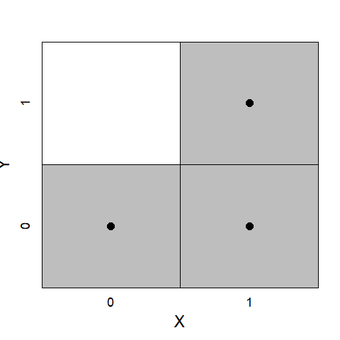
Figure 4.21: Necessity analysis by dichotomous NCA and crist set QCA.
For fuzzy set membership scores the necessity analyses of fsQCA and NCA differ. In fsQCA a diagonal is drawn in the \(XY\) scatter plot (Figure 4.22A) with data from Rohlfing & Schneider (2013); see also Vis & Dul (2018)). For necessity, there can be no cases above the diagonal. Necessity consistency is a measure of the extent to which cases are not above the diagonal, which can range from 0 to 1. When some cases are present in the ‘empty’ zone above the diagonal, fsQCA considers these cases as ‘deviant cases’. FsQCA accepts some deviant cases as long as the necessity consistency level, which is computed from the total vertical distances of the deviant cases to the diagonal, is not smaller than a certain threshold, usually 0.9. The necessity consistency is large enough, fsQCA makes a qualitative (‘in kind’) statement about the necessity of \(X\) for \(Y\): ‘\(X\) is necessary for \(Y\)’, e.g., the presence of \(X\) (membership score > 0.5) is necessary for the presence of \(Y\) (membership score > 0.5).
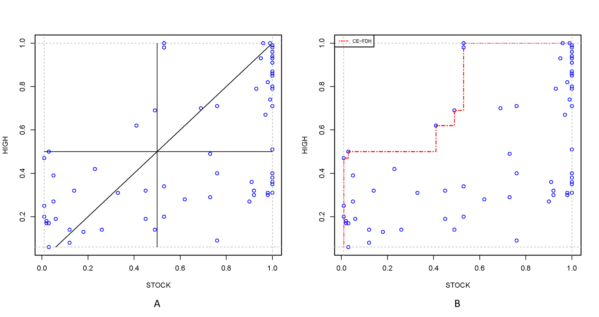
Figure 4.22: Comparison of necessity analysis with fsQCA’s (A) and with NCA (B).
4.7.2 The differences between NCA and QCA
The major differences between NCA and QCA are summarized in Figure 4.23 (see also Dul (2016a) and Vis & Dul (2018)) and discussed below.
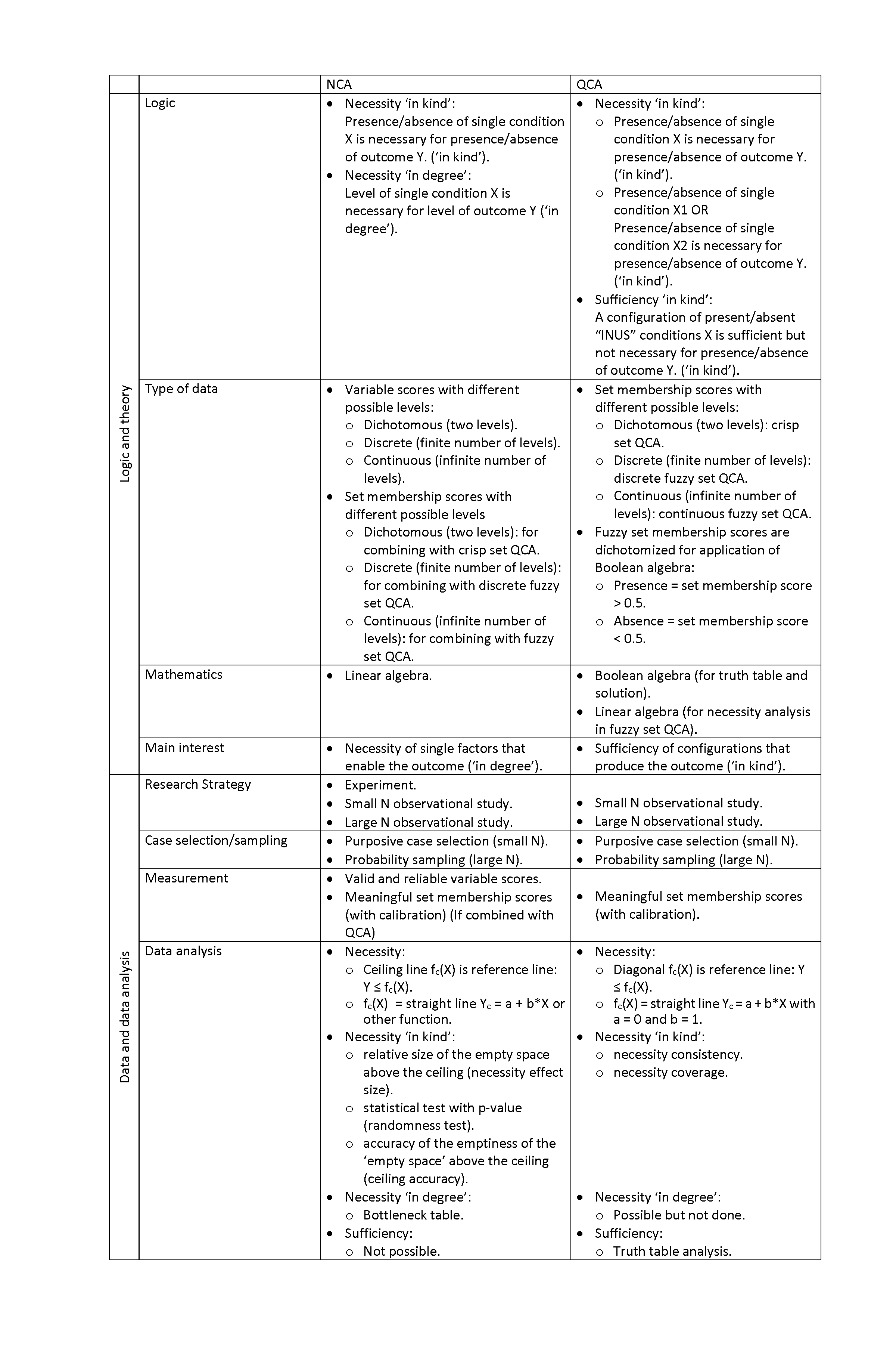
Figure 4.23: Comparison of NCA and QCA.
4.7.2.1 Logic and theory
NCA and QCA are only the same in a very specific situation of ‘in kind’ necessity: A single \(X\) is necessary for \(Y\), and \(X\) and \(Y\) are dichotomous set membership scores (0 and 1). Then the analyses of NCA and QCA are exactly the same. However, NCA normally uses variable scores, but can also set membership scores when NCA is applied in combination with QCA (see below). In addition to the ‘in kind’ necessity that both methods share, NCA also formulates ‘in degree’ necessity. QCA also formulates ‘in kind’ necessity of ‘OR’ combinations of conditions, as well as ‘in kind’ sufficiency of configurations of conditions. The main interest of NCA is the necessity ‘in degree’ of single factors that enable the outcome, whereas the main interest of QCA is the sufficiency ‘in kind’ of (alternative) configurations of conditions.
4.7.2.2 Data and data analysis
Regarding research strategy most NCA studies are observational studies (both small N and large N), although also experiments are possible. Most QCA studies are small N observational studies, although increasingly also large N studies are employed with QCA, in particular in the business and management area. The experimental research strategy is rare (if not absent) in QCA. Regarding case selection/sampling purposive sampling is the main case selection strategy in QCA. It is also possible in small N NCA studies. For large N studies sampling strategies such as those used in regression analysis (preferably probability sampling) are used both in NCA and QCA. Regarding measurement, NCA uses valid and reliable variable scores unless it is used in combination with QCA, in which case NCA uses calibrated set membership scores. QCA uses calibrated set membership scores and cannot use variable scores. In QCA data with variable scores may be used as input for the ‘calibration’ process to transform variable scores into set membership scores. Regarding data analysis in fsQCA a necessary condition is assumed to exist if the area above the diagonal reference line in an \(XY\) scatter plot is virtually empty (see Figure 4.22 A). In contrast, NCA uses the ceiling line as the reference line (see Figure 4.22 B) for evaluating the necessity of \(X\) for \(Y\) (with possibly some cases above the ceiling line; accuracy below 100%). In situations where fsQCA observes ‘deviant cases’, NCA includes these cases in the analysis by ‘moving’ the reference line from the diagonal position to the boundary between the zone with cases and the zone without cases. (Note that moving the QCA’s diagonal parallel upward to address inaccuracy has been suggested by Ragin, 2000 (p. 225, Figure 8.4), but this was not followed up by other QCA researchers). NCA considers cases around the ceiling line (and usually above the diagonal) as ‘best practice’ cases rather than ‘deviant’ cases. These cases are able to reach a high level of outcome (e.g., an output that is desired) for a relatively low level of condition (e.g., an input that requires effort). For deciding about necessity, NCA evaluates the size of the ‘empty’ zone as a fraction of the total zone (empty plus full zone), which ratio is called the necessity effect size. If the effect size is greater than zero (an empty zone is present), and if according to NCA’s statistical test this is unlikely a random result of unrelated \(X\) and \(Y\), NCA identifies a necessary condition ‘in kind’ that can be formulated as: ‘\(X\) is necessary for \(Y\)’, indicating that for at least a part of the range of \(X\) and the range of \(Y\) a certain level of \(X\) is necessary for a certain level of Y. Additionally, NCA can quantitatively formulate necessary condition ‘in degree’ by using the ceiling line: ‘level \(X_c\) of \(X\) is necessary for level \(Y_c\) of \(Y\)’. The ceiling line represents all combinations \(X\) and \(Y\) where \(X\) is necessary for \(Y\). Although also fsQCA’s diagonal reference line allows for making quantitative necessary conditions statements, e.g., \(X\) > 0.3 is necessary for \(Y\) = 0.3, fsQCA does not make such statements. When the ceiling line coincides with the diagonal (corresponding to the situation that fsQCA considers) the statement ‘\(X\) is necessary for \(Y\)’ applies to all \(X\)-levels [0,1] and all \(Y\)-levels [0,1] and the results of the qualitative necessity analysis of fsQCA and NCA are the same. When the ceiling line is positioned above the diagonal ‘\(X\) is necessary for \(Y\)’ only applies to a specific range of \(X\) and a specific range of \(Y\). Outside these ranges \(X\) is not necessary for \(Y\) (‘necessity inefficiency’). Then the results of the qualitative necessity analysis of fsQCA and NCA can be different. Normally, NCA identifies more necessary conditions than fsQCA, mostly because the diagonal is used as reference line. In the example of Figure 4.22, NCA identifies that \(X\) is necessary for \(Y\) because there is an empty zone above the ceiling line. However, fsQCA would conclude that \(X\) is not necessary for \(Y\), because the necessity consistency level is below 0.9. FsQCA’s necessity analysis can be considered as a special case of NCA: an NCA analysis with discrete or continuous fuzzy set membership scores for \(X\) and \(Y\), a ceiling line that is diagonal, an allowance of a specific number of cases in the empty zone given by the necessity consistency threshold, and the formulation of a qualitative ‘in kind’ necessity statement.
4.7.3 Recommendation for combining NCA and QCA
Although in most NCA applications variable scores are used for quantifying condition \(X\) and outcome \(Y\), NCA can also employ set membership scores for the conditions and the outcome, allowing to combine NCA and QCA. The other way around is not possible: combining QCA to a regular NCA with variable scores is not possible because QCA is a set theoretic approach that does not use variable scores. How can NCA with membership scores complement QCA? For answering this question first another question should be raised: how does QCA integrate an identified necessary condition in kind with the results of the sufficiency analysis: the identified sufficient configurations. By definition the necessary condition must be part of all sufficient configurations, otherwise this configuration cannot produce the outcome. However, within the QCA community five different views exist about how to integrate necessary conditions in sufficiency solution. In the first view only sufficient configurations that include the necessary conditions are considered as a result. Hence, all selected configurations have the necessary condition. In the second view the truth table analysis to find the sufficient configurations are done without the necessary conditions and afterwards the necessary conditions are added to the configuration. This also ensures that all configurations have the necessary conditions. In the third view configurations that do not include the necessary condition are excluded from the truth table before this table is further analysed to find the sufficient configurations. This ‘ESA’ approach (Schneider & Wagemann, 2012) also ensures that all configurations have the necessary conditions. In the fourth view sufficient configurations are analysed without worrying about necessary conditions. Afterwards, the necessary conditions are discussed separately. In the fifth view a separate necessity analysis is not done, or necessity is ignored. All views have been employed in QCA; hence no consensus exists yet. And additional complexity of integrating necessity with sufficient configuration is that NCA produces necessary conditions in degree, rather than QCA’s necessary condition and sufficient configurations in kind. The conditions that are part of the sufficient configurations can only be absent or present. Given these complexities, I suggest, a combination of the second and the fourth view:
Perform the NCA analysis ‘in degree’ before QCA’s sufficiency analysis.
Integrate a part of the results of NCA’s necessity analysis into QCA’s sufficient configurations, namely the conditions (‘in degree’) that are necessary for outcome > 0.5. (use the NEST Tool: the NCA-Extended Solution Table, which adds a column to QCA’s solution table based on NCA results)
Discuss the full results of NCA’s necessity analysis afterwards.
In particular it could be discussed that specific levels of necessary membership scores found by NCA must be present in each sufficient configuration found by QCA. If that membership in degree is not in place, the configuration will not produce the outcome.
4.7.4 Examples
I discuss two examples of integrating NCA in QCA according to this recommendation. The first example is a study by Emmenegger (2011) about the effects of six conditions: S = state-society relationships, C = non-market coordination, L = strength labour movement, R = denomination, P = strength religious parties and V = veto points on JSR = job security regulation in Western European countries. He performed an fsQCA analysis with a necessity analysis and a sufficiency analysis. His necessity analysis showed that no condition was necessary for job security regulation (necessity consistency of each condition was < 0.9).
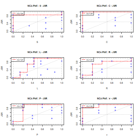
Figure 4.24: Example of a necessity analysis with NCA (Data from Emmenegger (2011).
However, the NCA analysis in degree with the six conditions and using the CE-FDH ceiling line (Figure 4.24) shows the following effect sizes and corresponding p values (Figure 4.25).

Figure 4.25: NCA necessity analysis. d = effect size; p = p value.
A condition could be considered necessary when the effect size has a small p value (e.g., p < 0.05). Hence, the NCA analysis shows that certain strength of labour movement (L), a certain level of denomination (R), and a certain strength of religious parties (P) are necessary for high levels of job security regulation (JSR). From Figure 4.24 it can be observed that the following conditions are necessary for JSR > 0.5:
L > 0.29 is necessary for JSR > 0.5 (presence of JSR)
R > 0.20 is necessary for JSR > 0.5 (presence of JSR)
P > 0.20 is necessary for JSR > 0.5 (presence of JSR)
Although in QCA’s binary logic these small necessary membership scores of L, R, P (all < 0.5) would be framed as ‘absence’ of the condition, in NCA these membership scores are considered small, yet must be present for having the outcome. Thus, according to NCA the low level of membership scores must be present, otherwise the sufficient configurations identified by QCA will not produce the outcome. Emmenegger (2010) identified four possible sufficient configurations for the outcome JSR:
S*R*~V (presence of S AND presence of R AND absence of V)
S*L*R*P (presence of S AND presence of L AND presence of R AND presence of P)
S*C*R*P (presence of S AND presence of C AND presence of R AND presence of P)
C*L*P*~V (presence of C AND presence of L AND presence of P AND absence of V)
This combination of solutions can be expressed by the following logical expression: S*R*~V + S*L*R*P + S*C*R*P + C*L*P*~V → JSR The presence of a condition and the outcome means that the membership score is > 0.5. The absence of a condition means that the membership score is < 0.5. A common way to summarize the results is shown in Figure 4.26.

Figure 4.26: QCA sufficiency solutions (sufficient configurations).
The NCA necessity results can be combined with the QCA sufficiency results as shown in Figure 4.27.
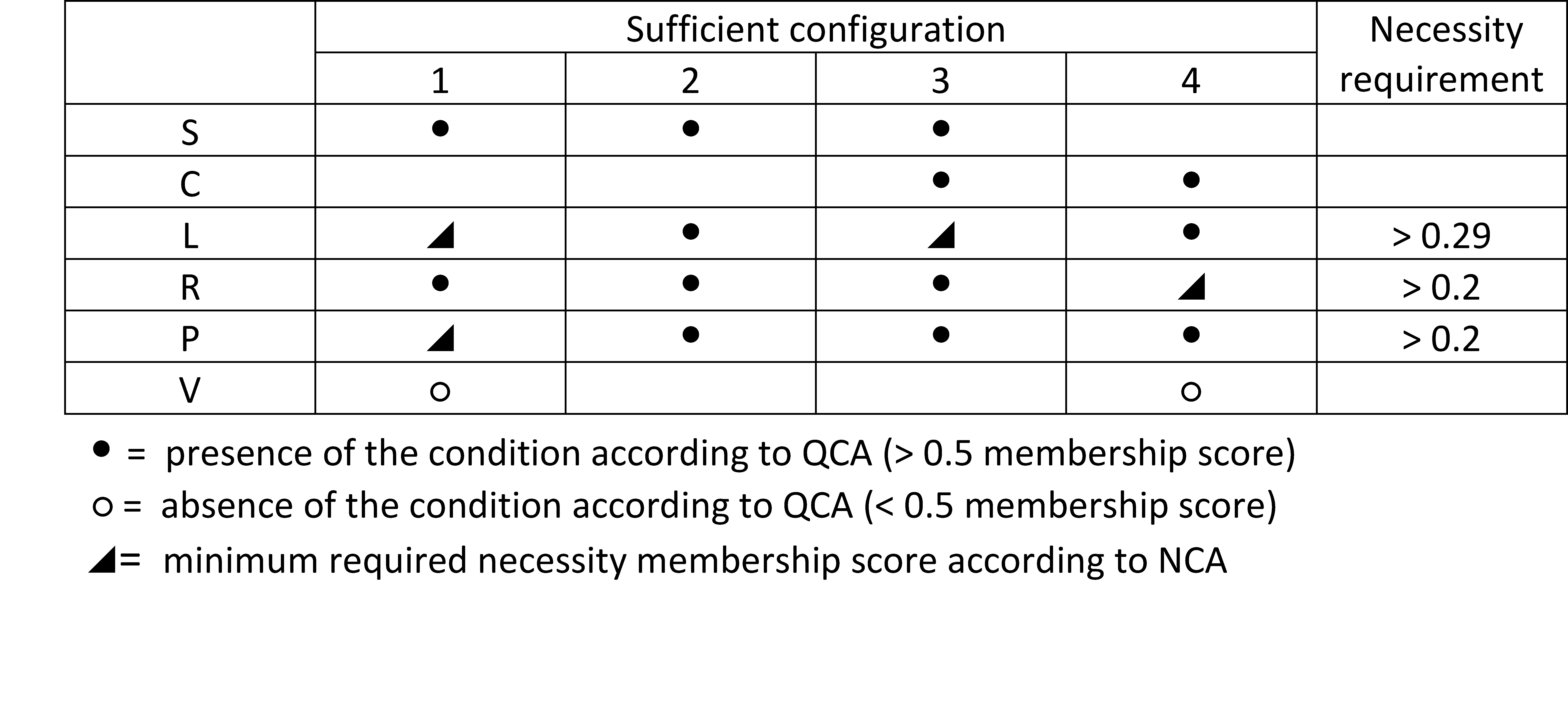
Figure 4.27: NEST tool for combining QCA sufficiency results with NCA necessity results. NEST = NCA-Extended Solution Table. The extension consist of adding the symbol ◢ when the necessary condition in degree is missing in the sufficiency solution, and adding the column ‘Necessity requirement’ with the required level of the necessary condition.
Figure 4.27 presents the NEST tool, which is the NCA-Extended Solution Table. NEST signifies if a necessary condition ‘in degree’ is missing in the configuration. If so, the triangle symbol (◢) is added to the sufficient QCA configuration to ensure that the minimum required necessity membership score (according to NCA) is fulfilled such that the solution can produce the outcome. The triangle symbol ◢ for necessity ‘in degree’ differs from the square symbol ■ proposed by Greckhamer (2016), and the diamond symbol \(\blacklozenge\) used by Holtrop et al. (2024), which both indicate the presence of a necessary condition ‘in kind’ according to QCA’s necessity analysis. An additional column ‘Necessity requirement’ is added to ensure that the minimum required necessity membership score (according to NCA) is fulfilled such that the solution can produce the outcome. Note that a condition with 0.29 membership score is not interpreted in a binary ‘in kind’ way as the absence of the condition (although the score is < 0.5), but as an ‘in degree’ interpretation where to condition is ‘somewhat’ (0.29) present, like a pinch of salt is necessary for a tasty cake.
The NCA results that the presence of L > 0.29 is necessary for JSR > 0.5 is already achieved in the QCA sufficient configurations 2 and 4, but not in configurations 1 and 3. In these latter configurations the requirement L > 0.29 is added to the configuration (◢). Similarly, R > 0.20 is added to configuration 4, and P > 0.20 is added to configuration 1. Without adding these requirements to the configuration, the configuration cannot produce the outcome. Only configuration 2 includes all three necessary conditions according to NCA, without a need for adding them. If the results of NCA would be ignored and the QCA of configurations 1, 3 and 4 would not produce the outcome (or only by chance if the required minimum levels of the ignored NCA necessary conditions would be present by chance). Additionally, the NCA results can show what levels of the condition would be necessary for a higher level of the outcome than a membership score > 0.5. This can be observed in Figure 3. For example, for a membership score of JSR of 0.9, it is necessary to have membership scores of S = 1, L > 0.45, R = 1, P > 0.2, and ~V > 0.35. I therefore recommend presenting the NCA necessity results together with the QCA sufficient configurations results as in Figure 4.27, and additionally to discuss the full results of NCA for deeper understanding of the sufficient configurations.
The second example is from a study of Skarmeas et al. (2014) that I discuss in my book (Dul, 2020, pp. 77-83). This study is about the effect of four organizational motives (Egoistic-driven motives, absence of Value-driven motives, Strategy-driven motives, Stakeholder-driven motives) on customer scepticism about an organization’s Corporate Social Responsibility (CSR) initiative. The results of NCA’s necessity analysis with raw scores, and with calibrated set membership scores are shown in Figure 4.28 and Figure 4.29, respectively.

Figure 4.28: NCA necessity analysis with raw scores.

Figure 4.29: NCA necessity analysis with calibrated cores.
NCA with raw variable scores shows that Absence of Value-driven motives and Strategy-driven motives could be considered are necessary for Scepticism given the medium effect sizes and the small p values (p < 0.05). Also, the NCA with calibrated set membership scores shows that these two conditions have low p values; however, their effect sizes are small (0.04 and 0.02, respectively). This means that these necessary conditions may be statistically significant but may not be practically significant: nearly all cases reached the required level of necessity. Also, Egoistic-driven motives are statistically, but not practically significant. NCA with raw variable scores (the conventional NCA approach) can be used in combination with regression analysis, as regression analysis uses raw variable scores. NCA with calibrated set scores (set membership scores) can be used in combination with QCA, because QCA uses calibrated set membership scores.
Figure 4.30 shows the two sufficient configurations according the QCA analysis of Skarmeas et al. (2014). (2014).

Figure 4.30: Sufficient configurations (QCA) and necessity requirements (NCA) of the study by Skarmeas et al., 2014.
In each configuration the necessity of Egoistic-driven motives and the Absence of Valuedriven motives are ensured in the configuration. However, the necessity of Strategy-driven motives is not ensured in Sufficient configuration 1. Therefore, the minimum required level of Stakeholder-driven motives according to NCA (0.01) is added to ensure that the configuration is able to produce the outcome. However, the practical meaning of this addition is very limited because the necessity effect size is small. It is added here for illustration of our recommendation.
4.7.5 Logical misinterpretations when combining NCA and QCA
When NCA is combined with QCA sometimes a logical misinterpretation is made about the role of necessary conditions in sufficient configurations. Although a factor that is a necessary condition for the outcome must be part of each sufficient configuration, the opposite is not true: a factor that is part of the sufficient configuration must not automatically be a necessary condition for the outcome. The latter misinterpretation has been introduced in the tourism and hospitality field (Dul, 2022) and can be found for example in studyies by Farmaki et al. (2022), Pappas & Farmaki (2022), Pappas & Glyptou (2021b), Pappas & Glyptou (2021a), Pappas (2021), and Farmaki & Pappas (2022). The misinterpretation was also exported to other fields (e.g., Mostafiz et al., 2023).
This misinterpretation may be caused by mixing necessary conditions for the outcome (as analysed with NCA) with necessary parts of a sufficient configuration (INUS conditions). An INUS condition is an Insufficient but Necessary part of an Unnecessary but Sufficient configuration. INUS conditions are the necessary elements of a configuration to make that configuration sufficient. NCA captures necessary conditions for the outcome, not INUS conditions, see also Dul, Vis, et al. (2021).
4.8 Causal inference
Applications of NCA often use cross-sectional research designs. In order to make a causal interpretation of findings from a cross-sectional study, several requirements need to be met. Cross-sectional studies observe cases at a single point in time without manipulating variables. This contrasts with experimental studies where potential causes are manipulated and effects are observed, which allows a direct causal interpretation. Cross-sectional studies can infer causality only indirectly if certain criteria are fulfilled. These criteria include: relevant association, temporal sequence, theoretical plausibility, and control of confounders. Because of the way that necessity is defined, NCA findings are immune to confounding because the observed necessity relationship is not influenced by including or excluding other variables. Therefore, the three main requirements for inferring causality from an NCA cross-sectional study are (1) observing a relevant association, (2) justifying a temporal sequence, and (3) formulating a plausible theory.
In NCA the requirement for observing a relevant association between \(X\) and \(Y\) means observing that one of the corners of an \(XY\) plot is empty (rather than observing a correlation). When it is expected that the presence of \(X\) is necessary for the presence of \(Y\) the expected empty corner is in the upper left corner.
The requirement for observing a relevant association can be satisfied by having proper values of NCA’s effect size (e.g., \(d\geq0.10\)) representing practical relevance and p value (e.g., \(p\leq0.05\)) representing statistical relevance.
The requirement for justifying the temporal sequence implies that there must be evidence that \(X\) precedes \(Y\): first \(X\) then \(Y\). If \(X\) precedes \(Y\), the empty space is compatible with \(X\) being necessary for \(Y\). However, if \(Y\) precedes \(X\) the empty space is compatible with \(Y\) being sufficient for \(X\) (reverse causality). If both directions can be theoretically justified the empty space may be compatible with reciprocal (bi-directional) causality: \(X\) is necessary for \(Y\), and \(Y\) is sufficient for \(X\). The requirement for justifying a temporal sequence can be satisfied as part of the formulation of a plausible theory (see below).
The requirement for formulating a plausible theory implies that there should be a rational explanation how \(X\) is a necessary cause for \(Y\). This means that the expected causal direction and the causal mechanism are explained theoretically. This requirement is usually satisfied by formulating a hypothesis for example “the presence of \(X\) is a necessary cause for the presence of \(Y\)”, while specifying and justifying the temporal direction, and explaining the mechanism why this relationship exists. Explaining the necessity mechanism can be done by explaining the enabling mechanism why cases with the outcome must have the condition, or by explaining the constraining mechanism why cases without the condition cannot have the outcome and why the absence of this condition is not compensible.
If the above requirements are not convincingly met, an alternative research design may be selected to infer causality. In order of increasing confidence, this can be the time-lagged study design in which \(X\) is measured first followed by \(Y\), the longitudinal study design in which \(X\) and \(Y\) are measured in multiple points in time, and the experimental study design in which \(X\) is manipulated and the effect on \(Y\) is observed.
In practical applications of NCA each of the following requirements need to be fulfilled to interpret an empty space as a necessary causal condition:
- Theoretical support that \(X\) is a necessary cause for \(Y\) (causal direction, mechanism).
- The corresponding empty space is relevant (e.g., \(d \geq 0.10\)).
- The p value of the empty space is small (e.g., p \(\leq 0.05\)).
If one of the conditions is not met, it cannot be concluded that there is empirical evidence for necessity causality.
4.9 Meta-analysis
Given the growth of NCA publications (see Figure 0.1 and Table 0.1), it can become a realistic option to conduct a meta-analysis of NCA studies for a specific topic. The general aim of a meta-analysis is to systematically combine results from multiple independent studies that address the same research question. A common goal is to estimate an overall effect size across studies by combining results from different samples. This gives an estimate of the ‘true’ effect size in an underlying population from which the samples are assumed to be drawn. This is done, by estimating an overall mean effect size using weighting of the effect sizes of the different samples (e.g., based on sample size). In other words, a weighted average is used as an estimate of the overall effect size. The assumption is made that the effect sizes can be compared (e.g., in each study the \(XY\) variables are measured on the same scale), and that there is no measurement error.
However, this approach does not apply to NCA because the sample necessity effect size is always larger than the true effect size, such that the weighted average of the sample effect sizes is not a proper representation of the true effect size. Instead, with the same assumptions as in a regular meta-analysis (no measurement error, comparable effect sizes), and an additional assumption that the scopes of the separate studies are the same (empirically or by setting the same theoretical scope for each study), the minimum of the sample effect sizes might be the best representation of the true effect size. Alternatively, and probably even more convincing, all samples could be combined into one master sample (as they are assumed coming from the same population) and then the effect size of the combined sample could be the estimation of the true effect size. Such meta-analysis is called an “individual participant meta-analysis” (IPD meta-analysis) and assumes that raw data are available. If it cannot be assumed that the samples are from the same (underlying) population, then differences in sample effect sizes could be explained by the different characteristics of the population. If absence of measurement error cannot be assumed, then an NCA outlier-analysis may possibly find cases with measurement error that could have partly caused sample effect size differences (and could be deleted).
References
See for example the advise “While a non-significant effect provides evidence that a total effect is zero in the population, researchers should retain the corresponding construct in the IPMA since this outcome may also represent a valuable finding (e.g., a company invests into the performance of a construct that has no effect), which also can change with different data, for instance, in alternative contexts of the analysis” (Ringle & Sarstedt, 2016, p. 1872), and the practice of the example in Hauff et al. (2024) that includes non-significant total effects in CIPMA↩︎
This aligns with NCA’s recommendation that the absence of any of the three critical requirements for support for necessity falsifies the necessary condition claim: the absence of theoretical support (no necessity hypothesis), the absence of a practically relevant effect size (e.g., \(d < 0.10\)), and a statistically non-significant necessity effect size (e.g., \(p > 0.05\)).↩︎