Chapter 6 NCA’s statistics
[Acknowledgement: Roelof Kuik contributed to this Chapter]
The central idea underlying NCA is that of an area in the \(XY\) plane exists that does not hold data. This empty space is defined by the ceiling line and the scope (bounds on the variables). No assumptions beyond such empty space are being made. So, the theory does not require specification of probability distributions or data generation processes for the area that can hold data, the feasible area (area under the ceiling). Rather than turning to probability theory, NCA bases its analysis on the empty spaces and uses geometry (relations between data points in terms of distances and areas) for developing its notions of strength of estimated ceilings (through calculation of an effect size), and cardinality (number of elements in a set) for measures of fit (ceiling accuracy). Still, NCA is not at odds with assumptions from probability theory or statistics. Extending NCA with such assumptions allows the use of statistical techniques into the analysis.
This chapter discusses two statistical techniques that can be used in the context of NCA. First, NCA’s statistical significance test is a null hypothesis test that evaluates if NCA’s observed effect size could be compatible with effect sizes produced by two unrelated variables. The test rejects the null hypothesis when there is a low probability that the observed effect is a random result of unrelated variables (e.g., p < 0.05). NCA’s statistical test is one of the three parts of NCA. The other parts are the use of necessity logic for formulating the causal assumptions (hypotheses), and the data analysis to calculate the NCA effect size. Second, Monte Carlo simulations with NCA may be performed. Such statistical simulations requires an assumption about the probability distribution of the data in the feasible area. This chapter shows three examples of simulations: estimation of the power of NCA’s statistical test, evaluation of the quality of effect size and ceiling line estimations, and demonstration that necessity can produce correlation.
6.1 NCA’s statistical expression
Based on NCA’s mathematical backgrounds (see Chapter 5), NCA employs a bivariate statistical data analysis for each condition separately (multiple bivariate analysis). The statistical model of NCA can be expressed by an equality equation as
\[\begin{equation} \tag{6.1}y = f(x_i) - \epsilon_{x_i} \end{equation}\]
Here the function \(f(x_i)\) represents the border line of the i-th condition in the \(X_iY\) plane and \(\epsilon_{x_i}\) is a random variable that takes on non-negative values only (when the border line is a ceiling line, i.e., when the upper left or upper right corner of the \(XY\) plot are empty) or a non-positive value only (when the border line is a floor line, i.e. when the lower left or lower right corner of the \(XY\) plot are empty). In the remainder of this Chapter it is assumed that the empty space is in the upper left corner and the error term is non-negative. The NCA model assumes that \(X\) and \(Y\) are bounded (have minimum and maximum values) and that there are no errors of measurement in variables \(X\) and \(Y\). The NCA model does not make strong assumptions about the error term (e.g., no assumption about the type of distribution, the mean value, or the variance). The NCA model differs from a regression model. The regression model is expressed as
\[\begin{equation} \tag{6.2}y = f(x) + \epsilon_x \end{equation}\]
Here the function \(f(x)\) has additive terms consisting of (combinations of) \(X\)’s with coefficients. The regression model assumes that \(X\) and \(Y\) are unbounded variables (can have values between minus and plus infinity) and that there are no errors of measurement in variables \(X\) and \(Y\). The regression model makes several strong assumptions about the error term. For example, it is assumed that \(\epsilon_x\) is independent of \(X\), its average value is zero, and its variance does not depend on \(X\). Additionally, it is often assumed that the errors are normally distributed. Therefore, \(f(x)\) describes the average effect of \(X\) on \(Y\) such that conventional regression techniques are not appropriate for modeling necessity relationships.
NCA’s statistical approach is a ‘semi-parametric’ approach, that only specifies particular features of the distribution (in NCA: the ceiling line, bounded variables within a scope) but not the distribution itself (Greene, 2012, p. 482). Thus, NCA does not require making assumptions about the distributions of \(X\), \(Y\) and \(\epsilon_x\). NCA only specifies a part of the Data Generation Process (DGP): the ceiling function of bounded variables within the scope. NCA does not specify how the data below the ceiling are generated, thus no further specification of \(\epsilon_x\) is needed. This is inherent to NCA’s goal of analyzing necessary but not sufficient conditions: a certain level of \(X\) is required for having a certain level of \(Y\) but it does not automatically produce that level of \(Y\): NCA does not predict \(Y\).
6.2 NCA’s statistical test
NCA’s statistical test is a null hypothesis test that estimates a p value for the effect size using a permutation approach (Dul, 2020; Dul, Van der Laan, et al., 2020)4. Mathematical proofs and simulations have shown (Dul, Van der Laan, et al., 2020) that the estimated p value of NCA’ statistical test is valid. Indeed, the validity of the permutation test on which NCA is based is a theorem (Hoeffding, 1952; Kennedy, 1995; Lehmann et al., 2005). NCA’s statistical test can be classified as a permutation and randomization test in the terminology of Lehmann et al. (2005). The justification of the test rests on the so-called Randomization Hypothesis being true. The Randomization Hypothesis states (see Lehmann et al., 2005, p. 633):
Under the null hypothesis, the distribution of the data \(X\) is invariant under the transformation \(g\), that is, for every transformation \(g\) in \(G\), \(gX\) and \(X\) have the same distribution whenever \(X\) has distribution \(P\) in H0.
In this context \(G\) is the group of permutations of \(n\) elements. The transformation of the sample data \(S\) under a permutation \(g\) in \(G\) is here \(S \mapsto gS\) and the Randomization Hypothesis is that \(S\) and \(gS\) have the same distribution when \(S\) has been sampled from a distribution in NCA’s H0 (variables are independent). In other words, under the Randomization Hypothesis, repeated sampling of \(S\), with each time making \(gS\), the distributions of \(S\) and \(gS\) should be the same. For NCA’s statistical test this condition is satisfied.
NCA’s statistical test is a part of an entire NCA method consisting of (1) formulating necessity theory, (2) calculating necessity effect size (relative size of empty space in \(XY\) plot) and (3) performing a statistical test. Within this context the test has a specific purpose of testing the randomness of the empty space when \(X\) and \(Y\) are unrelated. Therefore, a test result of a large p value (e.g., p > 0.05) means that the empty space is compatible with randomness of unrelated variables. A test result of a small p value (e.g., p < 0.05) means that the empty space is not compatible with randomness of unrelated variables. However, falsifying H0 does not mean that a specific H1 is accepted. The goal of a null-hypothesis test is to test the null (H0) not a specific alternative (H1). The p value is only defined when the null is true. However, the p value is not defined when a specific H1 is true. Therefore, the p value is not informative about which H1 applies. This is a general characteristic of the p value that is often misunderstood. “A widespread misconception … is that rejecting H0 allows for accepting a specific H1. This is what most practicing researchers do in practice when they reject H0 and argue for their specific H1 in turn” (Szucs & Ioannidis, 2017, p. p8).
NCA’s statistical test is only a part of the entire NCA method. With a high p value, the tests accepts the null, and rejects any H1 (including necessity). With a low p value the test rejects the null, but does not accept any specific H1, thus also not necessity. It depends on the results of the entire NCA method (including theory and effect size) and of the researcher’s judgment whether or not necessity is plausible, considering all evidence. Therefore, NCA’s statistical test result of a low p value is a ‘necessary but not sufficient condition’ for concluding that an empty space be considered to be caused by necessity (Dul, Van der Laan, et al., 2020). The test protects the researcher from making a false positive conclusion, namely that necessity is supported when the empty space is likely a random result of two unrelated variables.
6.3 Simulations with NCA
6.3.1 Requirements for simulations with NCA
Although NCA does not specify the full DGP, for conduction simulations the full DGP needs to be specified by the researcher for being able to do such simulation. This means that the researcher must make not only a choice for the ‘true’ ceiling line in the population (\(f(x_i)\)), but also for the distribution of the error term (\(\epsilon_x\)) in equation (6.1). For making this choice two fundamental assumptions of NCA must be met:
A sharp border exist between an area with and without observations defined by the ceiling line (to represent necessity theory: no \(Y\) without \(X\)).
\(X\) and \(Y\) are bounded.
The ceiling line can be linear or non-linear. The distribution of \(X\) and \(Y\) must be bounded. Valid examples of commonly used bounded distributions are the uniform distribution and the truncated normal distribution. The NCA software in R from version 4.0.0 includes the function nca_random that can be used in NCA simulations. Input arguments are the number of observations (N), the intercept of the ceiling line, the slope of the ceiling line, and the type of distribution under the ceiling (uniform-based or truncated normal-based).
library(NCA)
#generate random data
set.seed(123)
data <- nca_random(100, # sample size
                   0.2, # ceiling intercept
                   1,   # ceiling slope
                   distribution.x = "uniform", # distribution under the ceiling
                   distribution.y = "uniform"  # distribution under the ceiling
                   )
model <- nca_analysis(data, "X", "Y", ceilings = "c_lp")
nca_output(model)
model$summaries$X$params[10] # estimated intercept (true intercept = 0.2)
model$summaries$X$params[9] # estimated intercept (true slope = 1.0)
The nca_random function produces a bivariate distribution of \(X\) and \(Y\) of points below the ceiling line within the scope [0,1] by first assuming distributions for \(X\) and \(Y\) separately (uniform or truncated normal) and then combine them into one bivariate distribution by removing points above the ceiling line. Figure 6.1 shows two typical random samples of n = 100, one drawn from the uniform-based bivariate distribution (A), and one from the truncated normal-based bivariate distribution (B). In this example, the true ceiling line in the populations has a slope of 1 and an intercept of 0.367544468, resulting in a true necessity effect size of 0.2.
Figure 6.1: Typical sample (n = 100) from a population with true straight ceiling line and effect size = 0.2 with a uniform-based distribution (A) and a truncated normal-based distribution (B).
Note that a necessity relationship cannot be simulated with unbounded distributions such as the normal distribution. With unbounded variables a necessity effect cannot exist in the population. For example, NCA’s necessity effect size for bivariate normal variables is zero in the population. A possible empty space in a sample is not the result of a necessity effect in the population but a result of finite sampling. Thus, a sample empty space has no necessity meaning when the population distribution of the variables is unbounded. With unbounded distributions, a finite sample always leads to a finite (empirical) scope (box) that allows the computation of an ‘effect size’. But, such quantity is not related to necessity as defined in NCA. Producing a number out of a sample is an estimate of some property in the population, but the question is what estimand/property of the population distribution it corresponds to. With population data assumed being generated from an unbounded distribution, empirical scopes would grow beyond any bound with growing size of the sample.
6.3.2 Simulations for estimating the power of NCA’s statistical test
“The power of a test to detect a correct alternative hypothesis is the pre-study probability that the test will reject the test hypothesis (the probability that \(p\) will not exceed a pre-specified cut-off such as 0.05)” (Greenland et al., 2016, p. 345). The higher the power of the test, the more sensitive the test is for identifying necessity if it exists. Knowledge about the power of NCA’s statistical test is useful for planning an NCA study. It can help to establish the minimum required sample size for being able to detect with high probability (e.g., 0.8) an existing necessity effect size that is considered relevant (e.g., 0.10). Note that a post-hoc power calculation as part of the data analysis of a specific study does not make sense (Christogiannis et al., 2022; Lenth, 2001; e.g., Zhang et al., 2019). In a specific study, power does not add new information to the p value. Because power is a pre-study probability, a study with low power (e.g., with a small sample size) can still produce a small p value and conclude that an necessary condition exists, although the probability of identifying this necessity effect is less than with a high powered study (e.g., with a large sample size).
Statistical power increases when effect size and sample size increase. For a given expected necessity effect size in the population, the probability of not rejecting the null hypothesis when necessity is true can be reduced by increasing the sample size.
The power of NCA’s statistical test can be evaluated by using the nca_power function which is available from NCA software version 4.0.0.in R. The simulation presented here includes five population effect sizes ranging from 0.10 (small) to 0.5 (large) (Figure 6.2). The population effect size is the result of a straight population ceiling line with slope = 1 and an intercept that corresponds to the given population effect size.
Figure 6.2: Five ceiling lines (slope = 1) with corresponding effect sizes of of 0.1, 0.2, 0.3, 0.4, and 0.5.
For the simulation a large number of samples (500) of a given sample size are randomly drawn from the bivariate population distribution. This is done for 2 x 5 x 11 = 110 situations: two bivariate distributions (uniform-based or truncnormal-based), five effect sizes (0.1, 0.2, 0.3, 0.4, 0.5), and 11 sample sizes (5, 10, 20, 30, 40, 50, 100, 200, 500, 1000, 5000). In each situation, NCA’s p value is estimated for all 500 samples. The power is calculated as the proportion of samples with estimated p value less than or equal to the selected threshold level of 0.05. This means that if, for example, 400 out of 500 samples have p \(\le0.05\), the power of the test in that situation is 0.8. A power value of 0.8 is a commonly used benchmark for a high powered study. For an acceptable computation time the number of permutations to estimate NCA’s p value for a given sample is limited to 200, and the number of resamples is set to 500; more accurate power estimations are possible with more permutations and more resamples.
The details of the simulation (which may take several hours) are as follows:
library(NCA)
library(ggplot2)
# simulation parameters
rep = 500  #number of datasets (repetitions, iterations)
test.rep = 200  #number of permutations
p.Threshold = 0.05  #pvalue threshold alpha
distribution = c("uniform", "normal")
ns <- c(5, 10, 20, 30, 40, 50, 100, 200, 500, 1000, 5000)  #sample sizes
true.effect <- c(0.1, 0.2, 0.3, 0.4, 0.5)  #true effect sizes
true.slope <- 1  #rep(1,length(true.effect)) #true slope
results <- matrix(nrow = 0, ncol = 8)  # for storing simulation results

# simulation
set.seed(123)
for (d in distribution) {
    power <- nca_power(n = ns, effect = true.effect, slope = true.slope,
        ceiling = "ce_fdh", p = p.Threshold, distribution.x = d,
        distribution.y = d, rep = rep, test.rep = test.rep)
    results <- rbind(results, power)
}

# powerplot: x axis is sample size; y axis is power
for (d in distribution) {
    dfs <- subset(results, results$distr.x == d & results$distr.y ==
        d)
    dfs$ES <- as.factor(dfs$ES)
    dfs$n <- factor(dfs$n, levels = ns)
    dfs$power <- as.numeric(dfs$power)
    p <- ggplot(dfs, aes(x = n, y = power, group = ES, color = ES)) +
        geom_line() + ylim(0, 1) + geom_hline(aes(yintercept = 0.8),
        linetype = "dashed") + theme_minimal() + labs(color = "Effect size") +
        labs(color = "Effect size") + labs(x = "Sample size",
        y = "Power")
    print(p)
}
The relationship between sample size and power for different population necessity effect sizes is shown in Figure 6.3 for the uniform distribution and in Figure 6.4 for the truncated normal distribution. The figures show that when the effect size to be detected is large, the power increases rapidly with increasing sample size. A large necessity effect of about 0.5 can be detected nearly always (power ~ 1.0) with a sample size of about 30. However, to obtain a high power of 0.8 for a small effect size of about 0.1, the sample size needs to be doubled with a uniform distribution (about 60) and be more than 10 times larger (about 300) with a truncated normal distribution. In general, the minimum required effect size for detecting a necessary condition is larger for a truncated normal distribution than for a uniform distribution. Additional simulations indicate that sample sizes must be larger when the the density of observations near the ceiling is smaller, in particular when there are few cases in the upper right or lower left corners under the ceiling. Also larger minimum samples sizes are usually needed when the ceiling line is more horizontal and to a lesser extend when it is more vertical. On the other hand, when sample sizes are large even very small effect sizes (e.g., 0.05) can be detected. Note that a high powered study only increases the probability of detecting a necessity effect when it exists. Low powered studies (e.g., with a small sample size) can still detect necessity (\(p \leq 0.05\)), but have a higher risk of making a false negative conclusion: concluding that necessity does not exist, whereas it actually exists. Note also that small N studies can easily falsify a dichotomous necessary condition where \(X\) and \(Y\) can have only two values, when the necessary condition does not exist in the population (see section 3.3.1).
Figure 6.3: Power as a function of sample size andeffect size for a uniform-based distribution.
Figure 6.4: Power as a function of sample size and effect size for a truncated normal-based distribution.
6.3.3 Simulations for evaluating a ceiling line and its effect size
When analysing sample data for statistical inference, the calculated ‘statistic’ (in NCA the ceiling line and its effect size) is an estimator of the ‘true’ parameter in the population. An estimator is considered to be a good estimator when for finite (small) samples the estimator is unbiased and efficient, and for infinite (large) samples the estimator is consistent. Unbiasedness indicates that the mean of the estimator for repeated samples corresponds to the true parameter value; efficiency indicates that the variance of the estimator for repeated samples is small compared to other estimators of the population parameter. Consistency indicates that the mean of the estimator approaches the true value of the parameter and that the variance approaches zero when the sample size increases. When the latter applies, the estimator is called asymptotically unbiased, even if the estimator is biased in finite (small) samples. An estimator is asymptotically efficient if the estimate converges relatively fast to the true population value when the sample size increases.
There are two ways to determine the unbiasdness, efficiency and consistency of estimators: analytically and by simulation. In the analytic approach the properties are mathematically derived. This is possible when certain assumptions are made. For example the OLS regression estimator of a linear relationship in the population is ‘BLUE’ (Best Linear Unbiased Estimator) when the Gauss-Markov assumptions are satisfied (the dependent variable is unbounded, homoskedasticity, error term unrelated to predictors, etc.).
In the simulation approach a Monte Carlo simulation is performed in which first the true parameters (of variables and distributions) in the population are defined, then repeated random samples are drawn from this population, and next the estimator is calculated for each sample. Finally, the sampling distribution of the estimator is determined and compared with the true parameter value in the population.
For both approaches the following ‘ideal’ situation is usually assumed: the population is infinite, the samples are drawn randomly, the distributions of the variable or estimates are known (e.g. normal distribution), and there is no measurement error. Without these assumptions the analysis and simulations get very complex.
For NCA, no analytical approach exists (yet) to determine bias, efficiency and consistency of its estimators (ceiling lines and their effect sizes) so currently NCA relies on simulations to evaluate the quality of its estimates.
For estimating the ceiling line and effect size with empirical data for \(X\) and \(Y\), two default estimation techniques are available. The first default technique is Ceiling Envelopment - Free Disposal Hull (CE-FDH), which is a local support boundary curve estimation techniques. The free disposal hull (FDH) constructs a space (the hull) encompassing the observations. The FDH is the smallest space encompassing the data points that has the free disposal property. A space is said to have the free disposal property (e.g., Simar & Wilson, 2008), if having a particular point implies that it also includes the points at the lower right of that point. The boundary of the FDH hull is a non-decreasing step function, which can serve as an estimate of the ceiling line, in particular when \(X\) or \(Y\) are discrete, or when the ceiling line is not straight.
The second default technique is Ceiling Regression - Free Disposal Hull (CR-FDH), which is a global support boundary, frontier function and curve estimation technique. The CR-FDH ceiling line is a straight trend line through upper left points of the CE-FDH line using OLS regression. Consequently, the CR-FDH ceiling line has some cases in the otherwise empty space. Therefore, in contrast to CE-FDH, the ceiling accuracy of CR-FDH is usually below 100 percent.
In addition to the two default ceiling lines, another straight line ceiling technique that is available in the NCA software is Ceiling - Linear Programming (C-LP). This estimation approach uses linear programming; a technique that optimizes a linear goal function under a number of linear constraints. When applied to NCA the technique draws a straight line through two corner points of CE-FDH such that the area under the line is minimized.
Monte Carlo simulation is used for estimating the true effect size in a population using the three types of ceiling line (CE-FDH, CR-FDH and C-LP). Variable X has a necessity relationship with Y, represented by a straight ceiling line (Y = 0.4 + X). The corresponding true effect size is 0.18.
In Monte Carlo simulation the full ‘Data Generation Process’ (DGP) needs to be specified. This means that also assumptions must be made about the distribution of the data under the ceiling line. In this simulation we assume a uniform distribution under the ceiling line, normalized for the vertical distance under the ceiling line. Additional simulations have been done with different distributions (Massu et al., 2020) but the similar results are not reported here. The simulation is done with 100 resamples per sample size. The seven sample size vary between 20 and 5000. This is repeated for each type of ceiling line.
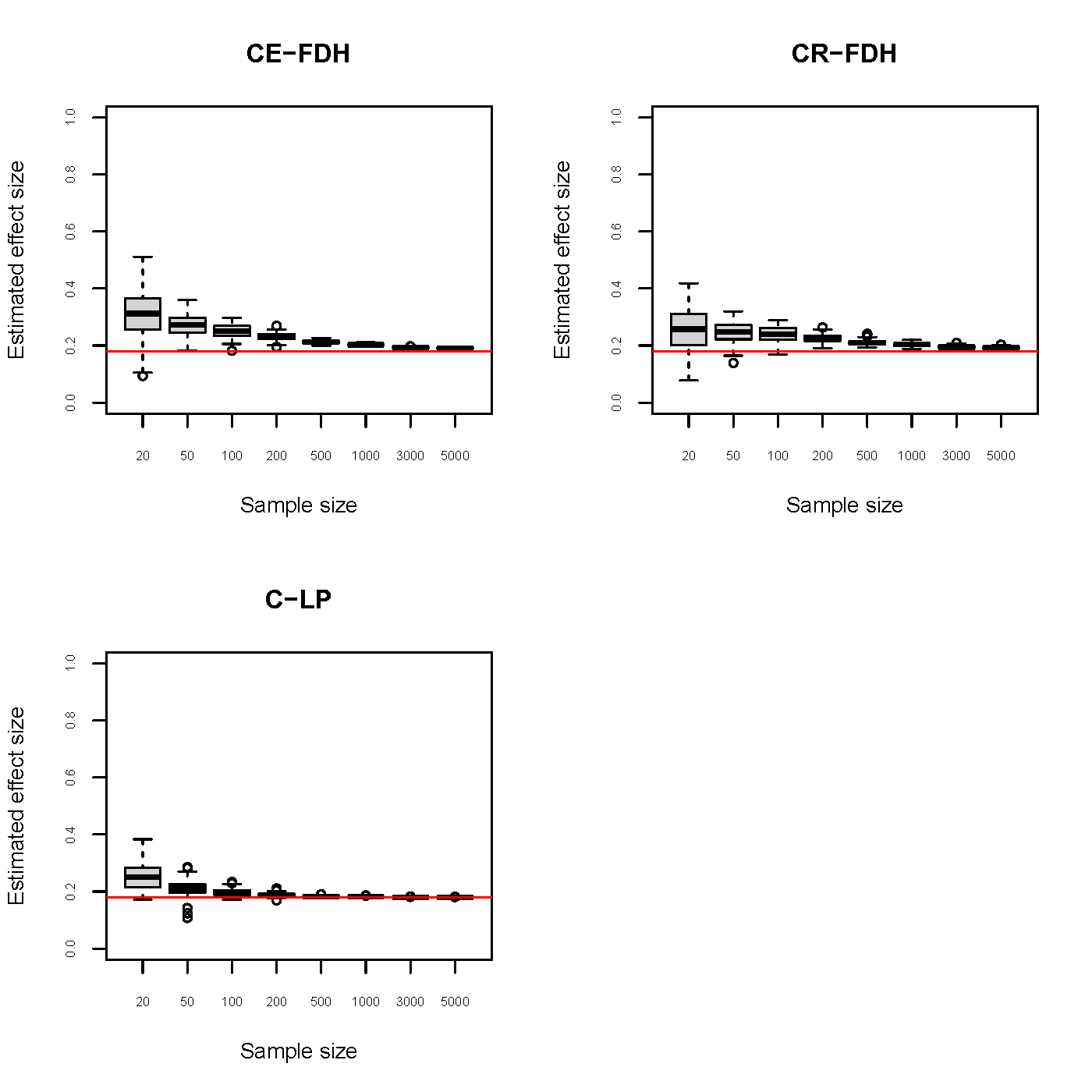
Figure 6.5: Monte Carlo simulation results for the effect size of three ceiling lines.True ceiling line = \(Y = 0.4 + X\). True effect size is 0.18.
Figure 6.5 suggests that for small samples the three ceiling lines are upward biased (the true effect size is smaller). When sample size increases, the estimated effect size approaches the true effect size (asymptotically unbiased) and the variance approaches zero. This means that the three estimators are consistent. C-LP and its effect size seems more efficient (less variation). These results only apply to the investigated conditions of a true ceiling line that is straight and there is no measurement error. Therefore, only when the true ceiling line is straight and when there is no measurement error the C-LP line may be preferred. Such ‘ideal’ circumstance may apply in simulation studies, but seldom in reality. When the true ceiling line is straight but cases have measurement error the CR-FDH line may perform better because measurement error usually reduces the effect size (ceiling line moves upwards). When the true ceiling line is not a straight line, CE-FDH may perform better because this this line can better follow the non-linearity of a the border (see Figure 3.9). Further simulations are needed to clarify the different statistical properties of the ceiling lines under different circumstances. In these simulations the effects of different population parameters (effect size, ceiling slope, ceiling intercept, non-linearity of the ceiling, distribution under the ceiling), and of measurement error (error-in-variable models) on the quality of the estimations could be studied.
6.3.4 Simulations of correlation
The correlation between two variables can me expressed as a number \(r\) , which is the correlation coefficient. This coefficient can have a value between -1 and +1. This section shows by simulations that a correlation between \(X\) and \(Y\) can be produced not only by a sufficiency relationship between \(X\) and \(Y\), but also by a necessity relationship. Correlation is not causation, and therefore an observed correlation cannot be automatically interpreted as in indication of sufficiency nor necessity.
6.3.4.1 Correlation by sufficiency
For empirical testing of a sufficiency relationship (e.g. as expressed in a hypothesis) the relationship is usually modeled as set of single factors (\(X\)’s) and possibly combinations of factors that add up to produce the outcome (additive logic). Such model captures a few factors of interest and assumes that all other factors together have on average no effect on the outcome. This sufficiency model corresponds to the well-known regression model with additive terms (with the factors of interest) and an error term (\(\epsilon\)) representing the other factors. Because the error term is assumed to have an average value of zero, the regression model with the factors of interest describes the average effect of these factors on the outcome. Note that it is often assumed that \(\epsilon\) is normally distributed and thus can have any value between minus Infinity and plus Infinity. As a consequence also \(Y\) can have any value between -Inf and + Inf. Moreover, the additive equation indicates that \(X\) is not a necessary cause of \(Y\) because a certain value of \(\epsilon\) can compensate for it.
A simple linear (average) sufficiency model is \(a + bx = y\), in which \(a\) is the intercept and \(b\) is the slope. The average sufficiency effect of \(X\) on \(Y\) can be modeled by the regression equation \(y = a + bx + \epsilon\). Figure 6.6 shows a \(XY\) scatter plot of 100 cases randomly from a population in which this linear relationship holds. \(X\) is a fixed variable between 0 and 1, and \(Y\) and \(\epsilon\) are normally distributed random variables with zero averages and standard deviations of 1. The simulation shows that the sufficiency relationship results in a correlation of 0.34.
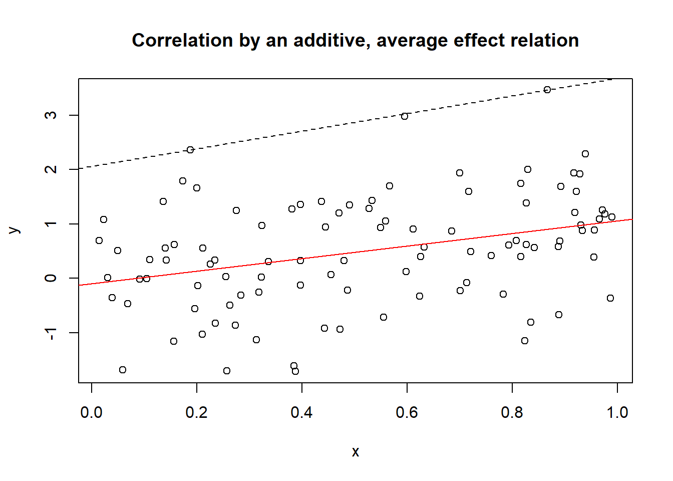
Figure 6.6: Correlation with coefficient 0.34 resulting from an average sufficiency relationship. The line through the middle is the regression line representing the sufficiency relationship.
The true (because induced) additive average sufficiency relationship in the population (in this case linear with parameters \(a = 0\) and \(b = 1\)) can be described with a regression line through the middle of the data (solid line). It would not be correct to draw a ceiling line on top of the data and interpret it as representing a necessity relationship between \(X\) and \(Y\) (dashed line).
6.3.4.2 Correlation by necessity
A necessity causal relationship between \(X\) and \(Y\) can also produce a correlation between \(X\) and \(Y\). For empirical testing of a necessity relationship (e.g. as expressed in a hypothesis) the relationship is modeled as a single factor that enables the outcome (necessity logic). Such model captures the single necessary factor independently of all other causal factors. This necessity model corresponds to the NCA ceiling line.
A simple linear necessity model (ceiling line) is \(a_c + b_cx = y\), in which \(a_c\) is the intercept of the ceiling line and \(b_c\) is the slope of the ceiling line that take values of 0.4 and 1 respectively. This can be represented by the ceiling equation \(y \leq a_c + b_cx\).
Figure 6.7 shows a \(XY\) scatter plot of 100 cases randomly selected from a population in which this linear ceiling relationship holds. \(X\) is a random variable between 0 and 1, and \(Y\) is a uniform distributed random variable bounded by the ceiling line. The simulation shows that the necessity relationship results in a correlation of 0.38.
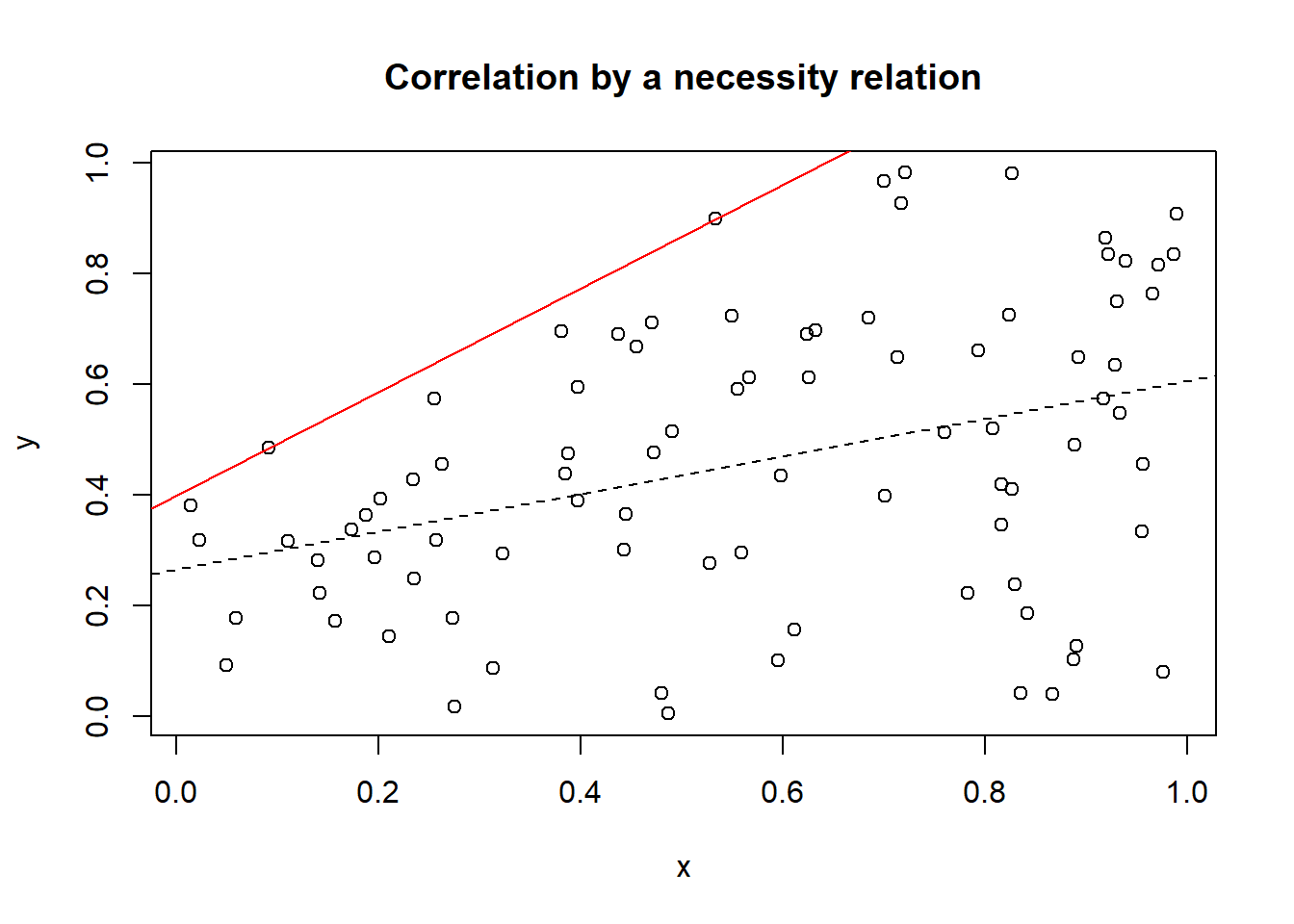
Figure 6.7: Correlation with coefficient 0.38 resulting from a necessity relationship. The line on top of the data is the ceiling line representing the necessity relationship.
The true (because induced) necessity relationship in the population (in this case linear ceiling with parameters \(a\) = 0.4 and \(b\) = 1) can be described with a ceiling line on top of the data (solid line). It would not be correct to draw a regression line through the middle of the data and interpret it as representing a sufficiency relationship between \(X\) and \(Y\) (dashed line).
6.3.4.3 Interpretation of correlation when causality is unknown
When the underlying causality is unknown the correlation coefficient cannot distinguish between the best way to describe it: by a regression line or by a ceiling line. A regression line can be added to the scatter plot when the underlying causality is assumed to be additive, average sufficiency logic, and the ceiling line can be added when the underlying causality is assumed to be necessity logic (or both).
The often implicit assumption that the correlation coefficient is caused by an underlying additive causal model may be wrong and may have two reasons. First, additive logic is the main paradigm of causality. Second, the correlation coefficient \(r\) and the regression coefficient \(b\) are closely related and can be expressed in a mathematical equation: \(r = b * sd(x)/sd(y)\) (\(sd\) is the standard deviation). A similar mathematical equation for the relationship between necessity effect size and correlation coefficient can be derived as well, but is very complex and not intuitive. (You can contact the author for this formulae with the assumption of a uniform distribution of the data below the ceiling line).
References
Note that standard bootstrapping should not be used, as the test statistic in NCA—the necessity effect size—does not satisfy the ‘smoothness’ assumption required for valid bootstrapping. Using bootstrapping with the necessity effect size may produce biased p values,↩︎