Chapter 1 Introduction to R
This chapter provides a brief introduction to the R programming language. The goal is to give just enough background to allow readers to move on quickly to the subsequent chapters, which focus on more advanced applications of R for geospatial data processing, analysis, and visualization. To understand and apply these techniques, it is essential to know the basic R objects that store various types of data. It is also necessary to understand how functions are used to manipulate these objects. Functions typically take one or more objects as inputs and modify them to produce a new object as the output. These concepts will be demonstrated by using R to perform a series of simple data processing tasks such as making basic calculations, applying these calculations over larger datasets, querying subsets of data that meet one or more conditions, creating graphics, and carrying out basic statistical tests.
1.1 Basic Calculations
The simplest way to use R is to type in a mathematical expression at the command prompt in the console and hit the Enter key. R will calculate the answer and print it on the screen. Alternatively, you can type the mathematical expressions as lines in an R script file. The code can then be run one line at a time using Ctrl+Enter on the keyboard or the Run button in the RStudio interface. Multiple lines can be run by highlighting them in the R script file and then using Ctrl+Enter or the Run button.
23 + 46
## [1] 69
27 * 0.003
## [1] 0.081
160 + 13 * 2.1
## [1] 187.3
(160 + 13) * 2.1
## [1] 363.3
It is strongly recommended that you work with R scripts from the outset rather than entering code directly into the console. Writing your code in a script file makes it easy to see the lines that have already been run, detect and correct any errors, and save the code so that you can share it or continue to work on it later. Eventually, you will develop more complex scripts with many lines of code to implement complex workflows. In RStudio, you can create a new script file by selecting File > New File > R Script from the RStudio menu or using the Ctrl+Shift+N key combination. Script files can be saved and opened using the File menu in RStudio or with keyboard shortcuts such as Ctrl+O to open and Ctrl+S to save.
Instead of just printing the results on the screen, the outputs of mathematical expressions can be saved as variables using the leftward assignment operator (<-). Creating variables allows information to be stored and reused at a later time. R stores each variable as an object.
x <- 15
x
## [1] 15
y <- 23 + 15 / 2
y
## [1] 30.5
z <- x + y
z
## [1] 45.5
A single equal sign, =, can also be used as an assignment operator in R like in many other programming languages. This book exclusively uses the <- operator for clarity. The single equal sign is also used in R to associate function arguments with values, which can lead to ambiguity and confusion. It is also easy to confuse the = assignment operator with the == logical operator.
When an object name is entered at the command line or through a script, R will invoke the print() function and output information about the object to the console. The print() function is an example of a generic function that can take a variety of object classes as input. Each class has an associated method that determines how it will be printed. Thus, a generic function like print() will produce different results depending on the characteristics of the input.
The R console is used to get “quick looks” at the data and analysis results. However, the text format of the console greatly limits what can be displayed. In addition to printing results to the screen, they can also be exported as tables, figures, and new datasets using the techniques that will be covered in this book.
1.2 R Objects
1.2.1 Vectors
When working with real data, it is necessary to keep track of sets of numbers that represent different types of measurements. Therefore, the fundamental type of object in R is a vector, which can contain multiple values. The single-value objects created in the previous section were actually vectors with a length of one.
As a more realistic example, consider data on forest canopy cover (the percent of the sky that is obscured by tree leaves, branches, and boles as seen from the ground) collected in the field. Data are usually collected from multiple field plots, and each plot may be revisited and resampled multiple times. We will start by creating a small dataset with 12 measurements of forest cover. The c() (combine) function is used to create a vector object named cover that contains these data. Any number of comma-separated data values can be provided as arguments to c().
cover <- c(63, 86, 23, 77, 68, 91, 43, 76, 69, 12, 31, 78)
cover
##  [1] 63 86 23 77 68 91 43 76 69 12 31 78
An important element of coding in R (or any other programming language) is selecting names for the objects that are created. In R, object names must begin with a letter or a period, must contain only letters, numbers, underscores, and dots, and should not conflict with the names of R keywords and functions. For example, objects should never be named c because this name conflicts with the c() function.
It is up to the user to specify object names. Try to choose descriptive abbreviations that will help you remember the information contained in your R objects. However, variable names should not be so lengthy that they are cumbersome to read and type. In this case, cover is a simple and straightforward name to use, but cc or cancov or even canopy_cover would also be suitable depending on the programmer’s preferences.
There are several widely used conventions for formatting object names, and it is best to select one and use it consistently. For example, consider an R object that will store topographic measurements of slope angle in radians. Some names based on commonly used case types include slopeRad (camel case), slope_rad (snake case), slope-rad (kebab case), and SlopeRad (Pascal case). Most of the code in this book is written in snake case, because this is the style that the author learned when he started programming many years ago. The particular variable case that you choose matters less than applying it consistently and choosing good variable names.
Several functions can be used to create vectors containing regular sequences of numbers or repeated values. The seq() function generates a sequence of numbers from a beginning number to another number with values separated by a specified amount.
seq(from=1, to=12, by=1)
##  [1]  1  2  3  4  5  6  7  8  9 10 11 12
seq(from=10, to=100, by=10)
##  [1]  10  20  30  40  50  60  70  80  90 100
The colon operator (:) can also be used to generate integer sequences between two numbers.
1:10
##  [1]  1  2  3  4  5  6  7  8  9 10
37:41
## [1] 37 38 39 40 41
The rep() function takes a vector and repeats the entire vector a specified number of times, or repeats each value in the vector.
rep(5, times=4)
## [1] 5 5 5 5
s1 <- 1:4
rep(s1, times=4)
##  [1] 1 2 3 4 1 2 3 4 1 2 3 4 1 2 3 4
rep(s1, each=3)
##  [1] 1 1 1 2 2 2 3 3 3 4 4 4
These examples provide a first look at how R functions work. One or more arguments are specified to determine the sequences that are generated, and the function outputs a vector. Because the function output is not assigned to an object, it is printed to the screen by default. We will discuss functions in more detail and look at some more complex examples later in the chapter.
Continuing with the canopy cover example, assume that there are four plots are coded 1, 2, 3, and 4 and each plot was measured in 2014, 2015, and 2016. The following code creates vectors containing the plot codes and years corresponding to each set of canopy cover observations.
plots <- 1:4
plot_codes <- rep(plots, times=3)
years <- rep(2014:2016, each=4)
plot_codes
##  [1] 1 2 3 4 1 2 3 4 1 2 3 4
years
##  [1] 2014 2014 2014 2014 2015 2015 2015 2015 2016 2016 2016
## [12] 2016
One of the most important features of R is that it uses vector arithmetic to carry out element-wise mathematical operations without having to write code for looping. If a mathematical operation is performed on two or more vectors of equal length, the operation will be carried out on the elements of each vector in sequence, returning a vector of the same length as the inputs. If one input is a single value and another is a longer vector, the single value will automatically be repeated for the entire length of the longer vector. Thus, the following two statements produce the same output.
cover + cover
##  [1] 126 172  46 154 136 182  86 152 138  24  62 156
cover * 2
##  [1] 126 172  46 154 136 182  86 152 138  24  62 156
Some additional examples of vector arithmetic are provided below. They add the same scalar to each canopy cover value, convert the canopy cover from percentage to proportion, and compute the mean of three canopy cover measurements for each combination of plot and year.
cover + 5
##  [1] 68 91 28 82 73 96 48 81 74 17 36 83
cover / 100
##  [1] 0.63 0.86 0.23 0.77 0.68 0.91 0.43 0.76 0.69 0.12 0.31
## [12] 0.78
cover2 <- c(59, 98, 28, 71, 62, 90, 48, 77, 74, 15, 38, 75)
cover3 <- c(91, 91, 33, 68, 59, 88, 44, 81, 72, 23, 44, 67)
tot_cover <- cover + cover2 + cover3
mean_cover <- tot_cover / 3
mean_cover
##  [1] 71.00000 91.66667 28.00000 72.00000 63.00000 89.66667
##  [7] 45.00000 78.00000 71.66667 16.66667 37.66667 73.33333
Vectors can also be supplied as arguments to functions to compute statistics such as the mean, sum, variance, and length. The examples below show how to use functions to calculate the sum, mean, and variance of canopy cover as well as the total number of values in the vector.
sum(cover)
## [1] 717
mean(cover)
## [1] 59.75
var(cover)
## [1] 678.3864
length(cover)
## [1] 12
The following examples show how vector operations can be used to calculate the mean and variance. The mean is the sum of the canopy cover values divided by the number of observations. The variance is the sum of square differences of each canopy cover and the mean canopy cover divided by the number of observations minus one.
meancover <- sum(cover) / length(cover)
meancover
## [1] 59.75
varcover <- sum((cover - meancover)^2) / (length(cover)-1)
varcover
## [1] 678.3864
Subsets of data can be selected by specifying one or more index numbers within square brackets. These index numbers are also referred to as subscripts. Positive numbers are used to include subsets in the output, and negative numbers are used to exclude subsets.
cover[1]
## [1] 63
cover[10]
## [1] 12
cover[c(1, 3, 8, 11)]
## [1] 63 23 76 31
cover[9:12]
## [1] 69 12 31 78
cover[-2]
##  [1] 63 23 77 68 91 43 76 69 12 31 78
Up to this point, we have been working with vectors that contain numerical values. However, vectors can also belong to different classes that contain other types of information. For example, logical vectors have only two possible values (TRUE and FALSE) and belong to a different object class than the numeric vectors that we have been working with so far. Logical vectors can be used to select subsets that meet certain criteria. Here, a logical vector that indicates which observations have canopy cover values greater than 50% is generated. Then the logical vector is used to extract the subset of canopy cover observations greater than 50%. The class() function returns the object class to which the vector belongs.
class(cover)
## [1] "numeric"
cov_gt50 <- cover > 50
cov_gt50
##  [1]  TRUE  TRUE FALSE  TRUE  TRUE  TRUE FALSE  TRUE  TRUE
## [10] FALSE FALSE  TRUE
class(cov_gt50)
## [1] "logical"
cover[cov_gt50]
## [1] 63 86 77 68 91 76 69 78
The logical expression can also be nested inside the brackets to extract the subset using a single line of code.
high_cov <- cover[cover > 50]
high_cov
## [1] 63 86 77 68 91 76 69 78
In addition to numeric and logical vectors, vectors can also be composed of character data such as place names and plot codes.
plot_name <- c("Plot A4", "Plot A16", "Plot B2", "Plot B5", "Plot C11")
length(plot_name)
## [1] 5
class(plot_name)
## [1] "character"
There is also a special type of vector called a factor that is used for categorical data. To use the vector of plot names in an analysis comparing statistics across the different plots, it first needs to be converted into a factor. There are many more nuances to factors, but for now, it is sufficient to know that the factor object contains a levels attribute that specifies its categories.
plot_fact <- factor(plot_name)
class(plot_fact)
## [1] "factor"
plot_name
## [1] "Plot A4"  "Plot A16" "Plot B2"  "Plot B5"  "Plot C11"
plot_fact
## [1] Plot A4  Plot A16 Plot B2  Plot B5  Plot C11
## Levels: Plot A16 Plot A4 Plot B2 Plot B5 Plot C11
Numerical vectors can also be converted to factors. For example, there are some situations where plot numbers or years need to be treated as categories rather than continuous numerical measurements. The following code overwrites the plot_codes and year objects, effectively converting them from numeric vectors to factors.
plot_codes
##  [1] 1 2 3 4 1 2 3 4 1 2 3 4
years
##  [1] 2014 2014 2014 2014 2015 2015 2015 2015 2016 2016 2016
## [12] 2016
plot_codes <- factor(plot_codes)
years <- factor(years)
plot_codes
##  [1] 1 2 3 4 1 2 3 4 1 2 3 4
## Levels: 1 2 3 4
years
##  [1] 2014 2014 2014 2014 2015 2015 2015 2015 2016 2016 2016
## [12] 2016
## Levels: 2014 2015 2016
The NA symbol is a special value used in R to indicate missing data. When processing and managing data, it is critical that missing data be appropriately flagged as NA rather than treated as zero or some other arbitrary value. Most R functions have built-in techniques for handling missing data, and as we will see in later examples, the user must often choose the appropriate technique for a particular analysis.
In the example below, a vector is created containing four numerical values and two NA codes. The is.na() function returns a vector of logical values indicating whether or not each element in the vector is NA. Because logical values of TRUE and FALSE have equivalent numerical values of 1 and 0, summing the logical vector returns the total number of NA values.
myvector <- c(2, NA, 9, 2, 1, NA)
is.na(myvector)
## [1] FALSE  TRUE FALSE FALSE FALSE  TRUE
sum(is.na(myvector))
## [1] 2
By default, many functions will return NA if the input data contain NA values. When the na.rm argument is set to TRUE, the NA values are removed and the mean is computed using only the valid observations.
mean(myvector)
## [1] NA
mean(myvector, na.rm = TRUE)
## [1] 3.5
Dealing with missing data is an important aspect of most data science workflows. A common mistake is to assume that missing data are equivalent to a zero value. For example, rainfall observations may be missing from a meteorological datasets for several weeks because of an equipment malfunction or data loss. However, it should not be assumed that no rainfall occurred during these weeks just because no measurements were taken. Missing data should always be specified as NA in R, which will allow the analyst to identify them and take appropriate steps to account for them when summarizing and analyzing the data.
1.2.2 Matrices and Lists
Multiple vectors of the same length can be combined to create a matrix, which is a two-dimensional object with columns and rows. All of the values in a matrix must be the same data type (e.g., numeric, character, or logical). The cbind() function combines the vectors as columns and the rbind() function combines the vectors as rows. There is also a matrix() function that reformats data from a vector into a matrix. The dim() function returns the number of rows and columns in the matrix.
mat1 <- cbind(cover, cover2, cover3)
mat1
##       cover cover2 cover3
##  [1,]    63     59     91
##  [2,]    86     98     91
##  [3,]    23     28     33
##  [4,]    77     71     68
##  [5,]    68     62     59
##  [6,]    91     90     88
##  [7,]    43     48     44
##  [8,]    76     77     81
##  [9,]    69     74     72
## [10,]    12     15     23
## [11,]    31     38     44
## [12,]    78     75     67
class(mat1)
## [1] "matrix" "array"
dim(mat1)
## [1] 12  3
Subsets of matrix elements can be extracted by providing row and column indices in [row, column].
mat1[1,1]
## cover
##    63
Leaving one of these values blank will return all rows or columns, as shown in the examples below.
mat1[1:3,]
##      cover cover2 cover3
## [1,]    63     59     91
## [2,]    86     98     91
## [3,]    23     28     33
mat1[,2]
##  [1] 59 98 28 71 62 90 48 77 74 15 38 75
Lists are ordered collections of objects. They are created using the list() function and elements can be extracted by index number or component name. Lists differ from vectors and matrices in that they can contain a mixture of different data types. The example below creates a two-element list containing a vector and a matrix.
l1 <- list(myvector = cover, mymatrix = mat1)
l1
## $myvector
##  [1] 63 86 23 77 68 91 43 76 69 12 31 78
##
## $mymatrix
##       cover cover2 cover3
##  [1,]    63     59     91
##  [2,]    86     98     91
##  [3,]    23     28     33
##  [4,]    77     71     68
##  [5,]    68     62     59
##  [6,]    91     90     88
##  [7,]    43     48     44
##  [8,]    76     77     81
##  [9,]    69     74     72
## [10,]    12     15     23
## [11,]    31     38     44
## [12,]    78     75     67
List elements can be extracted by providing either an element number or name inside of double brackets.
l1[[1]]
##  [1] 63 86 23 77 68 91 43 76 69 12 31 78
l1[["myvector"]]
##  [1] 63 86 23 77 68 91 43 76 69 12 31 78
List elements can also be extracted using the $ operator followed by the element name.
l1$myvector
##  [1] 63 86 23 77 68 91 43 76 69 12 31 78
1.2.3 Data Frames
Data frames are like matrices in that they have a rectangular format consisting of columns and rows, and they are like lists in that they can contain columns with different data types such as numeric, logical, character, and factor. In general, the rows of a data frame represent observations (e.g., measurements taken at different locations and times), whereas the columns contain descriptive labels and variables for each observation.
The example below uses the data.frame() function to create a simple data frame consisting of three different canopy cover measurements taken at four plots for three years (12 observations total). The attributes() function returns the dimensions of the data frame along with the variable names.
cover_data <- data.frame(plot_codes, years, cover, cover2, cover3)
attributes(cover_data)
## $names
## [1] "plot_codes" "years"      "cover"      "cover2"
## [5] "cover3"
##
## $class
## [1] "data.frame"
##
## $row.names
##  [1]  1  2  3  4  5  6  7  8  9 10 11 12
The summary() function returns an appropriate statistical summary of each variable in the data frame. For columns of factors such as plot_codes, the counts of observations correponding to each level are displayed. For columns of numerical data such as cover, several summary statistics are provided to describe the distribution of the values.
summary(cover_data)
##  plot_codes  years       cover           cover2
##  1:3        2014:4   Min.   :12.00   Min.   :15.00
##  2:3        2015:4   1st Qu.:40.00   1st Qu.:45.50
##  3:3        2016:4   Median :68.50   Median :66.50
##  4:3                 Mean   :59.75   Mean   :61.25
##                      3rd Qu.:77.25   3rd Qu.:75.50
##                      Max.   :91.00   Max.   :98.00
##      cover3
##  Min.   :23.00
##  1st Qu.:44.00
##  Median :67.50
##  Mean   :63.42
##  3rd Qu.:82.75
##  Max.   :91.00
The columns of a data frame can be accessed like list elements with the $ operator.
cover_data$plot_codes
##  [1] 1 2 3 4 1 2 3 4 1 2 3 4
## Levels: 1 2 3 4
cover_data$cover
##  [1] 63 86 23 77 68 91 43 76 69 12 31 78
Values in data frames can also be accessed using matrix-style indexing of rows and columns.
cover_data[3, 4]
## [1] 28
cover_data[1:3,]
##   plot_codes years cover cover2 cover3
## 1          1  2014    63     59     91
## 2          2  2014    86     98     91
## 3          3  2014    23     28     33
cover_data[,4]
##  [1] 59 98 28 71 62 90 48 77 74 15 38 75
cover_data[,"cover2"]
##  [1] 59 98 28 71 62 90 48 77 74 15 38 75
Conditional statements can be used to query data records meeting certain conditions. Note that when referencing columns of a data frame, it is necessary to specify the data frame and reference the columns using the $ operator.
cover_data[cover_data$years == 2015,]
##   plot_codes years cover cover2 cover3
## 5          1  2015    68     62     59
## 6          2  2015    91     90     88
## 7          3  2015    43     48     44
## 8          4  2015    76     77     81
cover_data[cover_data$cover > 70,]
##    plot_codes years cover cover2 cover3
## 2           2  2014    86     98     91
## 4           4  2014    77     71     68
## 6           2  2015    91     90     88
## 8           4  2015    76     77     81
## 12          4  2016    78     75     67
A conditional statement based on the & (logical and) operator requires that both conditions are met
cover_data[cover_data$cover > 70 & cover_data$cover3 > 70,]
##   plot_codes years cover cover2 cover3
## 2          2  2014    86     98     91
## 6          2  2015    91     90     88
## 8          4  2015    76     77     81
A conditional statement based on the | (logical or) operator requires that at least one of the conditions is met.
cover_data[cover_data$cover > 70 | cover_data$cover3 > 70,]
##    plot_codes years cover cover2 cover3
## 1           1  2014    63     59     91
## 2           2  2014    86     98     91
## 4           4  2014    77     71     68
## 6           2  2015    91     90     88
## 8           4  2015    76     77     81
## 9           1  2016    69     74     72
## 12          4  2016    78     75     67
1.3 R Functions
An R function takes one or more arguments as inputs and produces an object as the output. Thus far, a variety of relatively simple functions have been used to do basic data manipulation and print results to the console. Moving forward, the key to understanding how to do more advanced geospatial data processing, visualization, and analysis in R is learning which functions to use and how to specify the appropriate arguments for those functions. This section will illustrate the use of some functions to generate basic graphics and carry out standard statistical analyses.
1.3.1 Data Input and Graphics
Data are imported from an external file named "camp32.csv", which contains data in a comma-delimited format. The read.csv() function reads in the file and outputs to a data frame, which is stored as an object called camp32_data. The file argument indicates the name of the file to read. Make sure this file is in your working directory so that it can be read without specifying any additional information about its location. The most straightforward way to do this is to create an R project associated with a specific folder in your computer’s file system. Then copy your input files to this folder and it will become the default location for file input and output. See the section in the Appendix on Managing RStudio Projects for more details.
camp32_data <- read.csv(file = "camp32.csv")
summary(camp32_data)
##      DATE             PLOT_ID               LAT
##  Length:36          Length:36          Min.   :48.84
##  Class :character   Class :character   1st Qu.:48.85
##  Mode  :character   Mode  :character   Median :48.85
##                                        Mean   :48.85
##                                        3rd Qu.:48.85
##                                        Max.   :48.86
##       LONG             DNBR            CBI
##  Min.   :-115.2   Min.   :-34.0   Min.   :0.780
##  1st Qu.:-115.2   1st Qu.: 85.5   1st Qu.:1.302
##  Median :-115.2   Median :298.0   Median :2.125
##  Mean   :-115.2   Mean   :333.2   Mean   :1.906
##  3rd Qu.:-115.2   3rd Qu.:561.0   3rd Qu.:2.485
##  Max.   :-115.2   Max.   :771.0   Max.   :2.700
##   PLOT_CODE
##  Length:36
##  Class :character
##  Mode  :character
##
##
##
These data include field and remote sensing measurements of wildfire severity for a set of plots on the Camp 32 fire in northwestern Montana. Higher values of the wildfire severity indices generally indicate that a higher proportion of trees were damaged or killed by the fire. Some of the plots were subjected to fuel treatments that removed overstory trees by mechanical thinning, reduced live and dead surface fuels with low-severity prescribed burns, or combined thinning and prescribed burning. Visualizing and analyzing these data can allow us to see whether these treatments moderated the effects of the wildfire. More information about the Camp32 fire and the data are available in (Michael C. Wimberly et al. 2009).
The following data columns will be used.
- CBI: Composite Burn Index, a field-measured index of fire severity
- DNBR: Difference Normalized Burn Ratio, a remotely sensed index of fire severity
- PLOT_CODE: Fuel treatments that were implemented before the wildfire, U=untreated, T=thinning, TB=thinning and prescribed burning
One question is whether the field-based and satellite-based metrics provide similar information about wildfire severity. We can explore this by using the plot() function to generate a scatterplot of CBI versus DNBR. Two vectors of data are specified as the x and y arguments. Note that the $ operator must be used to access the columns of the camp32_data data frame. The result shows that there is a relatively strong associations between these two variables and suggests that the relationship may be non-linear (Figure 1.1).
plot(x = camp32_data$CBI, y = camp32_data$DNBR)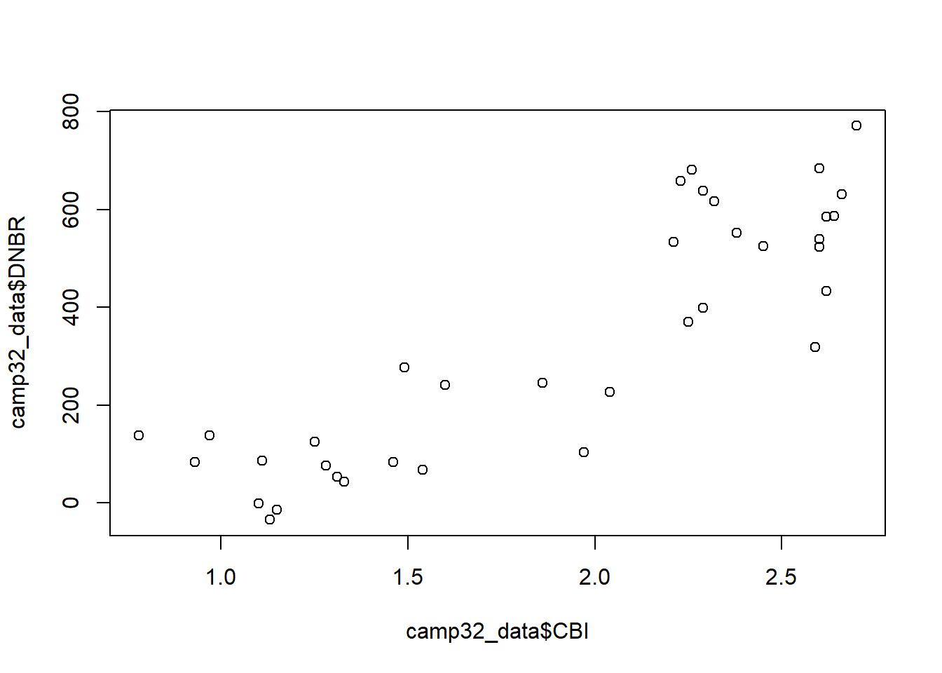
FIGURE 1.1: Scatterplot of the CBI and DNBR fire severity indices.
When a plotting function is run, its output is sent to a graphical device. In RStudio, the built-in graphical device is located in the lower right-hand pane in the Plots tab. The plot can be copied or saved to a graphics file using the Export button, and it can be expanded using the Zoom button.
To make a more interpretable plot, a title and axis labels can be specified as additional arguments to the plot() function (Figure 1.2).
plot(x = camp32_data$CBI, y = camp32_data$DNBR,
     main = "Camp 32 Fire Severity",
     xlab = "CBI",
     ylab = "DNBR")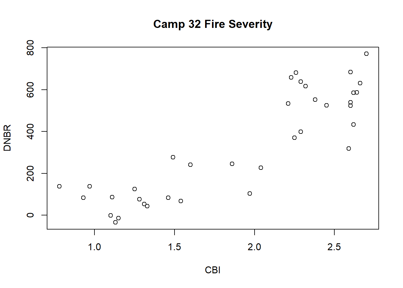
FIGURE 1.2: Scatterplot of the CBI and DNBR fire severity indices with axis labels and title.
At this initial data exploration stage, it is also helpful to explore the distributions of the variables of interest using histograms. The hist() function is used in this example to create a histogram of the DNBR values (Figure 1.3). Because a histogram is a univariate plot, only a single vector of data is provided as the x argument along with a title and x-axis label.
hist(x = camp32_data$DNBR,
     main = "Differenced Normalized Burn Ratio",
     xlab = "DNBR")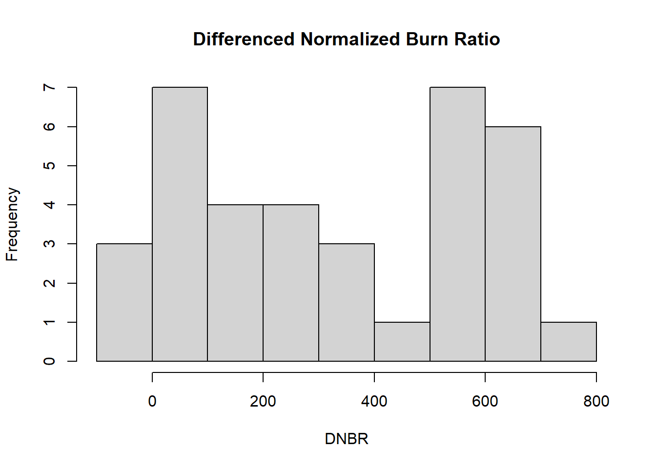
FIGURE 1.3: Histogram of the DNBR fire severity index.
A boxplot can be used to visualize the distributions of fire severity in plots with different types of fuel treatments. The boxplot() function generates this plot, and the arguments used here are different from the preceding examples. The first argument is a formula, DNBR ~ PLOT_CODE, where the value to the left of the ~ (tilde) operator is the dependent variable and one or more values on the right-hand side are independent variables. The data argument specifies the data frame containing these columns, and additional arguments provide a title and axis labels. Compared to the untreated plots, the thinned plots have slightly higher DNBR, whereas the thinned and burned plots have much lower DNBR (Figure 1.4).
boxplot(formula = DNBR ~ PLOT_CODE,
        data = camp32_data,
        main = "Treatment Effects on Fire Severity",
        xlab = "Treatment Type",
        ylab = "DNBR")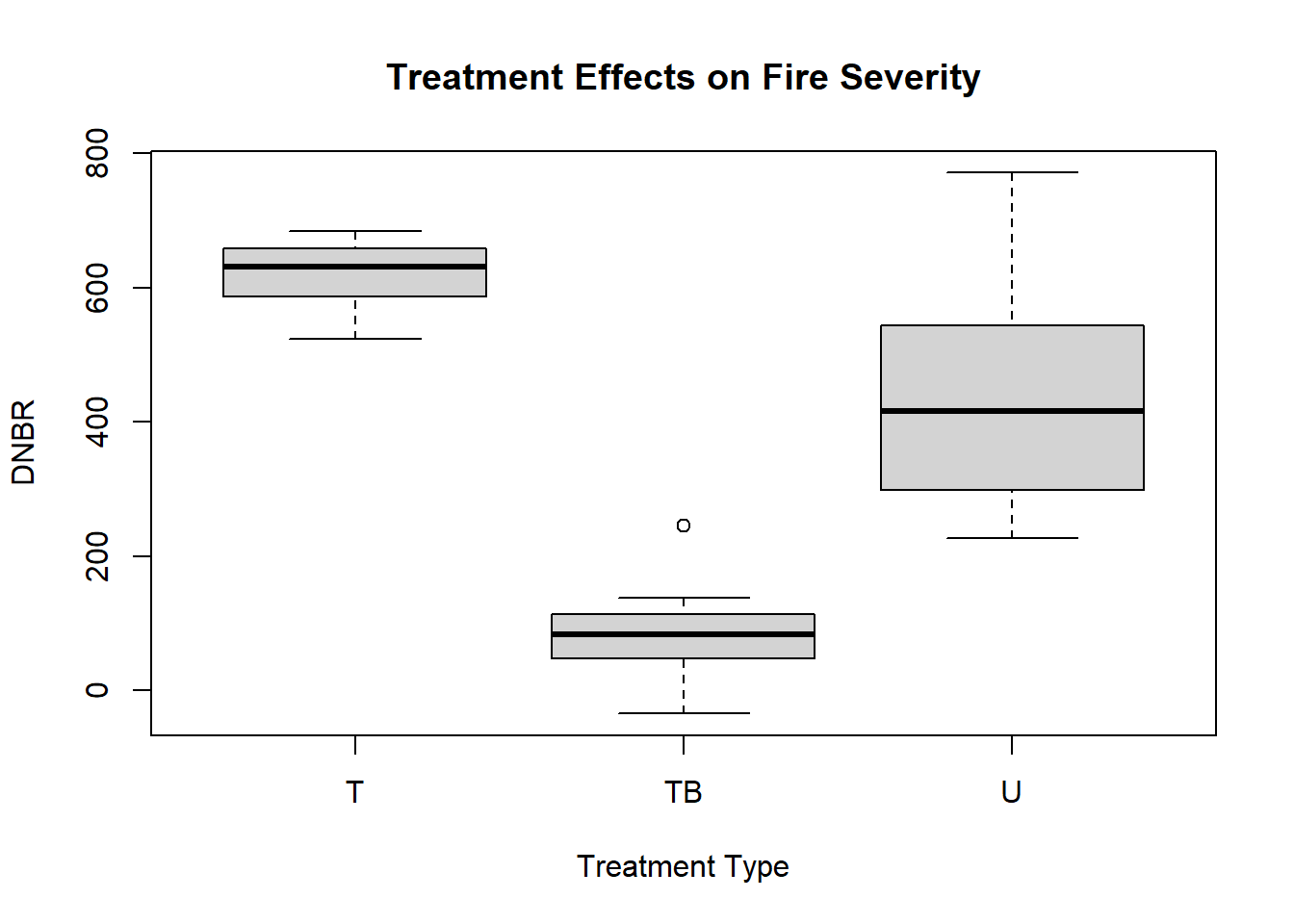
FIGURE 1.4: Boxplot showing the distribution of the DNBR fire severity index.
Knowing the arguments that can be specified for a specific function is very important. The quickest way to learn more about an R function is to display its documentation using the help() function. This function provides access to manual pages with information about function arguments, details about what the function does, and a description of the output that is produced. In RStudio, the help pages are displayed in the Help tab in the lower right-hand window.
help(plot)
help(hist)
help(boxplot)
1.3.2 Statistical Analysis
Functions are also used to carry out statistical tests in R. For example, the t.test() function can be used to compute confidence intervals for the mean of a variable. The x argument is the vector of data to summarize. The output of the function is an object of class htest that contains information about the results of the statistical test. When the output of a function like t.test() is not assigned to an object as in the following examples, the print() function is invoked for the resuting htest object. The print() method for this object class generates a summary of the statistical test results and outputs them to the console.
t.test(x = camp32_data$DNBR)
##
##  One Sample t-test
##
## data:  camp32_data$DNBR
## t = 7.963, df = 35, p-value = 2.286e-09
## alternative hypothesis: true mean is not equal to 0
## 95 percent confidence interval:
##  248.2493 418.1396
## sample estimates:
## mean of x
##  333.1944
The conf.level argument can be used to specify the probability association with the confidence intervals. Note that in the previous example, no conf.level argument was provided, but a 95% confidence interval was produced.
t.test(x=camp32_data$DNBR, conf.level=0.9)
##
##  One Sample t-test
##
## data:  camp32_data$DNBR
## t = 7.963, df = 35, p-value = 2.286e-09
## alternative hypothesis: true mean is not equal to 0
## 90 percent confidence interval:
##  262.4982 403.8907
## sample estimates:
## mean of x
##  333.1944
How does the t.test() function know what confidence level to use if we do not specify the conf.level argument? In many cases, arguments have a default value. If the argument is not specified in the function call, then the default value is used. When using statistical functions in R, it is particularly important to study the documentation to learn the default values and decide if they are appropriate for the analysis. The default values are specified at the beginning of the function’s help page in the usage section.
help(t.test)A two-sample t-test can be used to compare the mean DNBR values for treated versus untreated plots. The same function is used with two arguments, x and y, which are the two vectors of data to be compared. In the code below, two new vectors are created from the camp32_data data frame. U_DNBR contains DNBR values from the untreated plots and TB_DNBR contains DNBR values from the thinned and burned plots. Within the square brackets, the logical statement to the left of the comma specifies which rows to include, the character string to the right of the comma specifies which column to include.
U_DNBR <- camp32_data[camp32_data$PLOT_CODE == "U", "DNBR"]
TB_DNBR <- camp32_data[camp32_data$PLOT_CODE == "TB", "DNBR"]
t.test(x=U_DNBR, y=TB_DNBR)
##
##  Welch Two Sample t-test
##
## data:  U_DNBR and TB_DNBR
## t = 7.0902, df = 14.174, p-value = 5.058e-06
## alternative hypothesis: true difference in means is not equal to 0
## 95 percent confidence interval:
##  248.8065 464.2602
## sample estimates:
## mean of x mean of y
##  436.3333   79.8000
A linear regression analysis can be used to explore the relationship between the field-based burn severity index (CBI) and the satellite-derived burn severity index (DNBR). Ordinary least squares regression is implemented with the lm() function. This function requires at least two arguments, a formula and a data argument, and returns an object belonging to class lm. Note that lm objects, like the htest objects produced by t.test() are really list objects whose elements contain various pieces of information about the analysis results. The names of these elements can be obtained using the attributes() function.
camp32_lm <- lm(formula = CBI ~ DNBR,
                data = camp32_data)
class(camp32_lm)
## [1] "lm"
attributes(camp32_lm)
## $names
##  [1] "coefficients"  "residuals"     "effects"
##  [4] "rank"          "fitted.values" "assign"
##  [7] "qr"            "df.residual"   "xlevels"
## [10] "call"          "terms"         "model"
##
## $class
## [1] "lm"
To obtain more interpretable results, additional functions are needed to summarize the lm object. In this case, the print() method displays only the original function and the regression coefficients. There is also a generic summary() function.
camp32_lm
##
## Call:
## lm(formula = CBI ~ DNBR, data = camp32_data)
##
## Coefficients:
## (Intercept)         DNBR
##    1.178530     0.002183
For lm objects, the summary() method provides much more detail, including statistical tests for the coefficients and the overall model as well as the R2 measure of model fit. Here, the R2 value of 0.76 indicates a moderately strong association between these two indices.
summary(camp32_lm)
##
## Call:
## lm(formula = CBI ~ DNBR, data = camp32_data)
##
## Residuals:
##      Min       1Q   Median       3Q      Max
## -0.69976 -0.20237  0.00781  0.18838  0.71515
##
## Coefficients:
##              Estimate Std. Error t value Pr(>|t|)
## (Intercept) 1.1785297  0.0867154   13.59 2.66e-15 ***
## DNBR        0.0021828  0.0002089   10.45 3.75e-12 ***
## ---
## Signif. codes:
## 0 '***' 0.001 '**' 0.01 '*' 0.05 '.' 0.1 ' ' 1
##
## Residual standard error: 0.3103 on 34 degrees of freedom
## Multiple R-squared:  0.7625, Adjusted R-squared:  0.7555
## F-statistic: 109.2 on 1 and 34 DF,  p-value: 3.746e-12
The fitted values and residuals of the regression model can be extracted using the fitted() and resid() functions. The scatterplot of these variables is a common diagnostic of model fit (Figure 1.5). In this case, the arched shape of the point cloud indicates nonlinearity in the relationship between the two severity indices.
plot(x = fitted(camp32_lm), y = resid(camp32_lm),
     xlab = "Fitted Values",
     ylab = "Residuals")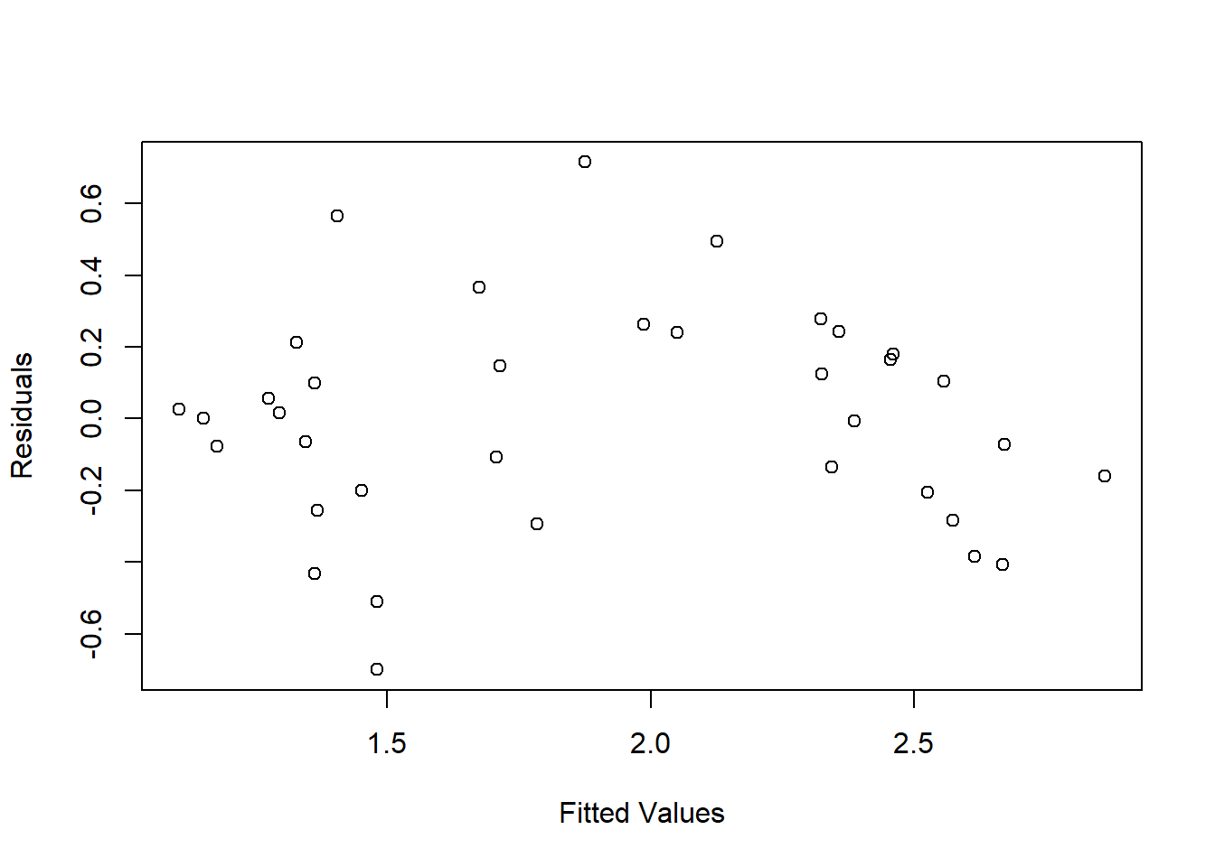
FIGURE 1.5: Scatterplot of residuals versus fitted values from linear regression of CBI versus DNBR.
1.4 Tips for Programming in R
The following block of code contains several lines that begin with a hash symbol (#) followed by descriptive text. Whenever the R interpreter encounter the # symbol, the rest of that line is ignored. Therefore, # is used to indicate comment lines that contain descriptive text rather than interpretable code. Whether writing code in R or other computer languages, it is essential to include descriptive comments that explain what the code is intended to do and how it is expected to work. Comments are particularly important if you intend to revisit and reuse or code at some point in the future, or share it with others to use and modify. Most of the code presented in this book does not include comments. This is intended to save space and increase readability, as explanations of the code are already provided in the accompanying text. In later chapters, there will be some examples of how comments can be used to organize and document R scripts that implement longer and more complicated analytical workflows.
###########################################################
# Example R script demonstrating the use of comments
###########################################################

# Read in fire severity data comma-delimited file
camp32_data <- read.csv(file = "camp32.csv")
# Box plot of DNBR distributions for different treatments
boxplot(formula = DNBR ~ PLOT_CODE,
        data = camp32_data,
        main = "Treatment Effects on Fire Severity",
        xlab = "Treatment Type",
        ylab = "DNBR")
# Extract vectors of untreated and thinned/burned DNBR
U_DNBR <- camp32_data[camp32_data$PLOT_CODE == "U", "DNBR"]
TB_DNBR <- camp32_data[camp32_data$PLOT_CODE == "TB", "DNBR"]
# t-test with null hypothesis of equal means
t.test(x=U_DNBR, y=TB_DNBR)
# Linear regression of CBI versus DNBR
camp32_lm <- lm(formula = CBI ~ DNBR,
                data = camp32_data)
summary(camp32_lm)
# Residuals versus fitted values diagnostic plot
plot(x = fitted(camp32_lm), y = resid(camp32_lm),
     xlab = "Fitted Values",
     ylab = "Residuals")
1.5 Practice
Create two new vectors, one containing all the odd numbers between 1 and 19, and the other containing all even numbers between 2 and 20. Add the two vectors element-wise to produce a single vector and then create a new vector that contains only numbers greater than 15. Finally, compute the mean value of this vector. If you do all the calculations right, the mean will equal 29.
Starting with the cover_data data frame, create a new data frame containing only the rows of data for plot number 3 and print the results to the screen.
From the Camp 32 dataset, extract a vector containing the CBI values from the untreated plots (treatment code U) and another containing the CBI values for the thinned/unburned plots (treatemnt code T). Conduct a two-sample t-test comparing the mean CBI for these two treatment types.
Generate a histogram plot of CBI values and compare it with the histogram of DNBR values.
Generate a new scatterplot based on the observed values of CBI on the x-axis and the predicted values of CBI from the linear regression on the y-axis. Make the plot have an aspect ratio of 1 (equal scales of x and y axes). To do this, you will need to specify an additional argument. Consult the help page for the base
plot()function to find the name of the argument to use.