Chapter 8 Coordinate Reference Systems

All geospatial data have a coordinate reference system (CRS) that defines how the two-dimensional coordinates used for mapping and analysis are related to real locations on the Earth’s surface. Important components of the CRS include the ellipsoid that models the shape of the Earth and the datum that connects the ellipsoid to the surface of the earth. The datum and ellipsoid define a geographic coordinate system, where coordinates of latitude and longitude are measured as angles from the center of the ellipsoid to a point on the Earth’s surface. To define a two-dimensional Cartesian coordinate system, a map projection must be applied to translate the curved surface of the Earth onto a two-dimensional plane. Commonly used projections include Transverse Mercator, Albers Equal Area, and Lambert Conformal Conic. Additional parameters must be supplied to define the projection, including the distance unit, central meridian, central parallel, standard parallels, and false eastings and northings. Coordinate systems like Universal Transverse Mercator offer predefined projections for a set of zones distributed across the globe, allowing users to easily select a local projection without having to specify all the parameters.

Frequently, it is necessary to combine multiple sources of data with different projections before conducting an analysis. The R packages for geospatial data processing all contain functions for defining projections and reprojecting data. It is usually advisable to do any necessary reprojection within your R script rather than reprojecting the data externally and then importing it into R. Combining all of the data processing steps within a single script makes it easier to replicate the workflow and is more straightforward and convenient than using multiple software tools.

library(tidyverse)
library(sf)
library(terra)
library(colorspace)

Here, the entire collection of tidyverse packages is loaded with library(tidyverse). This approach will install ggplot, dplyr, tidyr, readr, and several other core tidyverse packages. Before you use this shortcut, be sure to run install.packages("tidyverse") to ensure that all of the packages are installed.

8.1 Reprojecting Vector Data

These examples will use a dataset of U.S. county boundaries from the U.S. Census Bureau. To keep things simple, Alaska, Hawaii, and the territories are removed so that the data only include the 48 conterminous states. The st_read() import function reads the state FIPS code, STATEFP, to a factor. To convert it back to a number, it must first be converted to a character variable and then to a numeric variable. After this conversion, it is easier to filter the data to the desired states.

county <- st_read("cb_2018_us_county_20m.shp", quiet = TRUE)
county <- county %>%
  mutate(state = as.numeric(as.character(STATEFP))) %>%
  filter(state != 2, state != 15, state < 60)

To find out what projection the data are in, the st_crs() function in the sf package can be used. The data are in geographic coordinates (longitude and latitude) and are referenced to the GRS80 ellipsoid and NAD83 datum. The projection also has a European Petroleum Survey Group (EPSG) code. The EPSG maintains a standard list of codes for geographic objects, including coordinate systems, datums, and spheroids. In this case, the spatial reference identifier (SRID) for this geographic coordinate system is 4269. These codes are handy because when reprojecting data, it is easier to just enter a single code than all the detailed projection parameters shown in the printed output from st_crs().

st_crs(county)
## Coordinate Reference System:
##   User input: NAD83 
##   wkt:
## GEOGCRS["NAD83",
##     DATUM["North American Datum 1983",
##         ELLIPSOID["GRS 1980",6378137,298.257222101,
##             LENGTHUNIT["metre",1]]],
##     PRIMEM["Greenwich",0,
##         ANGLEUNIT["degree",0.0174532925199433]],
##     CS[ellipsoidal,2],
##         AXIS["latitude",north,
##             ORDER[1],
##             ANGLEUNIT["degree",0.0174532925199433]],
##         AXIS["longitude",east,
##             ORDER[2],
##             ANGLEUNIT["degree",0.0174532925199433]],
##     ID["EPSG",4269]]

Because longitude and latitude are angles and not cartesian coordinates, simply plotting them on a map results in a distorted view of the United States. The states appear stretched out in an East-West direction, particularly in the north, where one unit of longitude covers a longer distance than in the south (Figure 8.1).

ggplot(data = county) +
  geom_sf(fill = NA) +
  theme_bw()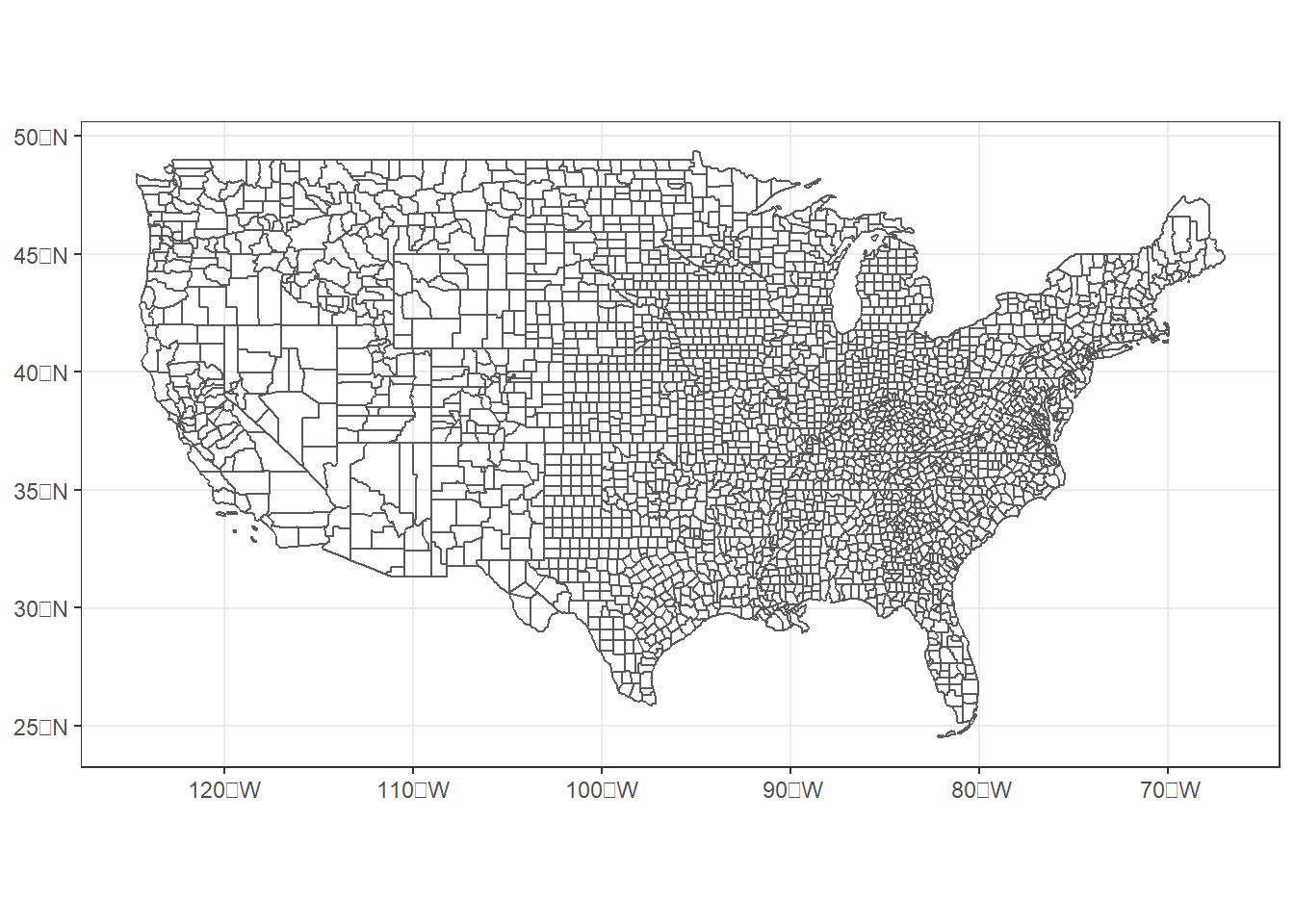

FIGURE 8.1: U.S. counties mapped in a geographic coordinate system.

The st_crs() function returns a list containing various data elements that describe the projection, and the projection name, EPSG code, PROJ.4 string code, and WKT string code can be viewed by selecting the appropriate list elements. The following code extracts and prints the projection name and EPSG code.

st_crs(county)$Name
## [1] "NAD83"
st_crs(county)$epsg
## [1] 4269

The PROJ.4 format, stored in the proj4string element, is an older, abbreviated format for storing CRS parameters. This format is no longer recommended for defining coordinate systems in R because of changes in the underlying RPROJ software library.

st_crs(county)$proj4string
## [1] "+proj=longlat +datum=NAD83 +no_defs"

Well-known text (WKT) is a more comprehensive format that is currently recommended for defining and storing CRS information in R. However, WKT can be difficult for humans to read. Extracting the WktPretty element and printing it to the console using the writeLines() function provide a formatted version of the WKT string that makes it easier to see the various CRS parameters.

writeLines(st_crs(county)$WktPretty)
## GEOGCS["NAD83",
##     DATUM["North_American_Datum_1983",
##         SPHEROID["GRS 1980",6378137,298.257222101]],
##     PRIMEM["Greenwich",0],
##     UNIT["degree",0.0174532925199433,
##         AUTHORITY["EPSG","9122"]],
##     AXIS["Latitude",NORTH],
##     AXIS["Longitude",EAST],
##     AUTHORITY["EPSG","4269"]]

The st_transform() function is used to reproject sf objects. The first argument is the spatial dataset to reproject. The second argument is the coordinate system into which the data will be reprojected. The coordinate system information can be entered in several different ways. Here, we simply enter another EPSG code (5070) which is a commonly-used Albers Equal Area projection for the conterminous United States.

county_aea <- st_transform(county, 5070)
writeLines(st_crs(county_aea)$WktPretty)
## PROJCS["NAD83 / Conus Albers",
##     GEOGCS["NAD83",
##         DATUM["North_American_Datum_1983",
##             SPHEROID["GRS 1980",6378137,298.257222101]],
##         PRIMEM["Greenwich",0],
##         UNIT["degree",0.0174532925199433,
##             AUTHORITY["EPSG","9122"]],
##         AUTHORITY["EPSG","4269"]],
##     PROJECTION["Albers_Conic_Equal_Area"],
##     PARAMETER["latitude_of_center",23],
##     PARAMETER["longitude_of_center",-96],
##     PARAMETER["standard_parallel_1",29.5],
##     PARAMETER["standard_parallel_2",45.5],
##     PARAMETER["false_easting",0],
##     PARAMETER["false_northing",0],
##     UNIT["metre",1],
##     AXIS["Easting",EAST],
##     AXIS["Northing",NORTH],
##     AUTHORITY["EPSG","5070"]]

In the resulting map, note that the x and y axes of the coordinate system no longer correspond to the graticules of latitude and longitude (Figure 8.2).

ggplot(data = county_aea) +
  geom_sf(fill = NA) +
  theme_bw()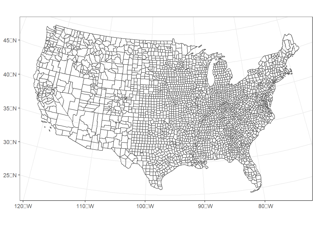

FIGURE 8.2: U.S. counties projected into an Albers Equal Area coordinate system for the conterminous United States.

Using EPSG codes is the recommended method for specifying coordinate systems because specifying these codes is much simpler than entering all the underlying projection details. The following websites can be used to look up EPSG codes for different coordinate reference systems.

Another way to define the projection is to enter all of the projection details directly using the well-known text (WKT version 2) projection format. This approach requires the user to provide a string containing the specification and parameters of the datum and coordinate system. This example specifies a “bad” projection that is based on the Albers projection for the conterminous United States. In this example, the standard parallels have been shifted northward to the Arctic Circle, which should result in considerable distortion.

badcrs_wkt <- 
'PROJCS["BadAlbers",
GEOGCS["NAD83",
  DATUM["North_American_Datum_1983",
    SPHEROID["GRS 1980",6378137,298.257222101]],
  PRIMEM["Greenwich",0],
  UNIT["degree",0.0174532925199433]],
PROJECTION["Albers_Conic_Equal_Area"],
PARAMETER["latitude_of_center",37.5],
PARAMETER["longitude_of_center",-96],
PARAMETER["standard_parallel_1",75],
PARAMETER["standard_parallel_2",80],
PARAMETER["false_easting",0],
PARAMETER["false_northing",0],
UNIT["metre",1],
AXIS["Easting",EAST],
AXIS["Northing",NORTH]]'

mybadcrs <- st_crs(badcrs_wkt)
county_bad <- st_transform(county, mybadcrs)

The resulting map does not look very good. There is unnecessary distortion because the standard parallels are outside of the area being mapped (Figure 8.3).

ggplot(data = county_bad) +
  geom_sf(fill = NA) +
  theme_bw()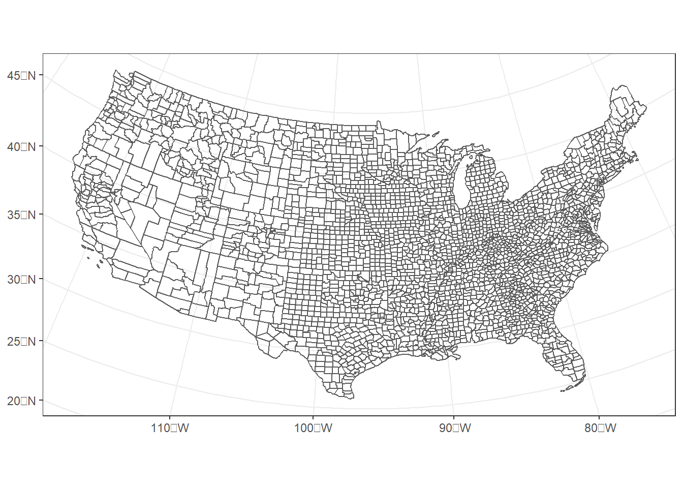

FIGURE 8.3: U.S. counties projected into an Albers Equal Area coordinate system with standard parallels located too far north.

Often, the most straightforward way to specify a CRS is to use the information from another geospatial datasets that is in the desired CRS. An easy way to do this is to use the st_crs() function to extract the coordinate reference system from the other spatial dataset. Here, we reproject the county dataset with the “bad” projection back to the Albers Equal Area projection from the county_aea dataset (Figure 8.4).

county_fixed <- st_transform(county_bad, st_crs(county_aea))
ggplot(data = county_fixed) +
  geom_sf(fill = NA) +
  theme_bw()

FIGURE 8.4: U.S. counties projected back to an Albers Equal Area coordinate system for the conterminous United States.

This approach is a straightforward way to make sure all the data are in the same projection. Start by projecting one of your datasets into the desired coordinate system and then project all the other datasets to match this baseline dataset.

Here are a few more examples looking at just the state of New York. It looks a bit tilted because it is at the edge of the conterminous U.S. and thus gets distorted by the national-level Albers projection (Figure 8.5).

newyork <- filter(county_aea, state == 36)
ggplot(data = newyork) +
  geom_sf(fill = NA) +
  theme_bw()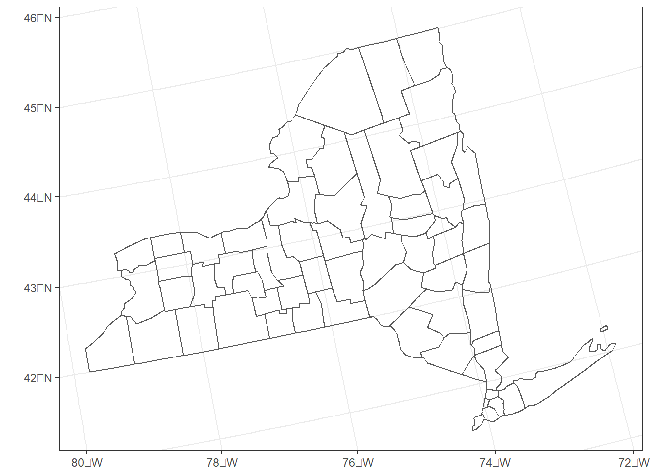

FIGURE 8.5: New York counties in an Albers Equal Area coordinate system for the conterminous United States.

It can be made to look a bit better by putting it in a more localized UTM projection, Universal Transverse Mercator (UTM) zone 18 north. In this case, the EPSG code of 26918 represents UTM zone 18 north with a NAD83 datum (Figure 8.6).

ny_utm <- st_transform(newyork, 26918)
writeLines(st_crs(ny_utm)$WktPretty)
## PROJCS["NAD83 / UTM zone 18N",
##     GEOGCS["NAD83",
##         DATUM["North_American_Datum_1983",
##             SPHEROID["GRS 1980",6378137,298.257222101]],
##         PRIMEM["Greenwich",0],
##         UNIT["degree",0.0174532925199433,
##             AUTHORITY["EPSG","9122"]],
##         AUTHORITY["EPSG","4269"]],
##     PROJECTION["Transverse_Mercator"],
##     PARAMETER["latitude_of_origin",0],
##     PARAMETER["central_meridian",-75],
##     PARAMETER["scale_factor",0.9996],
##     PARAMETER["false_easting",500000],
##     PARAMETER["false_northing",0],
##     UNIT["metre",1],
##     AXIS["Easting",EAST],
##     AXIS["Northing",NORTH],
##     AUTHORITY["EPSG","26918"]]

ggplot(data = ny_utm) +
  geom_sf(fill = NA) +
  theme_bw()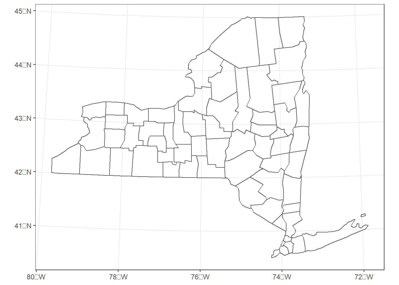

FIGURE 8.6: New York counties in the UTM zone 18 north coordinate system.

8.2 Reprojecting Raster Data

Here, we will take another look at the Walton County raster dataset that was used in Chapter 7. The raster grid is 1579 rows by 1809 columns, and each cell is a 30 m square.

landcov <- rast("NLCD_2016_Land_Cover_Walton.tiff")
nrow(landcov)
## [1] 1579
ncol(landcov)
## [1] 1809
res(landcov)
## [1] 30 30
ext(landcov)[1:4]
##    xmin    xmax    ymin    ymax 
## 1096815 1151085 1237395 1284765

The terra function crs() returns detailed projection information for SpatRaster objects. The writeLines() function parses the projection parameters and writes them to the console in a more readable format. These data have a similar Albers Equal Area projection to the one used for the county data.

writeLines(crs(landcov))
## PROJCRS["Albers_Conical_Equal_Area",
##     BASEGEOGCRS["NAD83",
##         DATUM["North American Datum 1983",
##             ELLIPSOID["GRS 1980",6378137,298.257222101004,
##                 LENGTHUNIT["metre",1]]],
##         PRIMEM["Greenwich",0,
##             ANGLEUNIT["degree",0.0174532925199433]],
##         ID["EPSG",4269]],
##     CONVERSION["Albers Equal Area",
##         METHOD["Albers Equal Area",
##             ID["EPSG",9822]],
##         PARAMETER["Latitude of false origin",23,
##             ANGLEUNIT["degree",0.0174532925199433],
##             ID["EPSG",8821]],
##         PARAMETER["Longitude of false origin",-96,
##             ANGLEUNIT["degree",0.0174532925199433],
##             ID["EPSG",8822]],
##         PARAMETER["Latitude of 1st standard parallel",29.5,
##             ANGLEUNIT["degree",0.0174532925199433],
##             ID["EPSG",8823]],
##         PARAMETER["Latitude of 2nd standard parallel",45.5,
##             ANGLEUNIT["degree",0.0174532925199433],
##             ID["EPSG",8824]],
##         PARAMETER["Easting at false origin",0,
##             LENGTHUNIT["metre",1],
##             ID["EPSG",8826]],
##         PARAMETER["Northing at false origin",0,
##             LENGTHUNIT["metre",1],
##             ID["EPSG",8827]]],
##     CS[Cartesian,2],
##         AXIS["easting",east,
##             ORDER[1],
##             LENGTHUNIT["metre",1,
##                 ID["EPSG",9001]]],
##         AXIS["northing",north,
##             ORDER[2],
##             LENGTHUNIT["metre",1,
##                 ID["EPSG",9001]]]]

To see only the projection name, use the describe = TRUE argument with crs() and extract the name element from the data frame that is returned.

crs(landcov, describe = TRUE)$name
## [1] "Albers_Conical_Equal_Area"

The st_crs() function from the sf package can also be used to extract CRS information from spatRaster objects. This approach prints the CRS in a format that is a bit more compact and easy to read than the output of the crs() function.

writeLines(st_crs(landcov)$WktPretty)
## PROJCS["Albers_Conical_Equal_Area",
##     GEOGCS["NAD83",
##         DATUM["North_American_Datum_1983",
##             SPHEROID["GRS 1980",6378137,298.257222101004]],
##         PRIMEM["Greenwich",0],
##         UNIT["degree",0.0174532925199433,
##             AUTHORITY["EPSG","9122"]],
##         AUTHORITY["EPSG","4269"]],
##     PROJECTION["Albers_Conic_Equal_Area"],
##     PARAMETER["latitude_of_center",23],
##     PARAMETER["longitude_of_center",-96],
##     PARAMETER["standard_parallel_1",29.5],
##     PARAMETER["standard_parallel_2",45.5],
##     PARAMETER["false_easting",0],
##     PARAMETER["false_northing",0],
##     UNIT["metre",1,
##         AUTHORITY["EPSG","9001"]],
##     AXIS["Easting",EAST],
##     AXIS["Northing",NORTH]]

Before mapping the land cover data, they are reclassified into seven broader classes as in Chapter 7.

oldclas <- unique(landcov)
newclas <- c(1, 2, 2, 2, 2, 3, 4, 4, 4, 5, 5, 5, 6, 7, 7)
lookup <- data.frame(oldclas, newclas)
landcov_rc <- classify(landcov, lookup)
newnames <- c("Water",
               "Developed",
               "Barren",
               "Forest",
               "GrassShrub",
               "Cropland",
               "Wetland")
newcols <- c("mediumblue", 
             "red2", 
             "gray60", 
             "darkgreen", 
             "yellow2", 
             "orange4", 
             "paleturquoise2")
newcols2 <- desaturate(newcols, amount = 0.3)

The data are then converted to a data frame using the rasterdf() function and mapped (Figure 8.7).

source("rasterdf.R")
landcov_df <- rasterdf(landcov_rc)

ggplot(data = landcov_df) +
  geom_raster(aes(x = x, 
                  y = y, 
                  fill = as.character(value))) + 
  scale_fill_manual(name = "Land cover",
                    values = newcols2,
                    labels = newnames,
                    na.translate = FALSE) +
  coord_sf(expand = FALSE) +
  theme_void()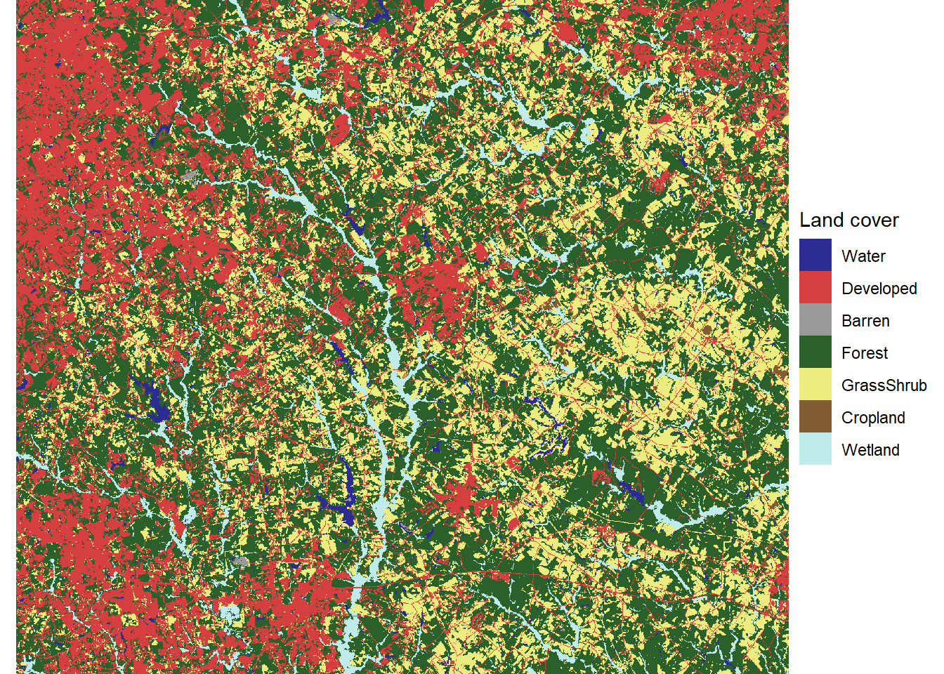

FIGURE 8.7: Walton County land cover data in an Albers Equal Area coordinate reference system for the conterminous United States.

These data will be projected into a UTM projection (zone 17 north) and NAD 83 datum using an EPSG code (26917) as was done for the New York dataset. Raster data are reprojected using the project() function from the terra package. When raster data are reprojected, the values must be resampled onto a new raster grid in the updated projection. Like the st_transform() function, the first argument is the dataset to be reprojected, and the second argument is the new CRS. Note that the format for specifying EPSG codes is a bit different when working with rasters in the terra package. Instead of just a number, a string must be provided with epsg: preceding the number.

By default, the project() function uses bilinear interpolation, which is appropriate for continuous data such as elevation or temperature. For land cover data, interpolated values that fall in between the numerical class codes would be meaningless. Therefore, the argument method = "near" must be specified to use nearest neighbor interpolation, which preserves the class codes. For continuous data, this argument can be omitted or method = "bilinear" can be explicitly used. Specifying res = 30 ensures that the output raster has the same cell size (30 m) as the input raster.

landcov_utm <- project(landcov_rc, "epsg:26917", 
                       method = "near",
                       res = 30)
crs(landcov_utm, describe = TRUE)$name
## [1] "NAD83 / UTM zone 17N"

The coordinate reference system has been changed, and the numbers of rows and columns in the raster have increased as well.

nrow(landcov_utm)
## [1] 1828
ncol(landcov_utm)
## [1] 2047
res(landcov_utm)
## [1] 30 30

These changes are apparent in the map of the reprojected Walton County data (Figure 8.8). As was observed with New York State, the orientation of the dataset has shifted after projecting into UTM. Because raster layers must be rectangular grids, the overall size of the raster is increased to accomodate the new orientation of the dataset, and NA values are used to account for cells in the new raster that are outside of the boundaries of the original dataset.

landcovutm_df <- rasterdf(landcov_utm)
ggplot(data = landcovutm_df) +
  geom_raster(aes(x = x, 
                  y = y, 
                  fill = as.character(value))) + 
  scale_fill_manual(name = "Land cover",
                    values = newcols2,
                    labels = newnames,
                    na.translate = FALSE) +
  coord_sf(expand = FALSE) +
  theme_void()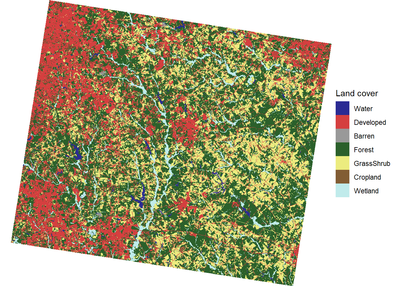

FIGURE 8.8: Walton County land cover data in Universal Transverse Mercator coordinate system.

As with vector data, a simple way to reproject raster data is to specify a raster dataset from which to obtain information about the desired CRS, cell size, grid size, and grid origin. In this example, the Walton County data are reprojected from UTM back to the original Albers Equal Area coordinate system. The first argument to the project() function is the raster dataset to be projected, and the second argument is another raster dataset that provides the CRS and raster grid information.

landcov_goback <- project(landcov_utm, 
                          landcov, 
                          method = "near")

Now the landcov_goback dataset has the same projection as the original landcov dataset. The compareGeom() function can be used to confirm that the two rasters have the exact same geometry, with identical extents, numbers of rows and columns, coordinate reference systems, cell sizes, and origins.

crs(landcov_goback, describe = TRUE)$name
## [1] "Albers_Conical_Equal_Area"
crs(landcov_rc, describe = TRUE)$name
## [1] "Albers_Conical_Equal_Area"
compareGeom(landcov_rc, landcov_goback)
## [1] TRUE

The landcov and landcov_goback rasters have the same geometry, but what about the actual data? Here, the freq() function is used here to compare the number of cells in each land cover class to see if projecting into UTM and then back to the original Albers Equal Area coordinate system has altered the data.

freq(landcov_rc)
##      layer value   count
## [1,]     1     1   37165
## [2,]     1     2  687865
## [3,]     1     3    7928
## [4,]     1     4 1296342
## [5,]     1     5  691107
## [6,]     1     6    6629
## [7,]     1     7  129375
freq(landcov_goback)
##      layer value   count
## [1,]     1     1   37182
## [2,]     1     2  687909
## [3,]     1     3    7916
## [4,]     1     4 1296069
## [5,]     1     5  691183
## [6,]     1     6    6631
## [7,]     1     7  129411

It appears that the distributions of land cover types do not match exactly. To look at the changes more closely, the crosstab() function is applied in a similar manner to the way it was used to generate change matrices in Chapter 7. Here, instead of looking at change over time, the crosstabulation quantifies differences between landcov_rc and landcov_goback .

projcomp <- crosstab(c(landcov_rc, landcov_goback))
shortnames <- c("Wat", 
                "Dev", 
                "Bare", 
                "For", 
                "Grass", 
                "Crop", 
                "Wet")
rownames(projcomp) <- shortnames
colnames(projcomp) <- shortnames

When examining the crosstabulation, the numbers along the diagonal from upper left to lower right are counts of cells that have the same land cover code in both datasets (8.1). Numbers in the upper right and lower left off-diagonal triangles indicate cells that have different values in the landcov_rc and landcov_goback datasets. It is clear from these results that while most of the cell values are the same in both datasets, reprojecting the landcov_goback dataset twice has altered the land cover codes in some of the cells.

TABLE 8.1: Crosstabulation of cell values from the original Walton County land cover dataset (rows) and the same data projected into UTM and then back to the original Albers Equal Area CRS.
	Wat	Dev	Bare	For	Grass	Crop	Wet
Wat	36508	72	7	377	157	0	43
Dev	61	678023	76	5156	4370	14	137
Bare	7	70	7678	57	113	0	3
For	408	5299	59	1284073	5101	5	1348
Grass	166	4297	93	5081	681232	44	164
Crop	0	10	1	6	44	6567	1
Wet	32	138	2	1319	166	1	127715

This is an important point when working with raster data. Reprojecting rasters always changes the data because they have to be resampled to a new grid in the new coordinate system. This process alters the distribution of cell-level data values and is not exactly reversible. The bottom line is to avoid reprojecting raster datasets more than once. Instead, go back to the original data and reproject from the native coordinate system if you can. When combining raster and vector data, avoid reprojecting the rasters if possible and instead reproject the vector data to match the CRS of the rasters.

8.3 Specifying Coordinate Reference Systems

All spatial data must use some type of coordinate reference system to specify locations. However, in some cases, a spatial dataset may lack information about its coordinate reference system. For example, the PRJ file of a shapefile may get lost when copying the data from one location to another. In this case, it is often necessary to do some detective work to determine the actual coordinate reference system and then specify it after the data have been imported into R. This example reads in another version of the U.S. county shapefile where the PRJ file has been deleted.

county_nocrs <- st_read("cb_2018_us_county_noPRJ.shp", quiet = TRUE)
county_nocrs <- county_nocrs %>%
  mutate(state = as.numeric(as.character(STATEFP))) %>%
  filter(state != 2, state != 15, state < 60)

These data can still be mapped (Figure 8.9), but the software does not know whether the coordinates represent latitude and longitude or some type of distance units relative to the origin of a projected CRS. This is similar to a situation where there is a dataset with nonspatial measurements such as tree heights, but the units of measurement have not been recorded. We cannot make use of the tree heights until we find out if they are in centimeters, inches, feet, or meters. Similarly, geospatial data cannot be used effectively without knowledge of the underlying CRS.

st_crs(county_nocrs)
## Coordinate Reference System: NA
ggplot(data = county_nocrs) +
  geom_sf(fill = NA) +
  theme_bw()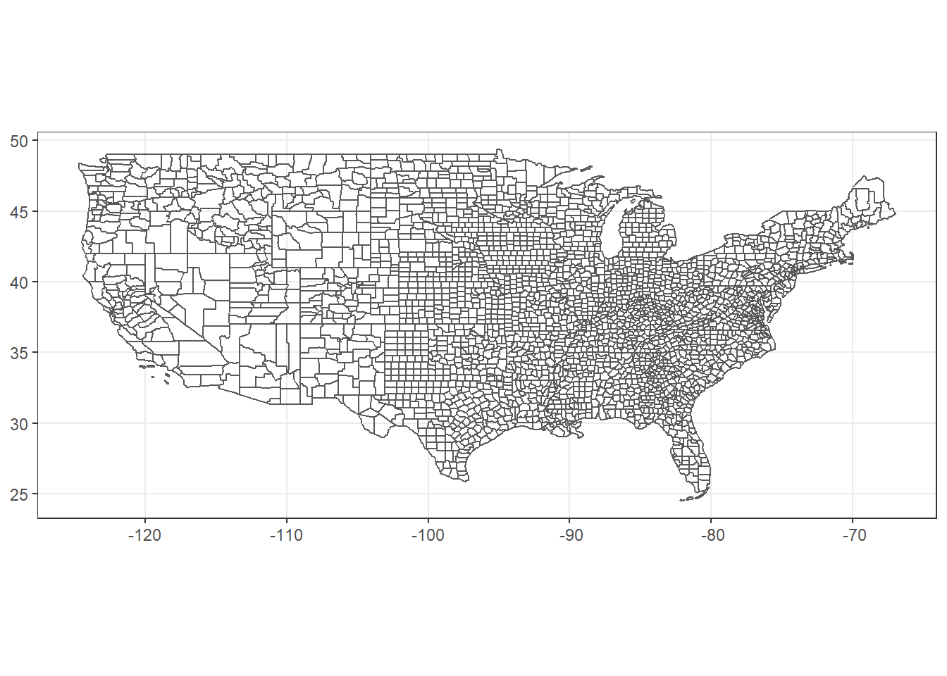

FIGURE 8.9: U.S. counties mapped in a geographic coordinate system using a dataset that is missing CRS information.

If the current CRS is not defined, it is not possible to reproject the data into a new CRS. Attemping to use the st_transform() function with the county_nocrs data will return an error. Referring back to the tree height example, we cannot convert tree heights with unkown units to meters until we known if the current units are centimeters, inches, or feet, or perhaps they are already in meters.

county_newcrs <- st_transform(county_nocrs, 4269)

Although, the coordinate system is undefined, a look at the map clearly shows that the data have geographic coordinates (Figure 8.9). This is apparent from the range of coordinate values as well as the characteristic distortion that we see when angular coordinates are plotted on a two-dimensional map. The problem is that the necessary metadata to identify the coordinate system is not present. To specify a missing coordinate system, the st_set_crs() function is used with the EPSG code for geographic coordinates in a NAD83 datum (4269).

county_crs <- st_set_crs(county_nocrs, 4269)
writeLines(st_crs(county_crs)$WktPretty)
## GEOGCS["NAD83",
##     DATUM["North_American_Datum_1983",
##         SPHEROID["GRS 1980",6378137,298.257222101]],
##     PRIMEM["Greenwich",0],
##     UNIT["degree",0.0174532925199433,
##         AUTHORITY["EPSG","9122"]],
##     AXIS["Latitude",NORTH],
##     AXIS["Longitude",EAST],
##     AUTHORITY["EPSG","4269"]]

Now that the proper coordinate reference system has been assigned, it is possible to project the data into another CRS.

county_newcrs <- st_transform(county_crs, 5070)
writeLines(st_crs(county_newcrs)$WktPretty)
## PROJCS["NAD83 / Conus Albers",
##     GEOGCS["NAD83",
##         DATUM["North_American_Datum_1983",
##             SPHEROID["GRS 1980",6378137,298.257222101]],
##         PRIMEM["Greenwich",0],
##         UNIT["degree",0.0174532925199433,
##             AUTHORITY["EPSG","9122"]],
##         AUTHORITY["EPSG","4269"]],
##     PROJECTION["Albers_Conic_Equal_Area"],
##     PARAMETER["latitude_of_center",23],
##     PARAMETER["longitude_of_center",-96],
##     PARAMETER["standard_parallel_1",29.5],
##     PARAMETER["standard_parallel_2",45.5],
##     PARAMETER["false_easting",0],
##     PARAMETER["false_northing",0],
##     UNIT["metre",1],
##     AXIS["Easting",EAST],
##     AXIS["Northing",NORTH],
##     AUTHORITY["EPSG","5070"]]

It is also possible to assign coordinate reference systems to raster data using the crs() function in the terra() package. For example, if myraster_nocrs is a raster datasets with no CRS specified, it can be assigned a coordinate system by specifying an EPSG code or assigning the CRS from another raster dataset.

crs(raster_nocrs) <- "epsg:4326"
crs(raster_nocrs) <- crs(raster_withcrs)

This chapter has provided a very basic introduction to working with coordinate references systems in R, with a focus on just a few examples from North America. For more background on the topic, the book GIS Fundamentals (Bolstad 2019) is an excellent reference. Geocomputation with R (Lovelace, Nowosad, and Muenchow 2019) also contains a chapter on reprojecting geographic data in R.

8.4 Practice

Generate an sf object for the state of California (state FIPS code = 6). Compare maps of the state in a geographic projection (EPSG code 4269), Albers equal area projection (EPSG code 5070), and UTM zones 10 and 11 (EPSG codes 26910 and 26911). Explore how the different coordinate reference systems affect the shape and orientation of the state.
Reproject the Walton County land cover dataset into the same geographic coordinate system used in the U.S. county dataset. Specify a resolution of 0.008333 degrees (30 arc seconds) for the reprojected raster.