Chapter 4 Dates in R

Several examples that use Date objects have already been shown in the preceding chapters. Dates are important in geographical data science because most environmental measurements are repeated over time. For example, automated weather stations can collect meteorological data on hourly or shorter measurement cycles, and Earth-observing satellites acquire images at a given location on daily to weekly cycles. These repeated measurements provide the basis for analyzing environmental change. When working with these data in R, it is essential to have information about the timing of observations as well as their locations in geographic space. This chapter will provide an overview of how to work with dates in R using the lubridate package (Spinu, Grolemund, and Wickham 2021).

library(ggplot2)
library(dplyr)
library(readr)
library(lubridate)

4.1 Converting Characters to Dates

The testdates.csv file contains daily temperature measurements from an Oklahoma Mesonet station. The date of each observation is provided in a variety of formats, and these variables will be used to learn about manipulating dates with lubridate. Figure 4.1 shows the formats of the raw data in testdates.csv. The first row contains the column names, and the subsequent rows contain the data with each variable separated by a comma.

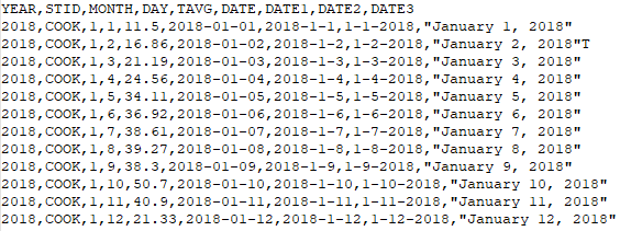
FIGURE 4.1: Contents of the testdates.csv file.

The columns contain the following information.

YEAR: Year of meteorological observation
STID: Meteorological station ID code
MONTH: Month of meteorological observation
DAY: Day of month of meteorological observation
TAVG: Average temperature for date of observation
DATE: Date formatted as “2018-01-09” (YYYY-MM-DD with leading zeroes)
DATE1: Date formatted as “2018-1-9” (YYYY-MM-DD with no leading zeroes)
DATE2: Date formatted as “1-9-2018” (MM-DD-YYYY with no leading zeroes)
DATE3: Date formatted as “January 9, 2018” (MONTHNAME, DD, YYYY with no leading zeroes)

datefile <- read_csv("testdates.csv", show_col_type = FALSE)
glimpse(datefile)
## Rows: 365
## Columns: 9
## $ YEAR  <dbl> 2018, 2018, 2018, 2018, 2018, 2018, 2018, 20…
## $ STID  <chr> "COOK", "COOK", "COOK", "COOK", "COOK", "COO…
## $ MONTH <dbl> 1, 1, 1, 1, 1, 1, 1, 1, 1, 1, 1, 1, 1, 1, 1,…
## $ DAY   <dbl> 1, 2, 3, 4, 5, 6, 7, 8, 9, 10, 11, 12, 13, 1…
## $ TAVG  <dbl> 11.50, 16.86, 21.19, 24.56, 34.11, 36.92, 38…
## $ DATE  <date> 2018-01-01, 2018-01-02, 2018-01-03, 2018-01…
## $ DATE1 <chr> "2018-1-1", "2018-1-2", "2018-1-3", "2018-1-…
## $ DATE2 <chr> "1-1-2018", "1-2-2018", "1-3-2018", "1-4-201…
## $ DATE3 <chr> "January 1, 2018", "January 2, 2018", "Janua…

Note that read_csv() correctly interprets the DATE column and converts it to a Date object in R. The other date formats remain as character strings. The DATE column contains values formatted as YYYY-MM-DD. For example, January 1, 2018 is specified as 2018-01-01. There are always two digits for the month and day of the month, with leading zeroes included when these values are less than ten. The read_csv() function is able to recognize this format and automatically convert it to a date. The DATE1 and DATE2 columns are specified as YYYY-MM-DD and MM-DD-YYYY, and these columns do not include leading zeroes. Because these formats are more ambiguous, the dates cannot be automatically interpreted, and these columns are read as character strings. The same is true for the DATE3 column that spells out the month name.

Environmental datasets use a wide variety of date formats. Years, months, and days can be arranged in different orders using different separators. Months may be spelled out or numbered. Single-digit months and days may or may not have leading zeroes. In some cases, the month and day of the month may be replaced by a single number representing the day of the year.

These differences are especially problematic when data must be imported from multiple sources and joined by date. Furthermore, it is not uncommon to find inconsistently formatted date strings within a single dataset. Variables representing dates should always be carefully screened when importing a dataset, and extra attention is warranted to ensure that code is written to process the date variables correctly.

A Date object in R is stored as an integer value that represents the number of days before or after the baseline date of January 1, 1970. The following example generates a vector of date objects and shows their corresponding numeric values.

mydates <- as.Date(c("1932-01-01", "1950-12-25", "1968-04-28",
                   "1990-06-24", "2003-07-04", "2033-11-15"))
as.numeric(mydates)
## [1] -13880  -6947   -613   7479  12237  23329

Other operators and functions in R are able to recognize the Date class, and they can extract and manipulate other types of information (years, months, weeks, days) associated with dates. For example, if we plot the DATE column on the x-axis of a graph, ggplot() knows how to handle it, and we get a time series plot of temperature (Figure 4.2). Tick marks on the x-axis are referenced by month and year.

ggplot(data = datefile) +
  geom_line(aes(x = DATE, y = TAVG)) +
  labs(x = "Correct Date", 
       y = "Temperature (\u00B0F)")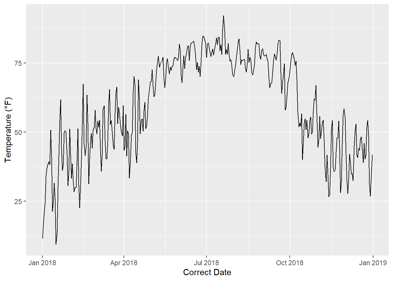

FIGURE 4.2: Time series plot with dates on the x-axis.

The DATE1, DATE2, and DATE3 columns all contain dates stored as character objects. If we tried to use one of these columns to make a time series graph in ggplot(), it would be interpreted a categorical variable instead of a continuous time variable. Fortunately, it is relatively easy to convert character strings into dates. Base R has an as.Date() function that can convert some types of strings into Date objects.

datefile <- datefile %>%
  mutate(DATE1B = as.Date(DATE1),
         DATE2B = as.Date(DATE2))
glimpse(datefile)
## Rows: 365
## Columns: 11
## $ YEAR   <dbl> 2018, 2018, 2018, 2018, 2018, 2018, 2018, 2…
## $ STID   <chr> "COOK", "COOK", "COOK", "COOK", "COOK", "CO…
## $ MONTH  <dbl> 1, 1, 1, 1, 1, 1, 1, 1, 1, 1, 1, 1, 1, 1, 1…
## $ DAY    <dbl> 1, 2, 3, 4, 5, 6, 7, 8, 9, 10, 11, 12, 13, …
## $ TAVG   <dbl> 11.50, 16.86, 21.19, 24.56, 34.11, 36.92, 3…
## $ DATE   <date> 2018-01-01, 2018-01-02, 2018-01-03, 2018-0…
## $ DATE1  <chr> "2018-1-1", "2018-1-2", "2018-1-3", "2018-1…
## $ DATE2  <chr> "1-1-2018", "1-2-2018", "1-3-2018", "1-4-20…
## $ DATE3  <chr> "January 1, 2018", "January 2, 2018", "Janu…
## $ DATE1B <date> 2018-01-01, 2018-01-02, 2018-01-03, 2018-0…
## $ DATE2B <date> 0001-01-20, 0001-02-20, 0001-03-20, 0001-0…

The new DATE1B and DATE2B columns contain date objects. However, if we tried to convert the DATE3 column, R would return an error because as.Date() is not able to recognize the month names or the comma and space separators.

The conversion from character in DATE1 to Date in DATE1B is successful, and a valid time series plot can be generated using DATE1B (Figure 4.3).

ggplot(data = datefile) +
  geom_line(aes(x = DATE1B, y = TAVG)) +
  ggtitle("DATE1 correctly converted to a date with as.Date()")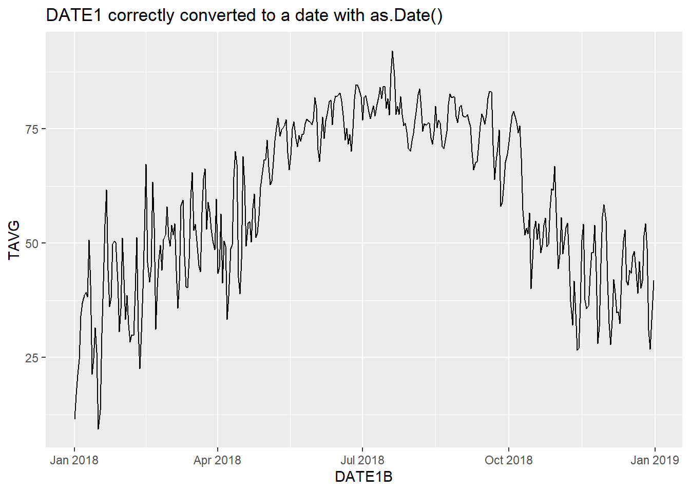

FIGURE 4.3: Time series plot with dates successfully converted using as.Date().

The conversion of DATE2, which is in MM-DD-YYYY format instead of YYYY-MM-DD format, produces a valid Date object in column DATE2B. However, by default, the as.Date() function assumes that the date string is in Year-Day-Month format, dates in the MM-DD-YYYY format are either read incorrectly or assigned a value of NA. The resulting time series graph shows dates from a range of years at the beginning of the Common Era (Figure 4.4). These are clearly the wrong dates for the 2018 weather dataset.

ggplot(data = datefile) +
  geom_line(aes(x = DATE2B, y = TAVG)) +
  ggtitle("DATE2 incorrectly converted to a date with as.Date()")
## Warning: Removed 221 row(s) containing missing values
## (geom_path).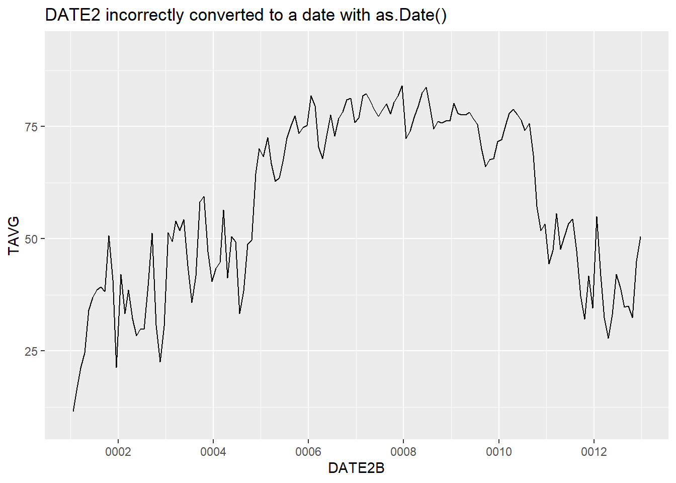

FIGURE 4.4: Time series plot with dates unsuccessfully converted using as.Date().

To convert DATE2 to a date object using as.Date(), additional information about the formatting of the date string must be provided as a function argument. This can be done for specifying an additional string with formatting codes. An alternative is to use a package with functions that simplify the creation and manipulation of Date objects. This book uses lubridate, another member of the tidyverse collection of packages.

In the following example, the ymd() function from lubridate is used to transform character strings in YYYY-MM-DD format into date objects, and the mdy() function is used to transform the MM-DD-YYYY format.

datefile <- datefile %>%
  mutate(DATE1C = ymd(DATE1),
         DATE2C = mdy(DATE2),
         DATE3C = mdy(DATE3))
glimpse(datefile)
## Rows: 365
## Columns: 14
## $ YEAR   <dbl> 2018, 2018, 2018, 2018, 2018, 2018, 2018, 2…
## $ STID   <chr> "COOK", "COOK", "COOK", "COOK", "COOK", "CO…
## $ MONTH  <dbl> 1, 1, 1, 1, 1, 1, 1, 1, 1, 1, 1, 1, 1, 1, 1…
## $ DAY    <dbl> 1, 2, 3, 4, 5, 6, 7, 8, 9, 10, 11, 12, 13, …
## $ TAVG   <dbl> 11.50, 16.86, 21.19, 24.56, 34.11, 36.92, 3…
## $ DATE   <date> 2018-01-01, 2018-01-02, 2018-01-03, 2018-0…
## $ DATE1  <chr> "2018-1-1", "2018-1-2", "2018-1-3", "2018-1…
## $ DATE2  <chr> "1-1-2018", "1-2-2018", "1-3-2018", "1-4-20…
## $ DATE3  <chr> "January 1, 2018", "January 2, 2018", "Janu…
## $ DATE1B <date> 2018-01-01, 2018-01-02, 2018-01-03, 2018-0…
## $ DATE2B <date> 0001-01-20, 0001-02-20, 0001-03-20, 0001-0…
## $ DATE1C <date> 2018-01-01, 2018-01-02, 2018-01-03, 2018-0…
## $ DATE2C <date> 2018-01-01, 2018-01-02, 2018-01-03, 2018-0…
## $ DATE3C <date> 2018-01-01, 2018-01-02, 2018-01-03, 2018-0…

The DATE1C, DATE2C, and DATE3C columns all contain the correct dates now.

A handy feature of the lubridate functions is that they are very smart about interpreting in a variety of date formats without the user having to provide explicit formatting information. They can read dates parsed with dashes, slashes, or spaces, and they can deal with months and days with and without leading zeros. They can also deal with other types of date formats, such as the month names in the DATE3 column.

4.2 Other lubridate Operators and Functions

It is common to store different date elements, such as year, month, and day, in different database columns. This is a very effective way of representing date information in a database, since the date components can be stored as simple integers, and the meanings of the values in the year, month, and day columns are unambiguous.

The lubridate functions can be used to combine data from multiple columns into a single date object. A straightforward way to do this is to first use the paste() function to combine multiple values into a date string and then pass the string to the appropriate lubridate function. Here, the variables in the YEAR, MONTH, and DAY columns are combined to create the DAY4 column.

datefile <- datefile %>%
  mutate(DATE4 =ymd(paste(YEAR, MONTH, DAY, sep="-")))
glimpse(datefile)
## Rows: 365
## Columns: 15
## $ YEAR   <dbl> 2018, 2018, 2018, 2018, 2018, 2018, 2018, 2…
## $ STID   <chr> "COOK", "COOK", "COOK", "COOK", "COOK", "CO…
## $ MONTH  <dbl> 1, 1, 1, 1, 1, 1, 1, 1, 1, 1, 1, 1, 1, 1, 1…
## $ DAY    <dbl> 1, 2, 3, 4, 5, 6, 7, 8, 9, 10, 11, 12, 13, …
## $ TAVG   <dbl> 11.50, 16.86, 21.19, 24.56, 34.11, 36.92, 3…
## $ DATE   <date> 2018-01-01, 2018-01-02, 2018-01-03, 2018-0…
## $ DATE1  <chr> "2018-1-1", "2018-1-2", "2018-1-3", "2018-1…
## $ DATE2  <chr> "1-1-2018", "1-2-2018", "1-3-2018", "1-4-20…
## $ DATE3  <chr> "January 1, 2018", "January 2, 2018", "Janu…
## $ DATE1B <date> 2018-01-01, 2018-01-02, 2018-01-03, 2018-0…
## $ DATE2B <date> 0001-01-20, 0001-02-20, 0001-03-20, 0001-0…
## $ DATE1C <date> 2018-01-01, 2018-01-02, 2018-01-03, 2018-0…
## $ DATE2C <date> 2018-01-01, 2018-01-02, 2018-01-03, 2018-0…
## $ DATE3C <date> 2018-01-01, 2018-01-02, 2018-01-03, 2018-0…
## $ DATE4  <date> 2018-01-01, 2018-01-02, 2018-01-03, 2018-0…

Other functions in the lubridate package can be used to extract information from Date objects and to do calculations on them. The following example extracts two dates from the DATE column and stores them as separate objects.

date1 <- datefile$DATE[1]
date2 <- datefile$DATE[180]
date1
## [1] "2018-01-01"
date2
## [1] "2018-06-29"

The examples extract the month, day of the month, year, week of the year, day of the week, and day of the year associated with a Date object. They can be helpful for converting a date object into numbers for storage in separate columns. The day of the year is an important variable when analyzing seasonal patterns of environmental change.

month(date2)
## [1] 6
day(date2)
## [1] 29
year(date2)
## [1] 2018
week(date2)
## [1] 26
wday(date2)
## [1] 6
yday(date2)
## [1] 180

Operators can also be used with date objects. In particular, the - operator is useful for determining the time interval between two dates.

date2 - date1
## Time difference of 179 days
date1 - date2
## Time difference of -179 days

4.3 Practice

Use the code provided below to create two vectors: datetxt contains dates stored as text in month-day-year format, and relhumid contains daily measurements of minimum relative humidity. Convert datetxt to a date object and generate a line graph of changes in relative humidity over time. Create two new vectors that contain the day of the year and the day of the week associated with each observation.

datetxt <- c("3-13-2017", "3-14-2017", "3-15-2017", "3-16-2017",
             "3-17-2017", "3-18-2017", "3-19-2017", "3-20-2017",
             "3-21-2017", "3-22-2017")
relhumid <- c(56, 59, 49, 51, 53, 58, 65, 62, 66, 69)