Chapter 12 Application - Species Distribution Modeling
Climate is one of the most important factors influencing the geographic ranges of species. Each species is adapted to a particular set of climate conditions, which is referred to as its climate niche. The fundamental niche is the hypothetical range of conditions in which a species could persist independently of other species. The realized niche is the narrow range of conditions in which a species can persist when interactions with other species, such as predation and competition, are also taken into account. The realized niche can be characterized by observing where a species is present and absent over large areas and modeling the association between species occurrence and climate variables measured where the species is present and absent (Elith and Leathwick 2009).
Because of the changes in Earth’s climate that are occurring as a result of anthropogenic greenhouse gas emissions, the locations that are most climatically favorable for different species will shift over time. These changes have the potential to radically alter local communities and ecosystems. There is concern that some species may be threatened if they are not able to migrate fast enough to keep up with shifting climate patterns or become disjunct from other mutualistic species such as pollinators. This chapter will explore these issues by modeling the relationships between tree species and climate in mountains of the Pacific Northwest and analyzing how species distributions may change under a future climate change scenario.
Three new packages will be used in this chapter. The spatstat package (Baddeley, Turner, and Rubak 2022) implements methods for the manipulation and analysis of point pattern data. The dismo package (Hijmans et al. 2022) contains a suite of tools for species distribution modeling. The ROCR package (Sing et al. 2005) is used to generate receiver operating characteristics curves and other graphs and statistics to assess prediction accuracy.
library(tidyverse)
library(sf)
library(terra)
library(colorspace)
library(ggspatial)
library(dismo)
library(spatstat)
library(ROCR)
source("rasterdf.R")
12.1 Tree Species Data
The study will encompass the Cascade Mountain Range in Washington State. This area encompasses three ecoregions: the Cascades, East Cascades, and North Cascades. These polygons are read in from a shapefile. Two additional datasets are read in with presence and absence points for subalpine fir (Abies lasiocarpa) and Douglas-fir (Pseudotsuga menziesii). Note that Douglas is a proper name, and Douglas-fir is not a true fir in the genus Abies, which is why the common name of the species is capitalized and hyphenated. The data are from forest inventory plots monitored by the U.S. Forest Service and other land management agencies. These data files were derived from the archived datasets provided by Charney et al. (2021).
wacascades <- st_read("wacascades.shp", quiet = TRUE)
abla <- read_csv("abla.csv")
psme <- read_csv("psme.csv")
The abla and psme data frames contain columns for longitude and latitude (X and Y) along with a column of binary (1/0) data for species presence/absence. These data frames are converted into sf objects and assigned the correct coordinate system (geographic with NAD83 datum).
abla_pts <- st_as_sf(abla,
                     coords = c("X", "Y"))
st_crs(abla_pts) <- 4326
psme_pts <- st_as_sf(psme,
                     coords = c("X", "Y"))
st_crs(psme_pts) <- 4326
The map of presence-absence points shows that subalpine fir is restricted to relatively high elevations near the Cascade crest (Figure 12.1).
ggplot() +
  geom_sf(data = abla_pts,
          aes(color = as.character(abla)),
          size = 0.25) +
  geom_sf(data = wacascades,
          fill = NA) +
  scale_color_manual(name = "Subalpine Fir",
                     values = c("gray", "darkgreen"),
                     labels = c("Absent", "Present")) +
  annotation_scale(location = 'br') +
  theme_void()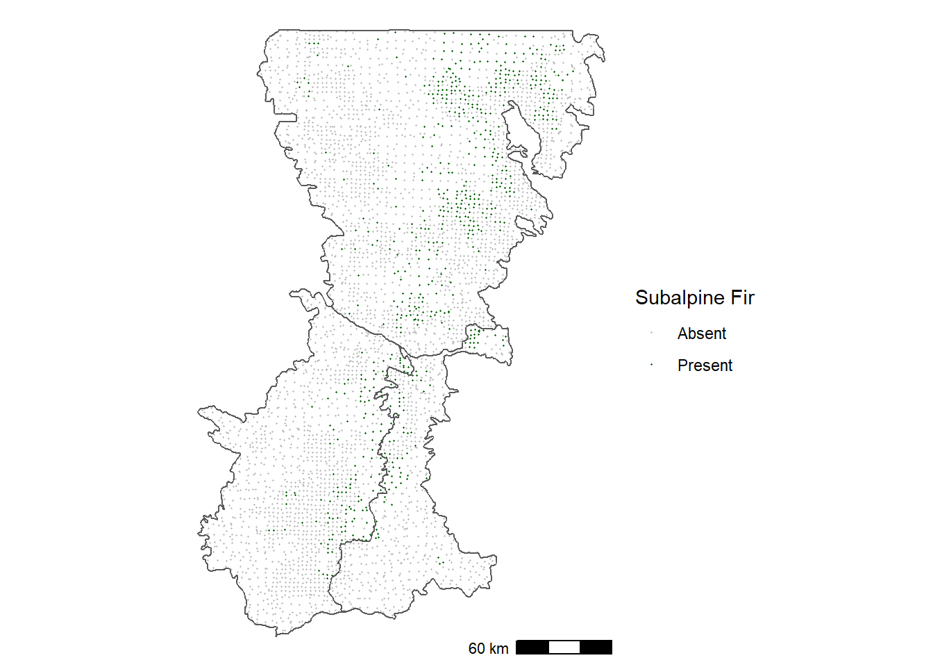
FIGURE 12.1: Occurrence of subalpine fir in forest inventory plots in the Washington Cascades.
In contrast, Douglas-fir is distributed more widely at lower elevations and along the eastern edge of the Cascades (Figure 12.2).
ggplot() +
  geom_sf(data = psme_pts,
          aes(color = as.character(psme)),
          size = 0.25) +
  geom_sf(data = wacascades,
          fill = NA) +
  scale_color_manual(name = "Douglas-fir",
                     values = c("gray", "darkgreen"),
                     labels = c("Absent", "Present")) +
  annotation_scale(location = 'br') +
  theme_void()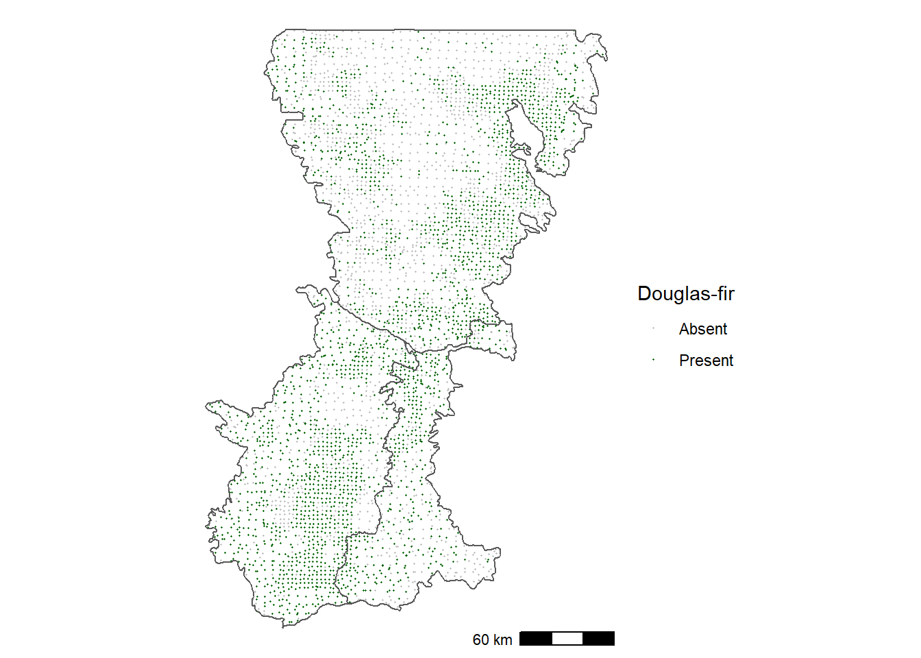
FIGURE 12.2: Occurrence of Douglas-fir in forest inventory plots in the Washington Cascades.
One of the challenges with visualizing the points is that the overall density of plots is variable. In general, there is a higher density of plots on public lands such as National Forests and a lower density on private lands. One way to try to see the occurrence patterns more clearly is to compute kernel-weighted local means. This technique is a type of point-to-raster conversion in which each raster cell in the output is assigned a mean of the local presence/absence values, where points located closer to the cell are given a higher weight than those more distant.
To make this transformation, the point data must be in a projected coordinate system instead of a geographic coordinate system. The Cascades county shapefile as well as the subalpine fir and Dougas-fir point datasets are all reprojected into UTM zone 10 north.
boundary_utm <- st_transform(wacascades, 32610)
abla_utm <- st_transform(abla_pts, 32610)
psme_utm <- st_transform(psme_pts, 32610)
The spatstat package contains a function for generating kernel-weighted means. However, it cannot directly read the data as sf objects. They must first be converted to spatstat ppp objects using the as.ppp() function. The column of ones and zeroes is automatically read in and stored as the “marks” for the point pattern object. Then the as.owin() function is used to create an owin (observation window) object and assign it to the ppp object.
abla_ppp <- as.ppp(abla_utm)
class(abla_ppp)
## [1] "ppp"
Window(abla_ppp) <- as.owin(boundary_utm)
abla_ppp
## Marked planar point pattern: 4356 points
## marks are numeric, of storage type  'double'
## window: polygonal boundary
## enclosing rectangle: [511678.3, 760623.9] x [5046278,
## 5432695] units
The Smooth.ppp() function can now be used to compute kernel-weighted means. The sigma argument specifies the bandwidth of the kernel, which can be conceptualized as the approximate radius of the local window used to compute the means. The eps argument specifies the grid cell size of the output grid. The output is a spatstat im object, which can be converted to a terra SpatRaster object. The coordinate reference system information is lost in the conversion, so the same CRS as the original abla_ppp object is assigned to the new raster dataset.
abla_im <- Smooth.ppp(abla_ppp,
                      sigma=10000,
                      eps=c(1000, 1000))
class(abla_im)
## [1] "im"
abla_grid <- rast(abla_im)
crs(abla_grid) <-"epsg:32610"
The output provides a smoothed estimate of the proportion of plots with subalpine fir (Figure 12.3).
abla_df <- rasterdf(abla_grid)
ggplot(data = abla_df) +
  geom_raster(aes(x = x,
                  y = y,
                  fill = value)) +
  scale_fill_gradient(name = "Subalpine Fir",
                      low = "lightyellow",
                      high = "darkgreen",
                      na.value = NA) +
  geom_sf(data = boundary_utm,
          fill = NA) +
  annotation_scale(location = 'br') +
  coord_sf(expand = F) +
  theme_void()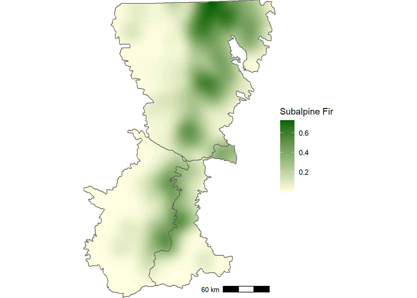
FIGURE 12.3: Smoothed proportion of forest inventory plots with subalpine fir in the Washington Cascades.
The same procedure is repeated for Douglas-fir to generate a smoothed raster of kernel-weighted means.
psme_ppp <- as.ppp(psme_utm)
Window(psme_ppp) <- as.owin(boundary_utm)
psme_im <- Smooth.ppp(psme_ppp,
                      sigma=10000,
                      eps=c(1000, 1000))
psme_grid <- rast(psme_im)
crs(psme_grid) <-"epsg:32610"
Mapping the smoothed occurrence data helps to show that Douglas-fir is broadly distributed in the southwestern portion of Washington Cascades (Figure 12.4), which is not as clear when looking at the individual points (Figure 12.2).
psme_df <- rasterdf(psme_grid)
ggplot(data = psme_df) +
  geom_raster(aes(x = x,
                  y = y,
                  fill = value)) +
  scale_fill_gradient(name = "Douglas-fir",
                      low = "lightyellow",
                      high = "darkgreen",
                      na.value = NA) +
  geom_sf(data = boundary_utm,
          fill = NA) +
  annotation_scale(location = 'br') +
  coord_sf(expand = F) +
  theme_void()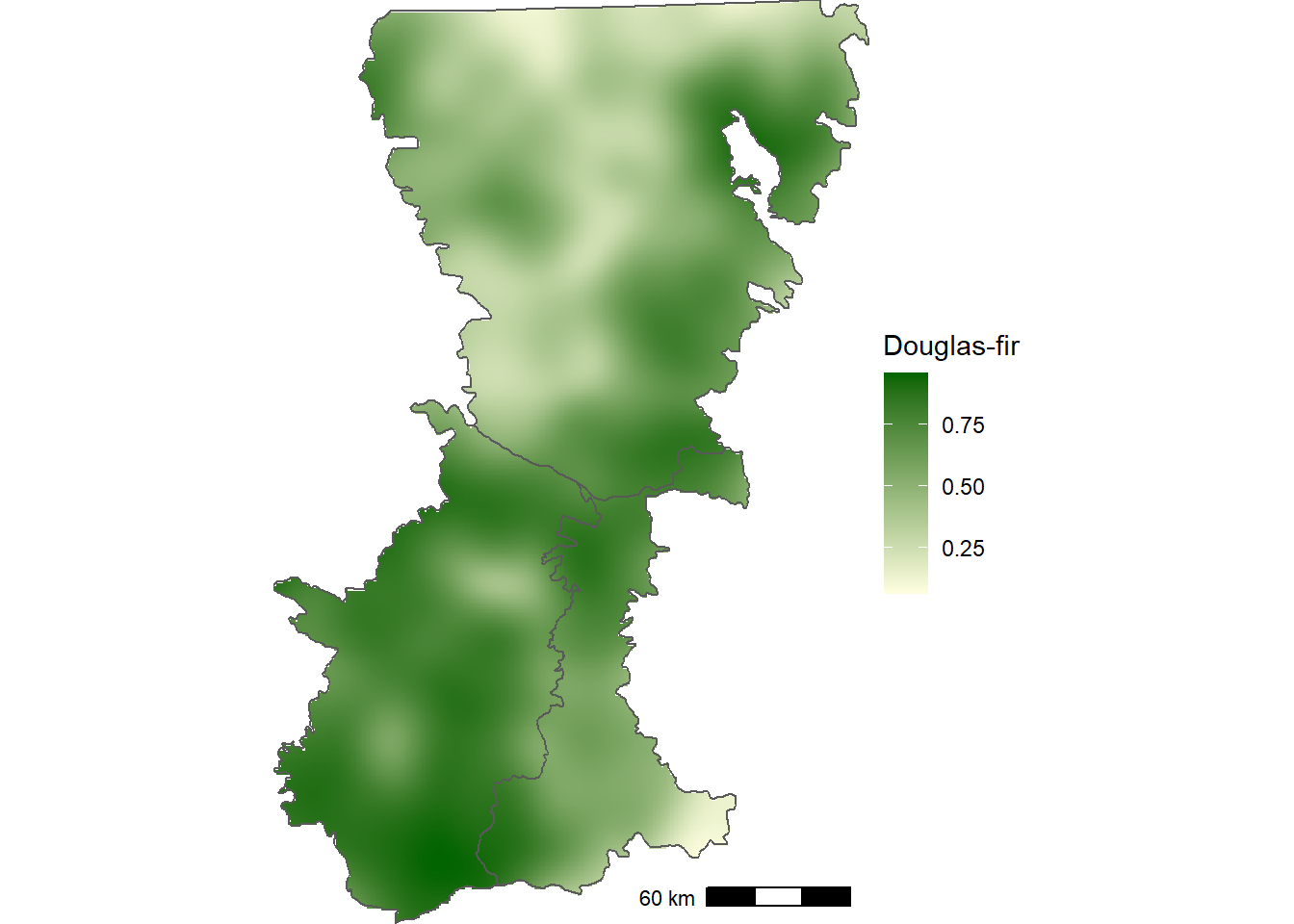
FIGURE 12.4: Smoothed proportion of forest inventory plots with Douglas-fir in the Washington Cascades.
12.2 WorldClim Historical Climate Data
The WorldClim dataset will be used to analyze relationships between tree species and climate. Worldclim is a downscaled global climate dataset available as a 1000 m grid that captures fine-scale variation associated with elevation (Fick and Hijmans 2017). Thus, it is well-suited for rugged terrain like the Washington Cascades. The basic WorClim variables include monthly temperature and precipitation summarized as monthly climatologies over a 30-year period. These monthly data have been used to generate a set of bioclimatic variables that are more suitable as predictors in species distribution models (Table 12.1).
wcbio <- rast("wc2.1_30s_bio_washington.tif")
nlyr(wcbio)
## [1] 19
names(wcbio)
##  [1] "wc2.1_30s_bio_washington_1"
##  [2] "wc2.1_30s_bio_washington_2"
##  [3] "wc2.1_30s_bio_washington_3"
##  [4] "wc2.1_30s_bio_washington_4"
##  [5] "wc2.1_30s_bio_washington_5"
##  [6] "wc2.1_30s_bio_washington_6"
##  [7] "wc2.1_30s_bio_washington_7"
##  [8] "wc2.1_30s_bio_washington_8"
##  [9] "wc2.1_30s_bio_washington_9"
## [10] "wc2.1_30s_bio_washington_10"
## [11] "wc2.1_30s_bio_washington_11"
## [12] "wc2.1_30s_bio_washington_12"
## [13] "wc2.1_30s_bio_washington_13"
## [14] "wc2.1_30s_bio_washington_14"
## [15] "wc2.1_30s_bio_washington_15"
## [16] "wc2.1_30s_bio_washington_16"
## [17] "wc2.1_30s_bio_washington_17"
## [18] "wc2.1_30s_bio_washington_18"
## [19] "wc2.1_30s_bio_washington_19"
The default layer names are replaced by a set of abbreviated codes.
wcbnames <- paste0("bio", c(1, 10:19, 2:9))
names(wcbio) <- wcbnames
wcbnames
##  [1] "bio1"  "bio10" "bio11" "bio12" "bio13" "bio14" "bio15"
##  [8] "bio16" "bio17" "bio18" "bio19" "bio2"  "bio3"  "bio4"
## [15] "bio5" "bio6" "bio7" "bio8" "bio9"| Code | Description |
|---|---|
| bio1 | Annual Mean Temperature |
| bio2 | Mean Diurnal Range |
| bio3 | Isothermality (BIO2/BIO7) (×100) |
| bio4 | Temperature Seasonality |
| bio5 | Max Temperature of Warmest Month |
| bio6 | Min Temperature of Coldest Month |
| bio7 | Temperature Annual Range |
| bio8 | Mean Temperature of Wettest Quarter |
| bio9 | Mean Temperature of Driest Quarter |
| bio10 | Mean Temperature of Warmest Quarter |
| bio11 | Mean Temperature of Coldest Quarter |
| bio12 | Annual Precipitation |
| bio13 | Precipitation of Wettest Month |
| bio14 | Precipitation of Driest Month |
| bio15 | Precipitation Seasonality |
| bio16 | Precipitation of Wettest Quarter |
| bio17 | Precipitation of Driest Quarter |
| bio18 | Precipitation of Warmest Quarter |
| bio19 | Precipitation of Coldest Quarter |
The Washington Cascades ecoregion boundaries are reprojected into a geographic coordinate system with WGS84 datum to match the coordinate reference system of the plot data and the WorldClim data. These polygons are then used to crop and mask the Washington Cascades from the larger Worldclim dataset.
boundary_wgs84 <- st_transform(wacascades, st_crs(wcbio))
wcbio_crop <- crop(wcbio, vect(boundary_wgs84))
wcbio_msk <- mask(wcbio_crop, vect(boundary_wgs84))
The map of maximum temperature during the warmest month of the year highlights the effects of elevation, with the highest temperatures at the fringes of the mountain range and in the larger river valleys. The lowest temperatures occur along the Cascade crest and at the peaks of the large volcanoes (Figure 12.5).
mtwm_df <- rasterdf(wcbio_msk[["bio5"]])
ggplot(data = mtwm_df) +
  geom_raster(aes(x = x,
                  y = y,
                  fill = value)) +
  scale_fill_gradient(name = "Temperature (\u00B0C)",
                      low = "lightyellow",
                      high = "darkred",
                      na.value = NA) +
  geom_sf(data = boundary_wgs84,
          fill = NA) +
  annotation_scale(location = 'br') +
  coord_sf(expand = F) +
  theme_void()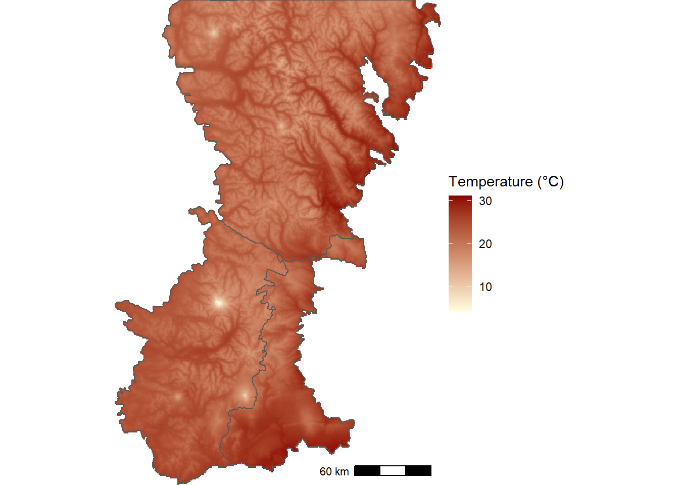
FIGURE 12.5: WorldClim thirty-year climatology of maximum temperature during the warmest month of the year for the Washington Cascades.
The map of precipitation during the wettest month shows the interactions of moist maritime air with topography, with the highest values occurring west of the Cascade Crest and the lowest values in the rain shadow on the eastern slopes (Figure 12.6).
mtwm_df <- rasterdf(wcbio_msk[["bio13"]])
ggplot(data = mtwm_df) +
  geom_raster(aes(x = x,
                  y = y,
                  fill = value)) +
  scale_fill_gradient(name = "Precipitation (mm)",
                      low = "lightblue",
                      high = "darkblue",
                      na.value = NA) +
  geom_sf(data = boundary_wgs84,
          fill = NA) +
  annotation_scale(location = 'br') +
  coord_sf(expand = F) +
  theme_void()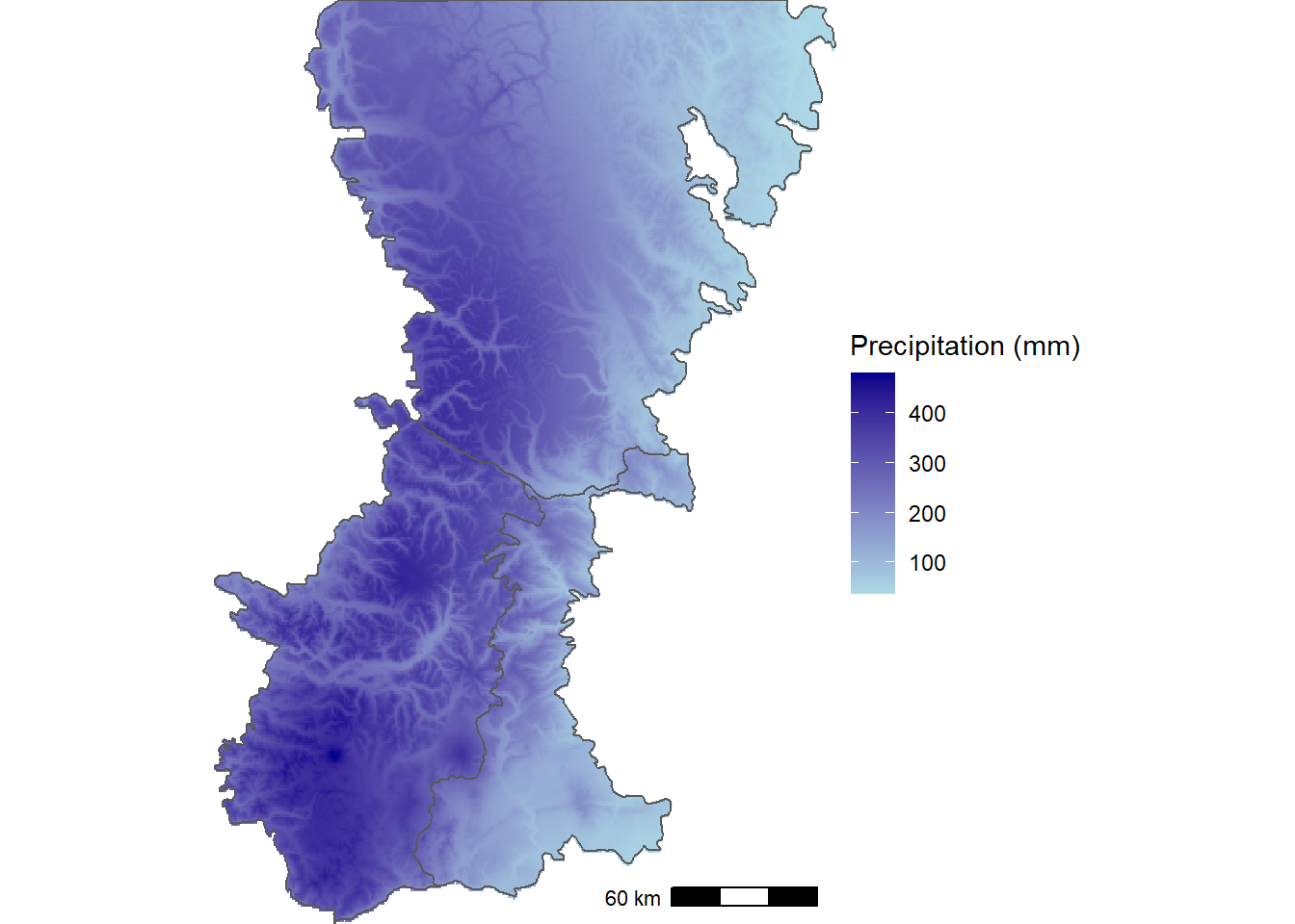
FIGURE 12.6: WorldClim thirty-year climatology of precipitation during the wettest month of the year for the Washington Cascades.
12.3 Modeling the Climate Niche
12.3.1 Subalpine Fir
To prepare the data for modeling, the extract() function is used to obtain climate variables from wcbio_mask for every plot location in the subalpine fir dataset.
abla_bio <- extract(wcbio_msk, vect(abla_pts)) %>%
  bind_cols(abla_pts) %>%
  as.data.frame()
names(abla_bio)
##  [1] "ID"       "bio1"     "bio10"    "bio11"    "bio12"
##  [6] "bio13"    "bio14"    "bio15"    "bio16"    "bio17"
## [11] "bio18"    "bio19"    "bio2"     "bio3"     "bio4"
## [16] "bio5"     "bio6"     "bio7"     "bio8"     "bio9"
## [21] "abla"     "geometry"
To assess the predictive accuracy of the model, a subset of the data needs to be held out from the calibration step and reserved for validation. The data can be split using the sample_frac() function from the dplyr package, where the size argument is the proportion of observations in the sample. There is a similar function called sample_n() that can be used to sample a specific number of observations. The anti_join() function is then used to select the validation points as all the observations in abla_bio that are not present in abla_train.
set.seed(22003)
abla_train <- abla_bio %>%
  sample_frac(size = 0.7)
abla_val <- abla_bio %>%
  anti_join(abla_train, by = "ID")
Boosted regression trees are used to model the relationships between presence/absence of subalpine fir and the 19 bioclimatic variables. BRT is a machine learning method that combines regression trees, which relate species occurrence to a set of climate variables using a series of recursive binary splits, with boosting, an ensemble approach that combines many simple models to improve predictive accuracy (Elith, Leathwick, and Hastie 2008). BRT models can account for non-linear relationships with climate as well as interactions between two or more climate variables. In addition to generating predictions, information about the relative importance of climate predictors can be derived, and climate effects can be visualized using partial regression plots.
BRT models are run using the gbm.step() function from the dismo package. A data frame containing training data is provided along with the indices of the columns to use as the predictor variables (gbm.x) and the response variable (gbm.y). The family = "bernoulli" argument indicates that the model will treat the response as a binomial (presence/absence) variable. The tree.complexity, learning.rate, and bag.fraction arguments control aspects of the gradient boosting algorithm that is used to fit the model. Consult Elith, Leathwick, and Hastie (2008) for more details on these parameters as well as recommended approaches for parameter selection. Here, a set of values that have been determined to yield good predictions with these datasets is used. Other arguments control whether plots and output to the console are automatically produced.
abla_mod <- gbm.step(data = abla_train,
                     gbm.x = 2:20,
                     gbm.y = 21,
                     family = "bernoulli",
                     tree.complexity = 3,
                     learning.rate = 0.01,
                     bag.fraction = 0.5,
                     plot.main = FALSE,
                     verbose = FALSE,
                     silent = TRUE)
After running the model, the summary function can be used to extract information about the relative importance of the predictor variables. The relative importance is based on the number of times a variable is selected for splitting the regression trees weighted by the resulting improvement to the BRT model. The importance values are then rescaled so they sum to 100. For subalpine fir, the mean annual temperature (bio1) has a stronger influence in the model than any other bioclimatic variable followed by mean temperature of the warmest quarter (bio10) mean temperature of the driest quarter (bio9), and precipitation of the warmest quarter (bio18).
abla_imp <- summary(abla_mod, plotit = FALSE)
abla_imp
##         var    rel.inf
## bio1   bio1 36.0562317
## bio10 bio10  8.0557059
## bio9   bio9  6.2651729
## bio18 bio18  6.0591309
## bio3   bio3  5.9187074
## bio17 bio17  5.1232150
## bio15 bio15  4.4587608
## bio14 bio14  4.4537895
## bio8   bio8  4.2289912
## bio11 bio11  3.9730128
## bio4   bio4  3.0952993
## bio5   bio5  2.5050354
## bio6   bio6  1.9115928
## bio12 bio12  1.9019258
## bio2   bio2  1.7437088
## bio7   bio7  1.3484148
## bio16 bio16  1.0302154
## bio13 bio13  0.9892763
## bio19 bio19  0.8818131
Partial residual plots show the nonparametric relationships between subalpine fir occurrence and the predictor variables. They can be generated using the gbm.plot() function from the dismo package. Here, the partial plots for the four most important predictors are shown in a 2 x 2 layout.
Over the range of temperatures in the study area, subalpine fir occurs at the lowest mean annual temperatures (bio1) and declines monotonically with increasing temperature (Figure 12.7). Subalpine fir occurrence also decreases slightly with mean temperature of the warmest quarter (bio10) and precipitation in the warmest quarter (bio18) and is slightly higher at intermediate values of mean temperature during the driest quarter (bio9).
gbm.plot(abla_mod,
         n.plots = 4,
         write.title = FALSE,
         plot.layout = c(2, 2))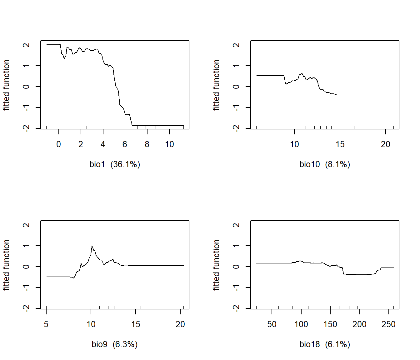
FIGURE 12.7: Partial regression plots showing the response of subalpine fir to WorldClim bioclimatic indices in a boosted regression tree model.
The predicted probability of subalpine fir occurrence can be mapped using the terra prediction function. The SpatRaster object containing the predictor variables is the first argument, followed by the model object. The type = "response" argument is also necessary to transform the predictions to the 0-1 scale, and na.rm = TRUE suppresses predictions outside of the study area where there are no data.
abla_cur <- predict(object = wcbio_msk,
                    model = abla_mod,
                    type = "response",
                    na.rm = TRUE)
Compared to the smoothed map (Figure 12.3), the predicted map based on the WorldClim bioclimatic variables shows much more local variability associated with topography (Figure 12.8). In particular, the species is predicted to be most abundant on high ridges at the Cascade crest and eastward. The circular rings are the upper elevation limits on large volcanoes such as Mount Rainier and Mount Adams.
abla_cur_df <- rasterdf(abla_cur)
ggplot(data = abla_cur_df) +
  geom_raster(aes(x = x,
                  y = y,
                  fill = value)) +
  scale_fill_gradient(name = "Subalpine Fir",
                      low = "lightyellow",
                      high = "darkgreen",
                      na.value = NA) +
  geom_sf(data = boundary_wgs84,
          fill = NA) +
  annotation_scale(location = 'br') +
  coord_sf(expand = F) +
  theme_void()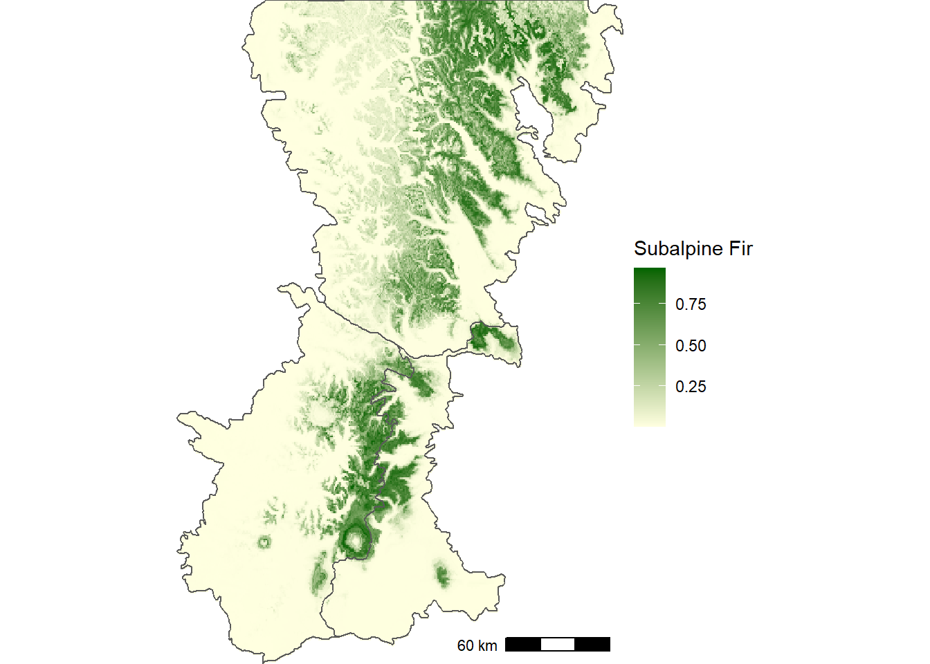
FIGURE 12.8: Predicted probability of subalpine fir occurrence based on historical WorldClim bioclimatic indices.
12.3.2 Douglas-fir
The data preparation and modeling steps are repeated for Douglas-fir.
set.seed(22004)
psme_bio <- extract(wcbio_msk, vect(psme_pts)) %>%
  bind_cols(psme_pts) %>%
  as.data.frame()
psme_train <- psme_bio %>%
  sample_frac(size = 0.7)
psme_val <- psme_bio %>%
  anti_join(abla_train, by = "ID")
psme_mod <- gbm.step(data=psme_train,
                     gbm.x = 2:20,
                     gbm.y = 21,
                     family = "bernoulli",
                     tree.complexity = 3,
                     learning.rate = 0.01,
                     bag.fraction = 0.5,
                     plot.main = FALSE,
                     verbose = FALSE,
                     silent = TRUE)
The variable importance ranking is different for Douglas-fir compared to Subalpine Fir. The two most important variables, maximum temperature of the warmest month (bio5) and mean temperature of the warmest quarter (bio10) have considerably higher relative importance than the rest of the variables.
psme_imp <- summary(psme_mod, plotit = FALSE)
psme_imp
##         var    rel.inf
## bio5   bio5 19.3455300
## bio10 bio10 13.5939889
## bio14 bio14  7.3627926
## bio17 bio17  7.0770029
## bio18 bio18  6.0665693
## bio4   bio4  5.4373063
## bio15 bio15  5.2734444
## bio3   bio3  4.9268249
## bio9   bio9  4.1113149
## bio1   bio1  3.9882327
## bio2   bio2  3.7682976
## bio6   bio6  3.4319576
## bio12 bio12  3.0354558
## bio11 bio11  2.9986297
## bio8   bio8  2.8962037
## bio7   bio7  2.8731305
## bio16 bio16  1.4739840
## bio19 bio19  1.3695103
## bio13 bio13  0.9698239
The relationships between Douglas-fir and these two variables are unimodal, with species occurrence peaking across a range of optimal temperatures and decreasing at cooler and warmer temperatures (Figure 12.9). Douglas-fir also has unimodal relationships with precipitation in the driest month (bio14) and precipitation in the driest quarter (bio17).
gbm.plot(psme_mod,
         n.plots = 4,
         write.title = FALSE,
         plot.layout = c(2, 2))
FIGURE 12.9: Partial regression plots showing the response of Douglas-fir to WorldClim bioclimatic indices in a boosted regression tree model.
The predicted occurrence map shows that Douglas-fir is widespread throughout the southern part of the Washington Cascades but is confined to lower-elevation valleys in the northern part of the region (Figure 12.10).
psme_cur <- predict(object = wcbio_msk,
                    model = psme_mod,
                    type = "response",
                    na.rm = TRUE)
psme_cur_df <- rasterdf(psme_cur)
ggplot(data = psme_cur_df) +
  geom_raster(aes(x = x,
                  y = y,
                  fill = value)) +
  scale_fill_gradient(name = "Douglas-fir",
                      low = "lightyellow",
                      high = "darkgreen",
                      na.value = NA) +
  geom_sf(data = boundary_wgs84,
          fill = NA) +
  annotation_scale(location = 'br') +
  coord_sf(expand = F) +
  theme_void()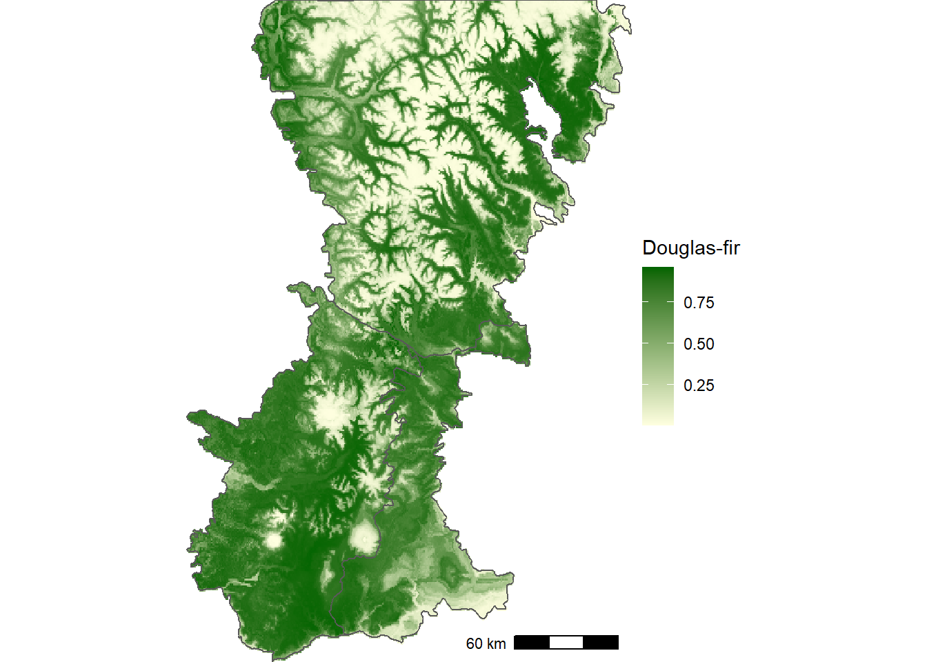
FIGURE 12.10: Predicted probability of Douglas-fir occurrence based on historical WorldClim bioclimatic indices.
12.4 Accuracy Assessment
To understand how accurate the species distribution model predictions are, the predict() function is used to generate predictions based on the validation dataset. In this example, the predict() method for gbm objects is invoked, requiring different arguments than the previous examples, which used the predict() method for SpatRaster objects. The first argument is the gbm model, and the newdata argument is used to specify the abla_val data frame, which was created earlier when the full dataset was split into training and validation sets. The vector of predicted values is combined with the observed values from the abla_val data frame, and the prediction() function from the ROCR package is used to generate a prediction object that can be used for computing accuracy statistics.
abla_pred <- predict(abla_mod,
                     newdata = abla_val,
                     type = "response")
abla_predobs <- prediction(abla_pred, abla_val$abla)
Although the observations are binary, the output of the model is a continuous probability between zero and one. The receiver operating characteristic curve (ROC) is commonly used to evaluate the predictive capability of such a model. The ROC is generated by using the predicted probability to classify presence or absence over a range of cutoff values and exploring the tradeoff between predictions of presence and absence. At the extreme, if all predicted probabilities less than one are assumed to be positive, then all points are classified as present. In this case, the model will correctly predict all the locations where subalpine fir is actually present but fail to predict any of the points where it is actually absent. The reverse is true if zero is used as the threshold and all points are classified as absent.
The ROC curve describes the changes in true positive rates and false positive rates over all possible cutoff values. The performance() function in the ROCR package is used to generate a performance object that includes these two measures.
abla_roc = performance(abla_predobs,
                       measure = "tpr",
                       x.measure = "fpr")
class(abla_roc)
## [1] "performance"
## attr(,"package")
## [1] "ROCR"
The performance object could be visualized using a generic plot() method, but this example will show how to extract the underlying data and generate an ROC curve with ggplot(). The ROCR package uses the S4 object system. Details of S4 are outside the scope of this book, but at the most basic level, these objects require new functions to visualize and extract their components, which are stored in “slots”.
slotNames(abla_roc)
## [1] "x.name"       "y.name"       "alpha.name"
## [4] "x.values"     "y.values"     "alpha.values"
The slot() function can be used to access the slots in an S4 object. The x.values and y.values contain the false positive rates and the true positive rates for the ROC curve. These data are stored as lists with a single element. Double brackets are used to subscript these list elements and return numeric vectors, which are combined into a data frame.
abla_fpr <- slot(abla_roc, "x.values")[[1]]
abla_tpr <- slot(abla_roc, "y.values")[[1]]
abla_aucplot <- data.frame(abla_fpr, abla_tpr)
This data frame can be used with ggplot() to graph the ROC curve. As the false positive rate (equal to one minus the true negative rate) decreases, the true positive rate also decreases (Figure 12.11).
ggplot(data = abla_aucplot) +
  geom_line(aes(x = abla_fpr,
                y = abla_tpr),
            col = "red") +
  labs(x = "False Positive Rate",
       y = "True Positive Rate") +
  geom_abline(slope = 1, intercept = 0) +
  scale_x_continuous(expand = c(0.005, 0)) +
  scale_y_continuous(expand = c(0.005, 0)) +
  coord_fixed() +
  theme_bw()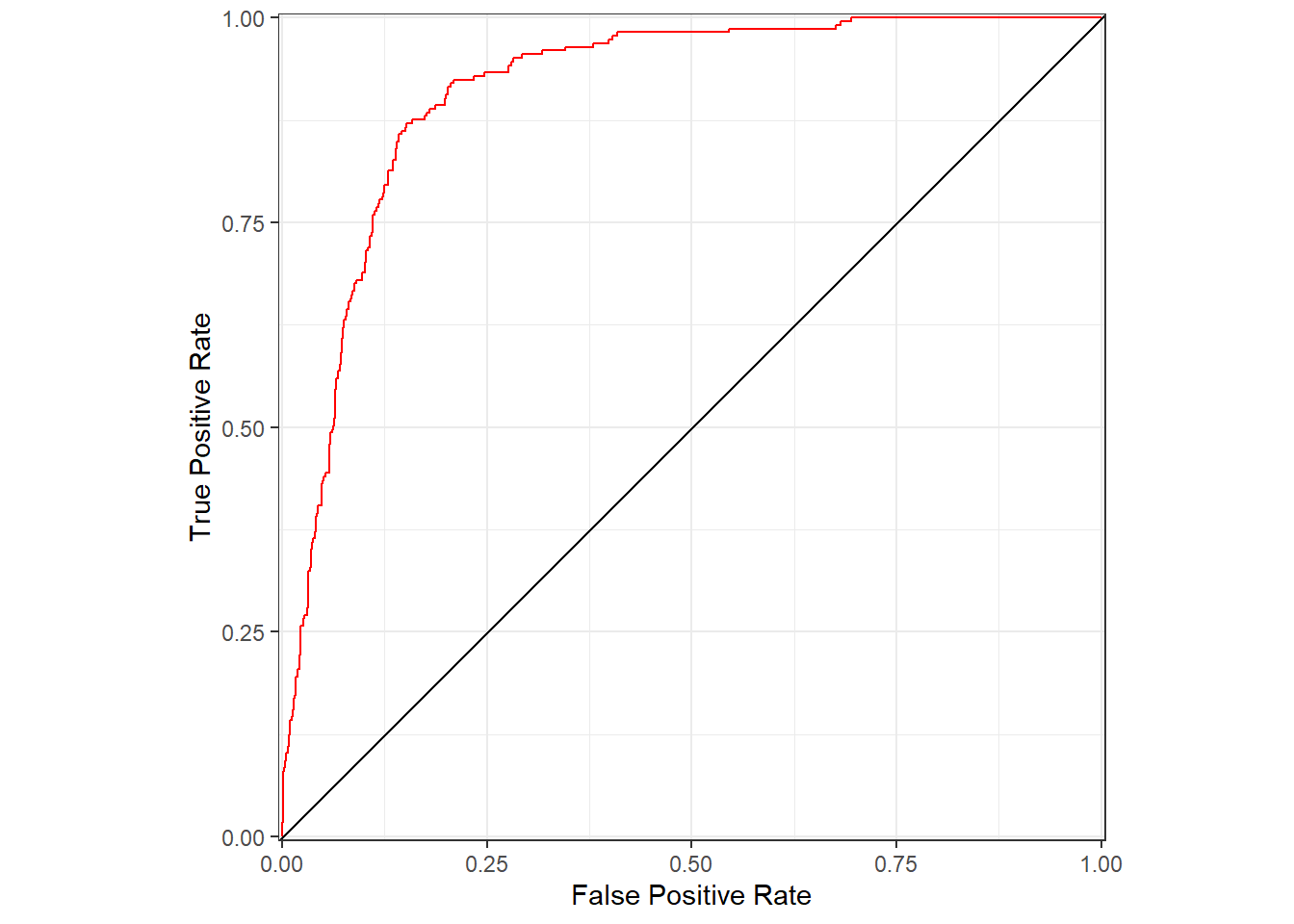
FIGURE 12.11: Area under the receiver operating characteristics (ROC) curve for predictions of subalpine fir occurrence based on WorldClim bioclimastic indices.
Another way to visualize these relationships is to graph the overall accuracy, true positive rate, and true negative rate as a function of the cutoff used for prediction. The performance() function is used to create performance objects containing these three statistics. The values are then extracted and combined into a long-format data frame.
abla_all = performance(abla_predobs,
                       measure = "acc")
abla_pos = performance(abla_predobs,
                       measure = "tpr")
abla_neg = performance(abla_predobs,
                       measure = "tnr")
cutoff <- slot(abla_all, "x.values")[[1]]
totacc <- slot(abla_all, "y.values")[[1]]
posacc <- slot(abla_pos, "y.values")[[1]]
negacc <- slot(abla_neg, "y.values")[[1]]
abla_accplot <- data.frame(cutoff,
                           totacc,
                           posacc,
                           negacc) %>%
  pivot_longer(cols = one_of("totacc",
                             "posacc",
                             "negacc"),
               values_to = "accval",
               names_to = "accstat")
The results suggest that a cutoff value around 0.25 would be effective for classifying presence or absence based on the predictions (Figure 12.12) . The overall accuracy is close to the maximum, and the true negative and true positive rates are balanced and relatively high.
ggplot(data = abla_accplot) +
  geom_line(aes(x = cutoff,
                y = accval,
                col = accstat)) +
    labs(x = "Classification Cutoff",
         y = "Classification Accuracy",
         color = "Accuracy Statistic") +
  scale_color_discrete(labels = c("True Negative Rate",
                                 "True Positive Rate",
                                 "Overall Accuracy")) +
  scale_x_continuous(expand = c(0.005, 0)) +
  scale_y_continuous(expand = c(0.005, 0)) +
  coord_fixed() +
  theme_bw()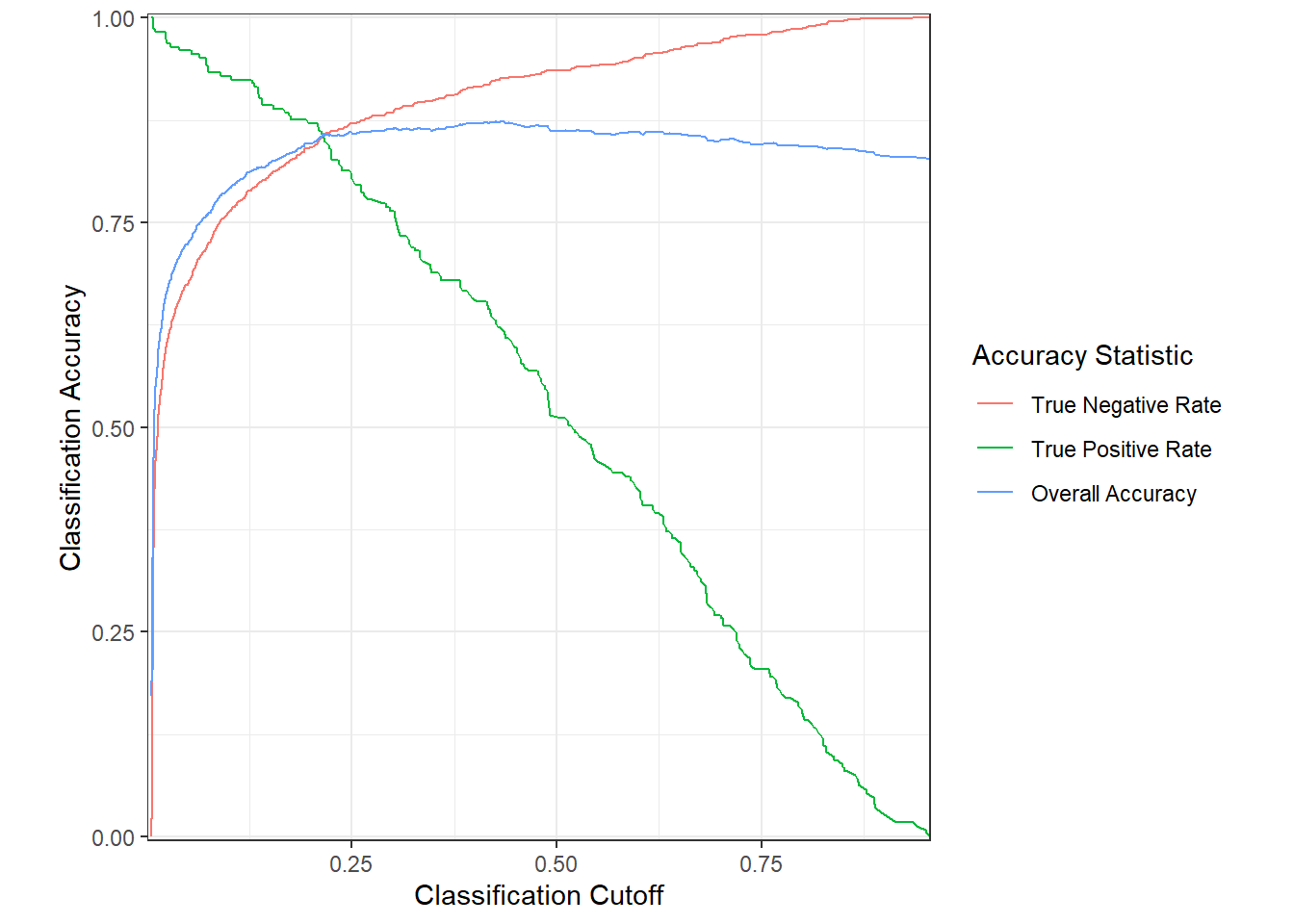
FIGURE 12.12: Overall accuracy, true positive rate, and true negative rate for predictions of subalpine fir occurrence based on WorldClim bioclimastic indices.
The area under the ROC curve, often abbreviated as the AUROC or just the AUC, is frequently used as an index of the predictive power of a probabilistic model for binary data like species presence/absence. Values range from a minimum of 0.5 to a maximum of 1.0. The AUC statistic can be calculated using the performance() function.
abla_aucval <- performance(abla_predobs, measure = "auc")
slot(abla_aucval, "y.values")[[1]]
## [1] 0.910495
The AUC for the subalpine fir model is 0.91, which is relatively high value and indicates that predictions are accurate over a range of cutoff values.
12.5 Climate Change Projections
The WorldClim dataset also includes projected future climate grids based on the outputs of general circulation models (GCMs) from the Coupled Model Intercomparison Project (CMIP) version 6. This example uses a projection for 2061-2080 from the Max Planck Institute Earth System Model (MPI-ESM1.2). It is based on RCP4.5 global forcing pathway, which assumes that carbon dioxide (CO2) emissions will start to decline before 2045 and reach approximately half of their 2050 levels by 2100. The variables are the same bioclimatic indices that were computed for the historical climatology. The data are read into a raster object, assigned layer names, and cropped and masked to the Washington Cascades study area.
wcproj <- rast("wc2.1_30s_bioc_MPI-ESM1-2-HR_ssp245_2061-2080_wa.tif")
nlyr(wcproj)
## [1] 19
wcbnames <- paste0("bio", 1:19)
names(wcproj) <- wcbnames
wcproj_crop <- crop(wcproj, vect(boundary_wgs84))
wcproj_msk <- mask(wcproj_crop, vect(boundary_wgs84))
The terra predict() function is used to generate predictions of subalpine fir distribution under the future climate scenario. The object argument is used to specify the raster with projected climate variables. This raster must have the same layer names as the original variables that were used to train the model. The output, abla_proj, is combined with the predictions under current conditions, abla_cur, to create a multi-layer raster.
abla_proj <- predict(object = wcproj_msk,
                     model = abla_mod,
                     type = "response",
                     na.rm = TRUE)
abla_chg <- c(abla_cur, abla_proj)
names(abla_chg) <- c("Current", "Future")
To display the predictions as binary presence or absence outcomes, the probabilities are classified using a cutoff value of 0.25.
abla_clas <- ifel(abla_chg > 0.25, 1, 0)Comparing these two maps shows that the projected range of subalpine fir is considerably smaller under a future, warmer climate, with the species restricted to the highest elevations in the Washington Cascades (Figure 12.13).
abla_clas_df <- rasterdf(abla_clas)
ggplot(data = abla_clas_df) +
  geom_raster(aes(x = x,
                  y = y,
                  fill = as.character(value))) +
  scale_fill_manual(name = "Subalpine Fir",
                      values = c("lightyellow",
                                 "darkgreen"),
                      labels = c("absent",
                                 "present"),
                      na.translate = FALSE) +
  facet_wrap(~ variable) +
  geom_sf(data = boundary_wgs84,
          fill = NA) +
  coord_sf(expand = F) +
  theme_void()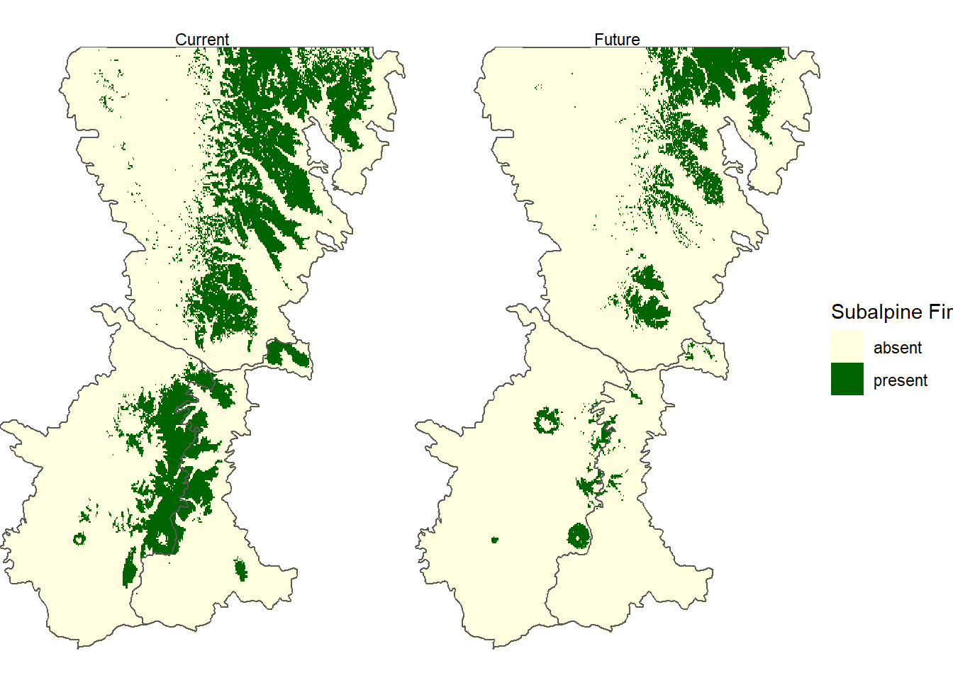
FIGURE 12.13: Predicted probability of subalpine fir occurrence based on future (2061-2080) WorldClim bioclimatic indices.
In addition to generating maps, the data frame generated by the rasterdf() function can also be used to create other types of graphs based on the values in a raster dataset. In this example, histograms of current and future mean annual temperatures show that the distribution of temperatures will be considerably higher under the future climate scenario (Figure 12.14).
annmean <- c(wcbio_msk[["bio1"]], wcproj_msk[["bio1"]])
names(annmean) <- c("Current", "Future")
annmean_df <- rasterdf(annmean)

ggplot(data = annmean_df) +
  geom_histogram(aes(x = value), bins = 20) +
  labs(x = "Mean Annual Temperature (\u00B0C)",
       y = "Count of observations") +
  facet_wrap(~ variable, ncol = 1) +
  theme_bw()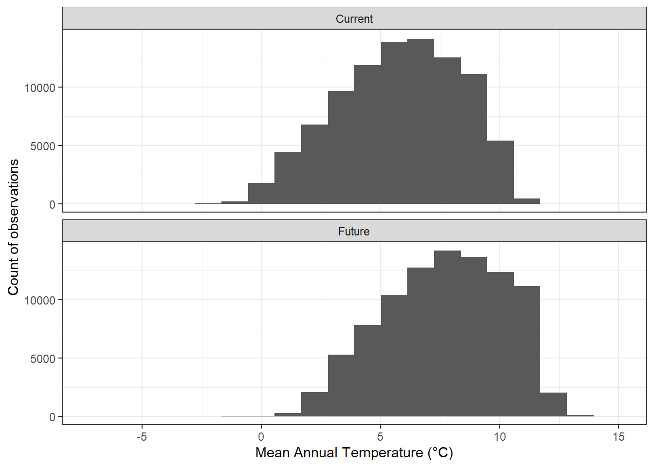
FIGURE 12.14: Histogram of current and projected future mean annual temperatures for the Washington Cascades.
12.6 Practice
Carry out an accuracy assessment of the species distribution model for Douglas-fir and compare the results to those obtained for subalpine fir.
Predict the future distribution of Douglas-fir using the climate projections and compare the results with the projected future distribution of subalpine fir.
Generate a map that shows where the distribution of subalpine fir is projected to expand, contract, and remain the same under future climate projections. Then generate a similar map for Douglas-fir and compare the two.