Chapter 9 Combining Vector Data with Continuous Raster Data
To conduct geospatial analyses, it is usually necessary to combine data from multiple sources. Often, this involves using vector data as well as raster data. For example, geospatial climate and weather data are typically provided as rasters, while geospatial data on the demographics of human populations are typically referenced to polygons. To understand how different populations subgroups may be exposed to different climate and meteorological hazards, it is necessary to integrate data with fundamentally different geospatial structures.
The next two chapters will provide several examples of how vector and raster data can be combined in R to carry out common types of analyses. This chapter will present several analyses using the PRISM dataset (http://www.prism.oregonstate.edu). This is a widely-used interpolated climate dataset for the United States that is based on data from meteorological stations combined with other ancillary datasets such as elevation (Daly et al. 2002).
library(tidyverse)
library(sf)
library(terra)
library(prism)
library(tigris)
9.1 Accessing Data with R Packages
In previous chapters, various functions have been used to import data into R and convert them into appropriate objects for tabular data and geospatial data in vector and raster formats. This chapter will use a different approach for bringing data into R. County boundaries and gridded climate and meteorological data will be imported directly from online archives using two R packages specifically designed to facilitate data access: tigris (Walker 2022) and prism (Edmund and Bell 2020).
To start, we will use the tigris package to download a county shapefile similar to the one that was used in Chapter 8 on coordinate reference systems. The county() function is used with the cb = TRUE argument to indicate that a dataset with generalized county boundaries will be downloaded and resolution = '20m' to indicate the scale (1:20 million) of the data. The function returns an sf object that contains columns with state and county names, codes, and areas along with geometry information for each county.
county <- counties(cb = TRUE,
                   resolution = '20m')
class(county)
glimpse(county)
The STATEFP and GEOID fields are initially read in as characters, but they are convered to numbers to make it easier to join with the zonal summary table later on. Then, as in Chapter 8, the dataset is filtered down to only the 48 conterminous United States.
county <- county %>%
  mutate(state = as.numeric(STATEFP),
         fips = as.numeric(GEOID)) %>%
  filter(state != 2, state != 15, state < 60)
As discussed in Chapter 8, it is important to know the coordinate reference system of the data. These county data are in a geographic coordinate system (longitude and latitude) with a NAD83 datum.
writeLines(st_crs(county)$WktPretty)
## GEOGCS["NAD83",
##     DATUM["North_American_Datum_1983",
##         SPHEROID["GRS 1980",6378137,298.257222101]],
##     PRIMEM["Greenwich",0],
##     UNIT["degree",0.0174532925199433,
##         AUTHORITY["EPSG","9122"]],
##     AXIS["Latitude",NORTH],
##     AXIS["Longitude",EAST],
##     AUTHORITY["EPSG","4269"]]
The prism package automates data downloading and importing of PRISM climate data. Setting options(prism.path = ".") downloads and stores the data in the current working directly. To download the data to a different location in the file system, a directory path can be specified here instead. The code in this example downloads the 30-year climatology of annual precipitation for the conterminous U.S. using the get_prism_normals() function. The type = 'ppt' argument specifies that precipitation data will be downloaded. Other types of data that can be downloaded are shown on the help pages for get_prism_normals() and other prism functions. The resolution argument can be used to select either 4km or 800m grids. The annual = TRUE argument selects annual instead of monthly summaries, and the keepZip = TRUE argument saves the downloaded ZIP archives.
options(prism.path = ".")
get_prism_normals(type = 'ppt',
                  resolution = '4km',
                  annual = T,
                  keepZip = TRUE)
The get_prism_monthlys() function can similarly be used to download monthly meteorological summaries for a specific range of years and months.
get_prism_monthlys(type = 'ppt',
                   years = 2018,
                   mon=1:12,
                   keepZip = TRUE)
The prism package also has functions for managing these downloaded data. The prism_archive_ls() function produces a vector containing the names of all downloaded PRISM datasets.
prism_files <- prism_archive_ls()
prism_files
##  [1] "PRISM_ppt_30yr_normal_4kmM3_annual_bil"
##  [2] "PRISM_ppt_stable_4kmM3_201801_bil"
##  [3] "PRISM_ppt_stable_4kmM3_201802_bil"
##  [4] "PRISM_ppt_stable_4kmM3_201803_bil"
##  [5] "PRISM_ppt_stable_4kmM3_201804_bil"
##  [6] "PRISM_ppt_stable_4kmM3_201805_bil"
##  [7] "PRISM_ppt_stable_4kmM3_201806_bil"
##  [8] "PRISM_ppt_stable_4kmM3_201807_bil"
##  [9] "PRISM_ppt_stable_4kmM3_201808_bil"
## [10] "PRISM_ppt_stable_4kmM3_201809_bil"
## [11] "PRISM_ppt_stable_4kmM3_201810_bil"
## [12] "PRISM_ppt_stable_4kmM3_201811_bil"
## [13] "PRISM_ppt_stable_4kmM3_201812_bil"
Each PRISM dataset consists of multiple files and is stored in a separate folder, which conveniently has the exact same name as the dataset. The files include a bit interleaved by line (BIL) image as well as other auxiliary files containing projection and header information along with metadata. The following code generates a vector of paths to the BIL files. The “.” at the beginning of the path indicates that the folder location is relative to the user’s working directory. The rast() function is used to create a SpatRaster object containing the 30-year precipitation normals (the first element in the prism_paths vector), and another containing monthly precipitation rasters for 2018 (elements two through thirteen in the prism_paths vector).
prism_paths <- file.path(".",
                         prism_files,
                         paste0(prism_files, ".bil"))
prism_p30 <- rast(prism_paths[1])
prism_prec_2018 <- rast(prism_paths[2:13])
Packages like tigris and prism are designed to provide easy access to standard datasets. Instead of downloading the data externally and then importing it into R, these packages download the data within the R session. The tigris package directly imports U.S. Census datasets into R objects, whereas the prism package manages a library of downloaded raster datasets. There are numerous other packages available that provide access to a variety of datasets.
Accessing remote data through packages can be very convenient. It also helps to make scientific workflows more distributable and reproducible because data acquisition and analysis can be integrated in a single R script. However, ingtegrating remote data access into analytical workflows may not always be the best approach. Downloading the data each time a script is run can be time-consuming, and it may not be possible to run the script if there are changes to the external data server, the server is inaccessible, or the internet bandwidth is limited. In some cases, it may be more feasible to download the data outside of the R session and then store and access them locally.
9.2 Zonal Statistics
Zonal statistics are a type of polygon-on-raster overlay in which the values in the raster dataset are summarized within each polygon. The terra package has a zonal() function for this type of calculation, but it requires a bit more data preparation than when running zonal statistics in other GIS software such as ArcGIS. This example will address the problem of summarizing mean annual precipitation for every county in the United States.
To calculate zonal statistics, it is necessary to convert the vector polygon dataset of counties to a raster dataset in which each raster cell is coded with the 5-digit FIPS code of the corresponding county. The rasterize() function is used to convert vector to raster data. The first argument is the county dataset to summarize wrapped in the vect() function to convert it to the terra vector data format. The second argument is a raster dataset to provide parameters for the conversion. The output will match the CRS, extent, origin, numbers of rows and columns, and cell size of the prism_p30 dataset. This matching is essential so that the rasterized counties and the PRISM precipitation grid can be combined in the next step. The field = "fips" argument indicates which column in the county vector dataset will be used to assign values to the raster cells in the output.
cnty_ras <- rasterize(vect(county),
                      prism_p30,
                      field = "fips")
summary(cnty_ras)
##       fips
##  Min.   : 1001
##  1st Qu.:18177
##  Median :31091
##  Mean   :30738
##  3rd Qu.:46019
##  Max.   :56045
##  NA's   :45857
Zonal statistics are generated wtih the zonal() function. The first argument specifies the raster layer to summarize and the second argument specifies the zones to use for summarization. The fun = "mean" argument indicates the summary function to use for each zone, and the na.rm = TRUE argument is passed to the mean() function to remove NA values prior to summarization. The output is a data frame with one row for each county. The precipitation summary column initially has the long file name of the original image dataset, but is renamed as precip for simplicity.
cnty_p30 <- zonal(prism_p30,
                  cnty_ras,
                  fun = "mean",
                  na.rm = TRUE)
summary(cnty_p30)
##       fips       PRISM_ppt_30yr_normal_4kmM3_annual_bil
##  Min.   : 1001   Min.   :  78.88
##  1st Qu.:19041   1st Qu.: 763.73
##  Median :29205   Median :1095.83
##  Mean   :30625   Mean   :1026.01
##  3rd Qu.:45087   3rd Qu.:1277.06
##  Max.   :56045   Max.   :3068.14
cnty_p30 <- rename(cnty_p30,
                   precip = 2)
When processing data, it is always advisable to run basic checks to ensure that the results make sense. In this case, it is expected that the number of counties (rows) in the cnty_p30 datasets containing zonal summaries should match the number of counties in the original county dataset. However, this is not the case. There are fewer counties in the summary data table than there are counties in the polygon file.
dim(cnty_p30)
## [1] 3101    2
dim(county)
## [1] 3108   15
setdiff(county$fips,
        cnty_p30$fips)
## [1] 51580 51600 51678 51685 51683 51570 51610
9.3 Zone Size and Raster Cell Size
One of the most effective ways to assess data processing errors is through visualization. In this case, mapping the zonal summaries may reveal where data are missing. However, when the zonal summaries are joined to the county polygons and mapped, there are no obviously visible counties with missing data (Figure 9.1).
cnty_join1 <- left_join(county,
                        cnty_p30,
                        by = "fips")

ggplot(data = cnty_join1) +
  geom_sf(aes(fill = precip), size = 0.1) +
  scale_fill_continuous(name = "Precip (mm)") +
  theme_bw() +
  theme(legend.position = "bottom")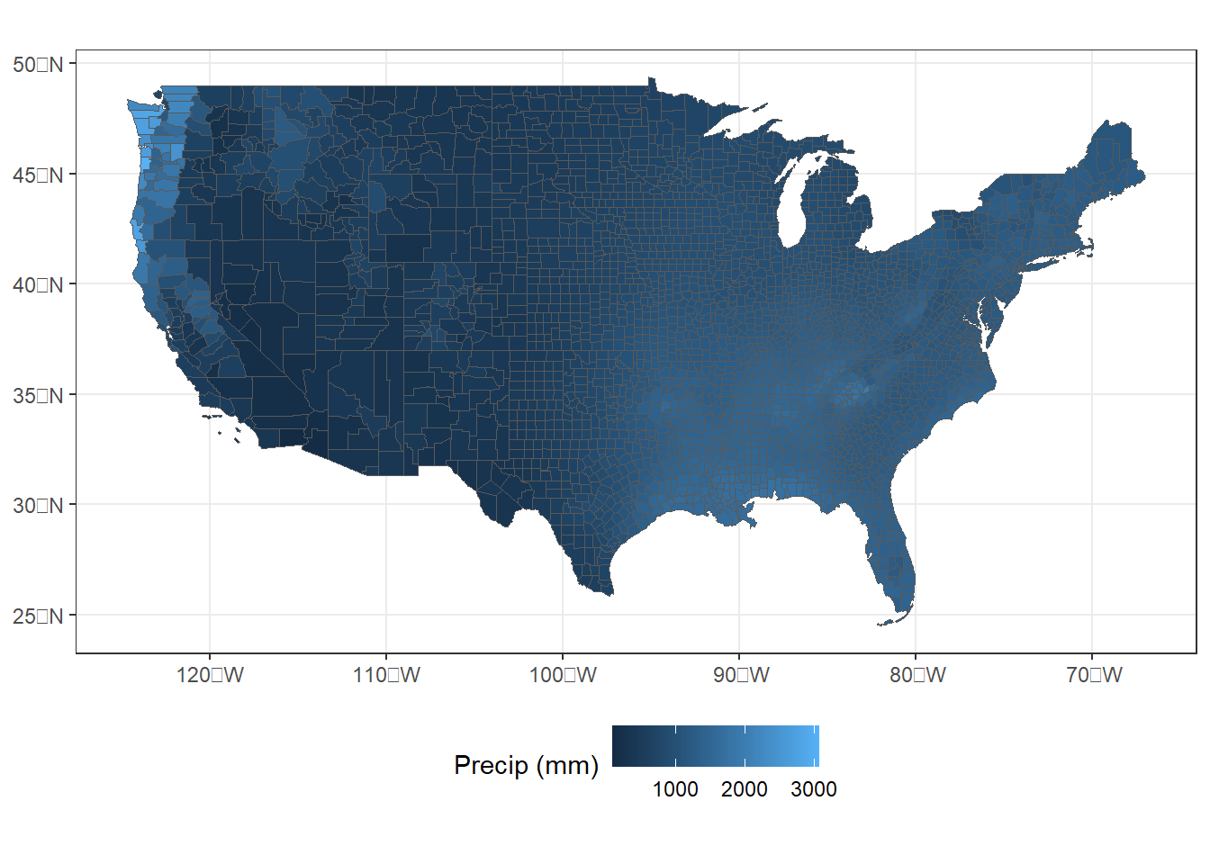
FIGURE 9.1: County-level zonal summaries of precipitation data from the PRISM dataset.
To make the map more readable, the scale_fill_distiller() function can be used to specify a yellow-to-green-to-blue color palette, change the direction so that areas with more precipitation are blue, and use a logarithmic scale instead of a linear scale for precipitation (Figure 9.2).
ggplot(data = cnty_join1) +
  geom_sf(aes(fill = precip), size = 0.1) +
  scale_fill_distiller(name = "Precip (mm)",
                       palette = "YlGnBu",
                       direction = 1,
                       trans = "log",
                       breaks = c(100, 300, 1000, 3000)) +
  theme_bw() +
  theme(legend.position = "bottom")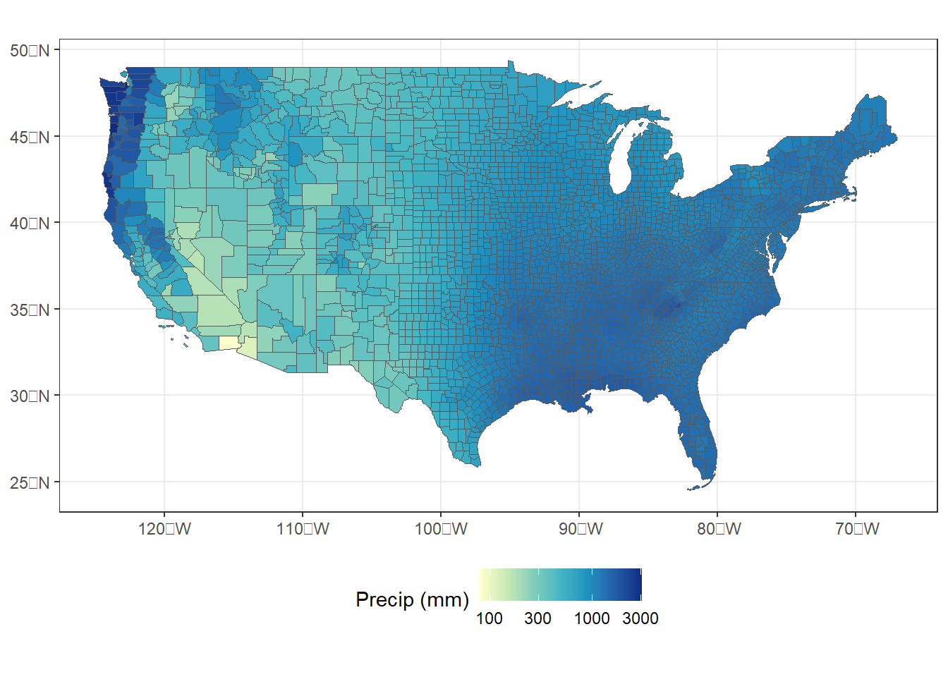
FIGURE 9.2: County-level zonal summaries of precipitation data from the PRISM dataset with a logarithmic transformation.
Displaying precipitation on a logarithmic scale is appropriate in this case because the data are heavily skewed, with most counties having relatively low values and a few having extremely large values. The logarithmic transformation stretches the lower values over a broader range of colors, which make the variation easier to see. However, the logarithm of zero is undefined and will return an NA value in R, so this approach does not work when there are zero values in the data.
Another way to look for the missing counties is to use the setdiff() function to return a vector of county FIPS codes that are present in the county dataset, but not the cnty_p30 dataset. Note that all the missing counties have a state FIPS code of 51, which is Virginia.
setdiff(county$fips, cnty_p30$fips)
## [1] 51580 51600 51678 51685 51683 51570 51610
The next step is to zoom in and take a closer look at just Virginia. The filter() function selects only the counties in Virginia, and a new map is generated (Figure 9.3).
va_join1 <- filter(cnty_join1,
                   STATEFP == "51")

ggplot(data = va_join1) +
  geom_sf(aes(fill = precip), size = 0.1) +
  scale_fill_distiller(name = "Precip (mm)",
                       palette = "YlGnBu",
                       direction = 1,
                       trans = "log",
                       breaks = c(1000, 1150, 1300)) +
  theme_bw() +
  theme(legend.position = "bottom")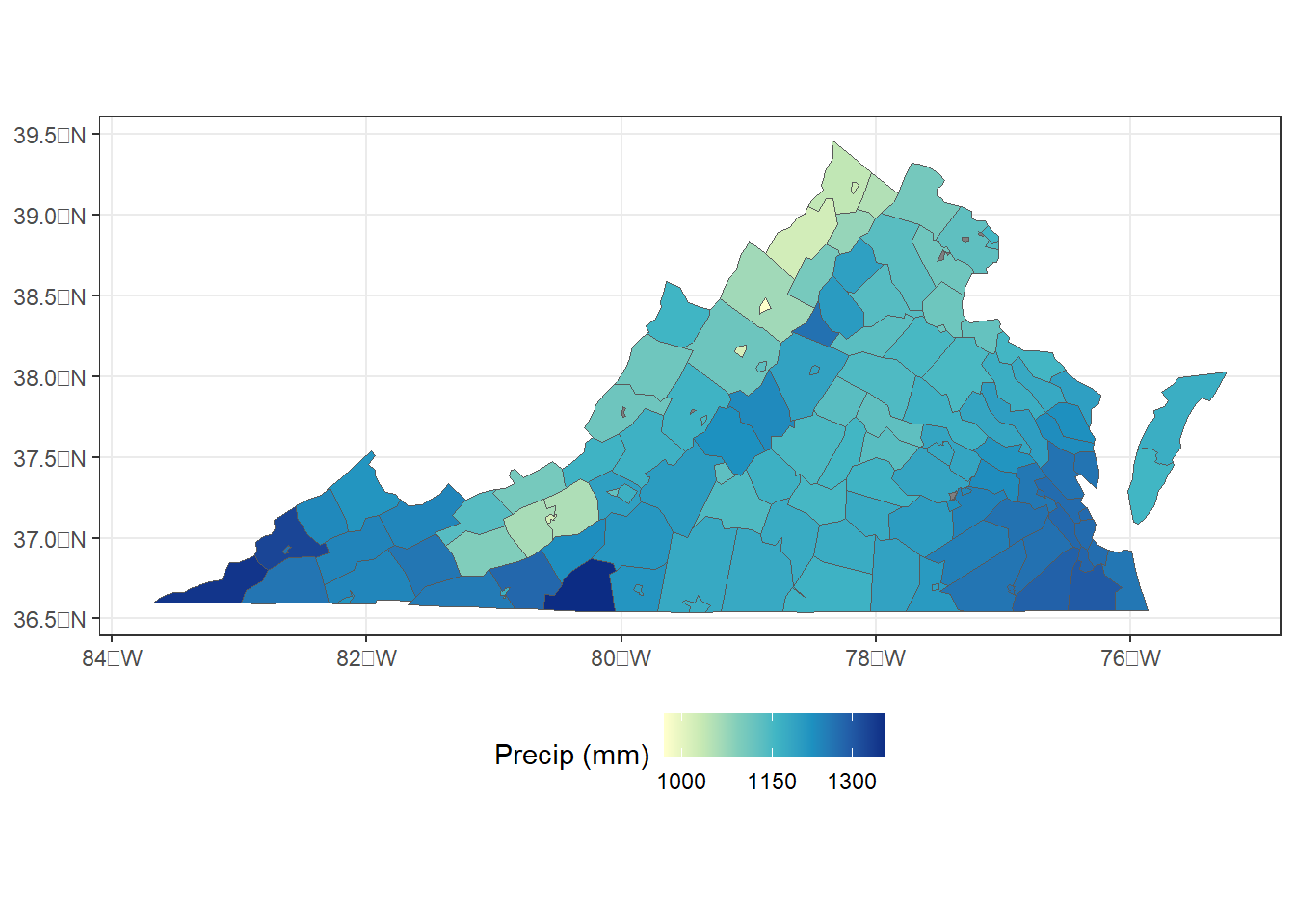
FIGURE 9.3: County-level zonal summaries of precipitation data from the PRISM dataset for Virginia.
Virginia is unique among states in that it has many small, independent cities that are governed separately from the surrounding counties and are therefore assigned their own county FIPS codes. However, it’s still not clear where the missing data are located. To zoom in further to a portion of Northern Virginia, the xlim and ylim arguments can be specified in the coord_sf() function (Figure 9.4).
ggplot(data = va_join1) +
  geom_sf(aes(fill = precip), size = 0.25) +
  coord_sf(xlim = c(-77.6, -77.0),
           ylim = c(38.6, 39.1)) +
  scale_fill_distiller(name = "Precip (mm)",
                       palette = "YlGnBu",
                       direction = 1,
                       trans = "log",
                       breaks = c(1000, 1150, 1300)) +
  theme_bw()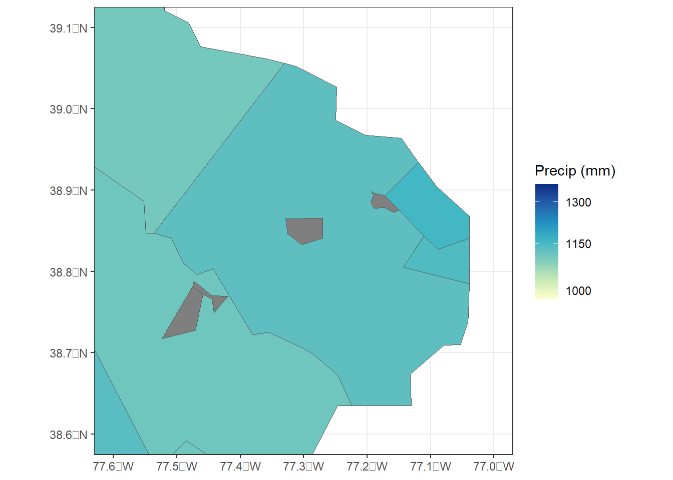
FIGURE 9.4: County-level zonal summaries of precipitation data from the PRISM dataset for northern Virginia.
Now we can see several small cities with missing precipitation data. Why did this happen? When the counties were rasterized to a 4 km grid to match the precipitation data, the center point of each 4 km grid cell was sampled and assigned it the FIPS code of the county that it fell within. However, if a county is very small or narrow, it is possible that no grid center point will fall within its boundaries. In this situation, the county ends up excluded from the zonal summary.
The simplest way to deal with this problem is to use a finer sampling grid to generate the zonal statistics. This can be accomplished with the following steps. The disagg() function is used to reduce the cell size of the PRISM data by a factor of four, changing the cell size to approximately 1 km. Bilinear resampling is used to conduct linear interpolation between the center points of the 4 km grid cells to estimate values at the 1 km resolution. Then, the new 1 km grid is used to rasterize the county dataset, and the zonal() function is run using the 1 km county and precipitation rasters.
prism_p30_1km <- disagg(prism_p30,
                        fact = 4,
                        method = "bilinear")
cnty_ras_1km <- rasterize(vect(county),
                          prism_p30_1km,
                          field = "fips")
cnty_p30_1km <- zonal(prism_p30_1km,
                      cnty_ras_1km,
                      fun = "mean",
                      na.rm=T)
summary(cnty_p30_1km)
##       fips       PRISM_ppt_30yr_normal_4kmM3_annual_bil
##  Min.   : 1001   Min.   :  78.39
##  1st Qu.:19045   1st Qu.: 765.71
##  Median :29212   Median :1096.10
##  Mean   :30672   Mean   :1026.02
##  3rd Qu.:46008   3rd Qu.:1276.20
##  Max.   :56045   Max.   :3041.39
cnty_p30_1km <- rename(cnty_p30_1km,
                       precip = 2)
There is also a resample() function that does essentially the same thing, but allows the user to specify a different grid for the resampling rather than calculating resolution as a factor of the current grid cell size. The resample() function is used in situations where one raster needs to be adjusted to match another raster with a different grid cell size or grid origin.
Now the zonal summary table contains the same number of records as the county file.
dim(cnty_p30_1km)
## [1] 3108    2
dim(county)
## [1] 3108   15
setdiff(county$fips,
        cnty_p30_1km$fips)
## numeric(0)
By checking the zoomed-in map of Virginia, it is apparent that all of the counties, including the tiny independent cities, now have precipitation values (Figure 9.5).
cnty_join2 <- left_join(county,
                        cnty_p30_1km,
                        by = "fips")
va_join2 <- filter(cnty_join2, STATEFP == "51")

ggplot(data = va_join2) +
  geom_sf(aes(fill = precip), size = 0.25) +
  scale_fill_distiller(name = "Precip (mm)",
                       palette = "YlGnBu",
                       direction = 1,
                       trans = "log",
                       breaks = c(1000, 1150, 1300)) +
  coord_sf(xlim = c(-77.6, -77.0),
           ylim = c(38.6, 39.1)) +
  theme_bw()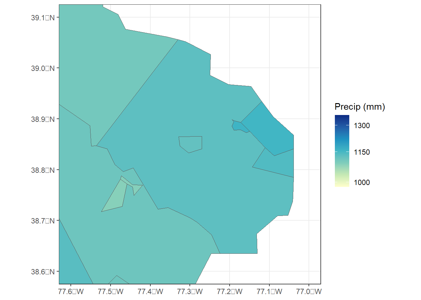
FIGURE 9.5: County-level zonal summaries of precipitation data from the PRISM dataset for northern Virginia using raster with 1 km cell size.
It should be noted that the PRISM climate data can also be downloaded at their native resolution of 800 m, and using these finer-resoluation data would be the best approach in real applications. The coarser 4 km dataset was used in this example to reduce the downloaded data volume and to illustrate the potential problems that can arise when there is a scale mismatch between two datasets.
There are other scale issues that should be taken into account when working with zonal statistics. As shown in the previous example, the sizes of U.S. counties vary tremendously. Independent cities in Virginia may encompass only a few square kilometers, and thus have a relatively homogeneous climate. In the western U.S., counties are much larger and more heterogeneous. For example, King County Washington covers thousands of square kilometers ranging from the coast to the crest of the Cascade Mountain Range. Most people live in the coastal regions in and around the city of Seattle, and zonal summaries across the entire county are not a precise metric of the climates that they experience. This is one aspect of the well-known Modifiable Areal Unit Problem (MAUP) in geography (Dark and Bram 2007). Before conducting a zonal analysis, it is important to carefully consider the sizes and spatial patterns of the zones and ensure that they are appropriate for the specific question at hand.
9.4 Extracting Raster Values with Point Data
In other situations, it is necessary to extract raster cell values associated with specific point locations. The following example will assess the accuracy of the monthly PRISM precipitation datasets for 2018 by comparing them with weather station data. These data were previously downloaded using the prism package and imported into the prism_prec_2018 dataset.
The PRISM data will be compared to monthly station data from the small Oklahoma mesonet data file, mesodata_small.csv, which was introduced in Chapter 2. The geographic coordinates of these stations also need to be imported separately from the geoinfo.csv file.
mesosm <- read_csv("mesodata_small.csv")
geo_coords <- read_csv("geoinfo.csv")
The data frame containing the geographic coordinates is converted to an sf object using st_as_sf(). The unique() function returns a vector of the station ID codes in the Mesonet dataset, and a new sf object containing only the point data for these stations is generated using the filter() function.
geo_coords <- st_as_sf(geo_coords,
                       coords = c("lon", "lat"))
mystations <- unique(mesosm$STID)
station_pts <- geo_coords %>%
  filter(stid %in% mystations)
The extract() function is used to obtain the raster data associated with each of the four points. First, the multilayer raster containing the precipitation data is assigned layer names. Since there is one layer for each month, we can use month.abb, a built-in R constant that contains vector of twelve abbreviations for the months of the year.
month.abb
##  [1] "Jan" "Feb" "Mar" "Apr" "May" "Jun" "Jul" "Aug" "Sep"
## [10] "Oct" "Nov" "Dec"
names(prism_prec_2018) <- month.abb
prism_samp <- extract(prism_prec_2018,
                      vect(station_pts),
                      factors = T,
                      df = T)
There are twelve layers in the prism_prec_2018 raster stack, one for each month. Therefore, the table generated by extract() has 48 values (4 stations x 12 months).
dim(prism_samp)
## [1]  4 13
glimpse(prism_samp)
## Rows: 4
## Columns: 13
## $ ID  <dbl> 1, 2, 3, 4
## $ Jan <dbl> 0.000, 82.706, 10.658, 7.660
## $ Feb <dbl> 1.464, 343.607, 104.995, 78.992
## $ Mar <dbl> 0.000, 128.251, 31.580, 13.819
## $ Apr <dbl> 32.591, 128.465, 38.255, 64.245
## $ May <dbl> 53.662, 140.197, 96.068, 124.110
## $ Jun <dbl> 129.731, 75.741, 81.546, 204.971
## $ Jul <dbl> 93.196, 93.599, 70.848, 88.683
## $ Aug <dbl> 46.675, 160.207, 56.496, 69.179
## $ Sep <dbl> 37.529, 140.801, 59.430, 153.339
## $ Oct <dbl> 98.560, 163.322, 101.636, 107.868
## $ Nov <dbl> 8.252, 112.287, 30.242, 13.804
## $ Dec <dbl> 57.315, 174.494, 86.176, 112.201
The prism_samp data frame is in wide format, with one row for each station and one column for each month of precipitation data plus an additional column that contains a numerical ID code. The mesosm data frame is in a long format, with one row for each combintation of station, month, and year. Before comparing the month precipitation values from the two data sources, they must be reformatted and combined into a single data frame. There are a number of steps in this process, but they can be coded concisely using a series of piped dplyr and tidyr functions as described in Chapter 3.
The bind_cols() function is used to add the columns of the original station location data frame, station_pts to prism_samp. This function only works if the two data frames have the same number of rows, and the columns of the second data frame are simply appended to the first. This step is necessary to add the station ID codes, which will be needed later.
The pivot_longer function is used to combine all twelve precipitation columns, Jan through Dec, into a new column called PPrec while the corresponding month abbreviations are stored in mnth_name.
The mutate() function adds two new columns: month contains numeric codes for each month that are generated with the match() function, and PPrec_in contains the PRISM precipitation values converted to inches.
The inner_join() function is used to join these data with mesosm, which contains the Mesonet data from the stations, by station ID code and month number.
Finally, the filter() function extracts only the 2018 records, and the select() function retains only the columns that are needed for subsequent graphing and analysis.
compare_prec <- prism_samp %>%
  bind_cols(station_pts) %>%
  pivot_longer(Jan:Dec,
               names_to = "mnth_name",
               values_to = "PPrec") %>%
  mutate(month = match(mnth_name, month.abb),
         PPrec_in = PPrec * 0.0393701) %>%
  inner_join(mesosm, by = c("stid" = "STID", "month" = "MONTH")) %>%
  filter(YEAR == 2018) %>%
  select(stid, month, RAIN, PPrec_in)
The critical variables in the resulting data frame are the monthly rainfall measured at the mesonet stations (RAIN) and the monthly rainfall estimates from the PRISM dataset converted to inches to match the Mesonet data (Pprec_in) along with the station ID (stid) and month (month) codes.
glimpse(compare_prec)
## Rows: 48
## Columns: 4
## $ stid     <chr> "HOOK", "HOOK", "HOOK", "HOOK", "HOOK", "…
## $ month    <dbl> 1, 2, 3, 4, 5, 6, 7, 8, 9, 10, 11, 12, 1,…
## $ RAIN     <dbl> 0.00, 0.06, 0.00, 1.25, 1.92, 5.07, 2.85,…
## $ PPrec_in <dbl> 0.00000000, 0.05763783, 0.00000000, 1.283…
The compare_prec data frame can now be used to generate a scatterplot showing the relationship between Mesonet weather station data on the x-axis and gridded PRISM data on the y-axis (Figure 9.6). The geom_abline() function is used to add a dashed 1:1 line to the graph. Of the four stations, Mt. Herman (MTHE) appears to have the largest deviations from the 1:1 line.
ggplot(data = compare_prec) +
  geom_point(aes(x = RAIN,
                 y = PPrec_in,
                 color = stid)) +
  scale_color_discrete(name = "Station ID") +
  geom_abline(slope = 1,
              intercept = 0,
              size = 0.25,
              linetype = "dashed") +
  xlab("Mesonet rainfall (in)") +
  ylab("PRISM rainfall (in)") +
  theme_bw()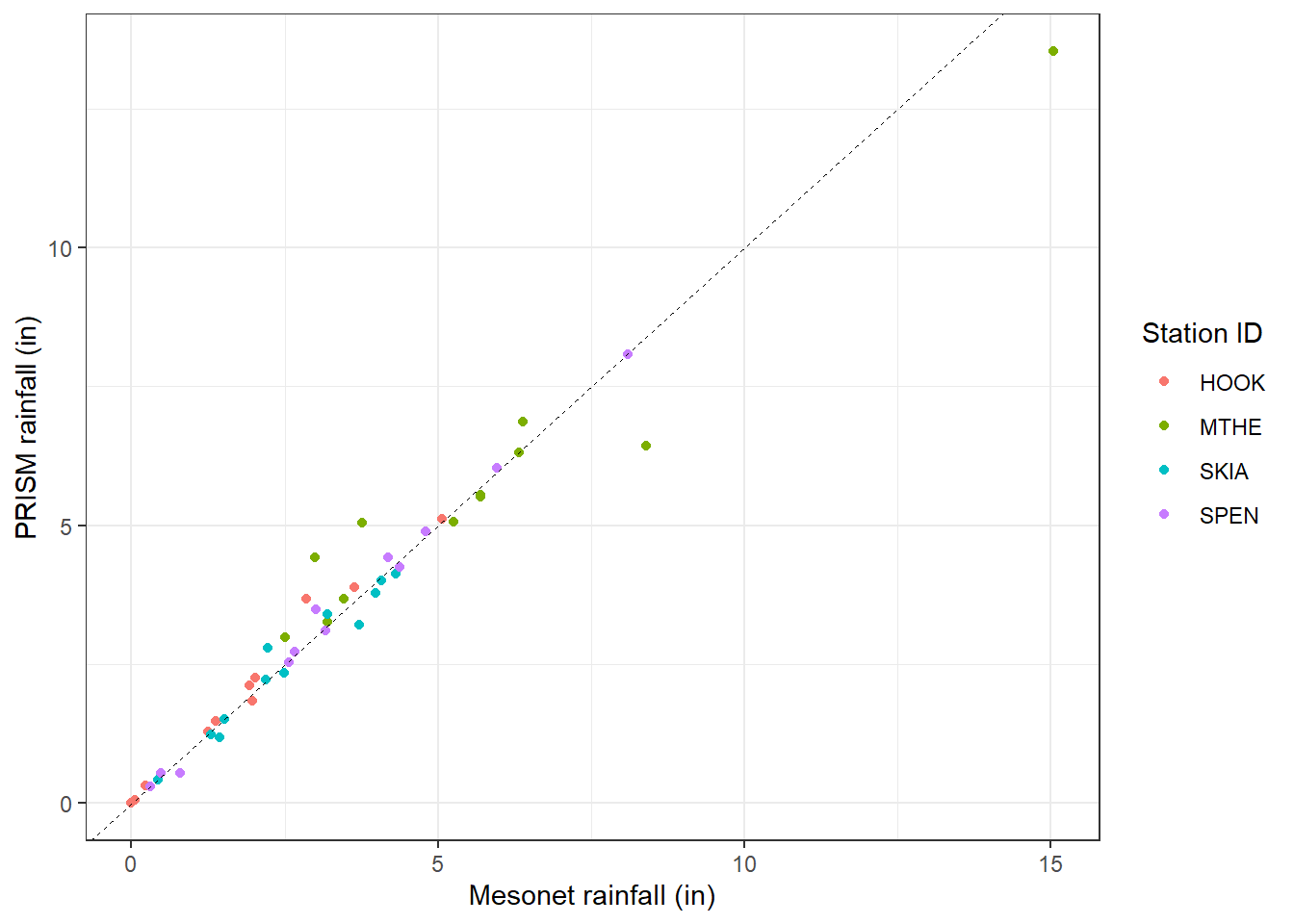
FIGURE 9.6: Scatterplot of monthly 2018 precipitation data from the Oklahoma Mesonet versus PRISM for four stations in Oklahoma.
The following code generates some additional summary statistics for the relationships between these precipitation estimates. The linear regression has a high R-squared and a slope that is only slightly less than one.
rain_lm <- lm(PPrec_in ~ RAIN, data = compare_prec)
summary(rain_lm)
##
## Call:
## lm(formula = PPrec_in ~ RAIN, data = compare_prec)
##
## Residuals:
##      Min       1Q   Median       3Q      Max
## -1.56891 -0.25019 -0.06633  0.20765  1.37211
##
## Coefficients:
##             Estimate Std. Error t value Pr(>|t|)
## (Intercept)  0.31273    0.10799   2.896  0.00577 **
## RAIN         0.91502    0.02528  36.196  < 2e-16 ***
## ---
## Signif. codes:
## 0 '***' 0.001 '**' 0.01 '*' 0.05 '.' 0.1 ' ' 1
##
## Residual standard error: 0.466 on 46 degrees of freedom
## Multiple R-squared:  0.9661, Adjusted R-squared:  0.9653
## F-statistic:  1310 on 1 and 46 DF,  p-value: < 2.2e-16
Other accuracy statistics such as the root mean squared error (RMSE), mean absolute error (MAE), and mean error (ME) are calculated using the summarize() function. These all have relatively low values, indicating a close agreement between the PRISM and Mesonet rainfall measurements.
rain_sum <- compare_prec %>%
  summarize(RMSE = sqrt(mean((PPrec_in - RAIN)^2)),
            MAE = mean(abs(PPrec_in - RAIN)),
            ME = mean(PPrec_in - RAIN))
rain_sum
## # A tibble: 1 × 3
##    RMSE   MAE     ME
##   <dbl> <dbl>  <dbl>
## 1 0.510 0.283 0.0287
There seems to be a very strong relationship between the two data sources. However, the Oklahoma Mesonet dataset is one of the sources of station data that are used to develop the interpolated PRISM dataset. So the two datasets are not entirely independent. Although the PRISM precipitation estimates are well calibrated to the Mesonet observations, this relationship may not be representative of PRISM accuracy at other locations where there are no Mesonet stations.
9.5 Practice
Starting with the
sfobject containing the county-level precipitation summaries, convert the precipitation units from millimeters to inches. Then classify precipitation into a factor with five categories: 0-10, 10-35, 35-50, 50-70, and > 70 inches. Generate a new map of precipitation using these categories.Generate a map of mean annual temperature summarized by county for the conterminous United States. You can access the PRISM mean temperature data by using
get_prism_normals()and specifyingtype = 'tmean'. Then you will need to recreate theprism_pathsvector and select the appropriate element to import the temperature raster. Compute zonal summaries of mean temperature for every county and create a map to display the results. The distribution of temperature is much less skewed than that of precipitation, so a logarithmic transformation is not needed.Repeat the comparison of gridded PRISM data and Mesonet station data using maximum temperature. You can access the PRISM maximum temperature data by using the
get_prism_monthly()and specifyingtype = 'tmax'. The corresponding variable in the Mesonet dataset isTMAX.