Chapter 10 Combining Vector Data with Discrete Raster Data
This chapter will introduce several new datasets and additional examples of integrating vector and raster data. The Cropland Data Layer (CDL) is a categorical raster dataset that maps agricultural land use in the United States. It provides annual data on locations where specific crop types such as corn, soybeans, wheat, and many others are planted. These maps are produced by the United States Department of Agriculture (USDA), which collects massive amounts of field-level data on planted crops from farmers. The data are used to train machine learning algorithms that predict the spatial pattern of crop types using satellite remote sensing data (Boryan et al. 2011). The CDL datasets can be visualized and accessed through the CropScape online platform (https://nassgeodata.gmu.edu/CropScape/).
The National Hydrography Dataset (NHD) contains vector data on the water drainage network in the United States. It consists of points, lines, and polygons that represent hydrological unit boundaries as well as features such as lakes, ponds, rivers, and streams. These data can be downloaded through the United State Geological Survey (USGS) National Map (https://apps.nationalmap.gov/downloader/).
This chapter will use downloaded data files characterizing crop types, hydrological unit boundaries, and stream data from the Middle Big Sioux Subbasin in eastern South Dakota. However, these data can also be accessed directly through R using the CropScapeR (Chen 2021) and nhdR (Stachelek 2022) packages.
Analyzing changes in the relative abundance of crop types and other land cover classes is important for understanding how agricultural land use is changing over time. In eastern South Dakota and other locations at the edge of the U.S. “Corn Belt”, there is concern that expanding cropland is reducing the cover of grasslands, including lands managed for pasture and hay as well as native prairie remnants (Michael C. Wimberly et al. 2017). Knowing whether these changes are occurring close to streams and other water bodies is important for assessing their impacts on wildlife habitat, carbon storage, and water quality.
The required R packages have all been used before with the exception of ggspatial (Dunnington 2022), which provides some additional functions for map annotations when using ggplot(). The rasterdf() function is also sourced for mapping the raster data in ggplot().
library(tidyverse)
library(sf)
library(terra)
library(scales)
library(colorspace)
library(ggspatial)
source("rasterdf.R")
The raster data include TIF files for 2010 and 2020 CDL data covering a portion of eastern South Dakota that were downloaded using the CropScape website. The vector data include shapefiles with flowlines, watershed boundaries, and subwatershed boundaries within the Middle Big Sioux subbasin in eastern South Dakota.
# Read in the data
crop2010 <- rast("CDL_2010_clip.tif")
crop2020 <- rast("CDL_2020_clip.tif")
streams <- st_read("NHDFlowline.shp", quiet = TRUE)
wsheds <- st_read("WBDHU10.shp", quiet = TRUE)
subwsh <- st_read("WBDHU12.shp", quiet = TRUE)
Before trying to combine the two data sources, it is important to check their coordinate reference systems. The NHD data are in a geographic coordinate system.
writeLines(st_crs(wsheds)$WktPretty)
## GEOGCS["NAD83",
##     DATUM["North_American_Datum_1983",
##         SPHEROID["GRS 1980",6378137,298.257222101]],
##     PRIMEM["Greenwich",0],
##     UNIT["degree",0.0174532925199433,
##         AUTHORITY["EPSG","9122"]],
##     AXIS["Latitude",NORTH],
##     AXIS["Longitude",EAST],
##     AUTHORITY["EPSG","4269"]]
The CDL data are in a projected Albers Equal Area coordinate system.
writeLines(st_crs(crop2010)$WktPretty)
## PROJCS["unnamed",
##     GEOGCS["NAD83",
##         DATUM["North_American_Datum_1983",
##             SPHEROID["GRS 1980",6378137,298.257222101004]],
##         PRIMEM["Greenwich",0],
##         UNIT["degree",0.0174532925199433,
##             AUTHORITY["EPSG","9122"]],
##         AUTHORITY["EPSG","4269"]],
##     PROJECTION["Albers_Conic_Equal_Area"],
##     PARAMETER["latitude_of_center",23],
##     PARAMETER["longitude_of_center",-96],
##     PARAMETER["standard_parallel_1",29.5],
##     PARAMETER["standard_parallel_2",45.5],
##     PARAMETER["false_easting",0],
##     PARAMETER["false_northing",0],
##     UNIT["metre",1,
##         AUTHORITY["EPSG","9001"]],
##     AXIS["Easting",EAST],
##     AXIS["Northing",NORTH]]
For the reasons discussed in Chapter 8, all three vector datasets are reprojected to match the coordinate system of the raster data rather than reprojecting the raster data.
wsheds_aea <- st_transform(wsheds, crs(crop2010))
subwsh_aea <- st_transform(subwsh, crs(crop2010))
streams_aea <- st_transform(streams, crs(crop2010))
10.1 Visualizing and Manipulating Vector Data
The first step is to explore the watersheds within the Middle Big Sioux Subbasin by generating a labeled map. First, columns with x and y coordinates are added to the wsheds object to make it possible to label the watersheds. For map labels, it is advisable to use st_point_on_surface() instead of st_centroid() to ensure that the label points fall inside the polygons. The st_coordinates() function converts these coordinates into a geometry column that can be interpreted by sf functions. Then a labeled map of watersheds is generated by using geom_sf() to plot the watershed boundaries (the default fill color is gray) and using geom_text() to write the name of each watershed at its label point (Figure 10.1).
wsheds_aea <- cbind(wsheds_aea,
                    st_coordinates(st_point_on_surface(wsheds_aea)))

ggplot(data = wsheds_aea) +
  geom_sf(color = "black",
          size = 0.1) +
  geom_text(aes(x = X,
                y = Y,
                label = name),
            size = 3,
            fontface = "bold") +
  coord_sf() +
  theme_void()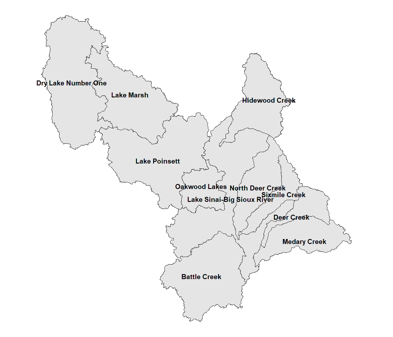
FIGURE 10.1: Watersheds in the Middle Big Sioux subbasin.
Some of the labels are crowded and difficult to read. Also, because of the complex shapes of some of the watersheds, the point locations generated by st_point_on_surface() are not well centered. When there are relatively few labels as in this example, it is often possible to adjust the text placement manually. This is the order of watersheds in the wsheds data frame.
wsheds$name
##  [1] "Lake Sinai-Big Sioux River"
##  [2] "Deer Creek"
##  [3] "Medary Creek"
##  [4] "Dry Lake Number One"
##  [5] "Lake Marsh"
##  [6] "Lake Poinsett"
##  [7] "Hidewood Creek"
##  [8] "Oakwood Lakes"
##  [9] "Sixmile Creek"
## [10] "North Deer Creek"
## [11] "Battle Creek"
The following code adjusts the text positions for “Lake Sinai-Big Sioux River” (position 1), “Deer Creek (position 2), and North Deer Creek (position 10). The hnudge and vnudge vectors contain the horizontal and vertical adjustments for all eleven watersheds. These values are in map units, which in this case are meters. Zero values are provided when the positions will not be adjusted. Then, the nudge_x = hnudge and nudge_y = vnudge arguments to geom_text() are specified when generating the map text. Further refinements could be made, but the text here is at least a bit more readable. (Figure 10.2).
hnudge <- c(-10000, 5000, 0, 0, 0, 0, 0, 0, 0, 0, 0)
vnudge <- c(-7500, 2500, 0, 0, 0, 0, 0, 0, 0, 5000, 0)

ggplot(data = wsheds_aea) +
  geom_sf(color = "black",
          size = 0.1) +
  geom_text(aes(x = X,
                y = Y,
                label = name),
            nudge_x = hnudge,
            nudge_y = vnudge,
            size = 3,
            fontface = "bold") +
  theme_void()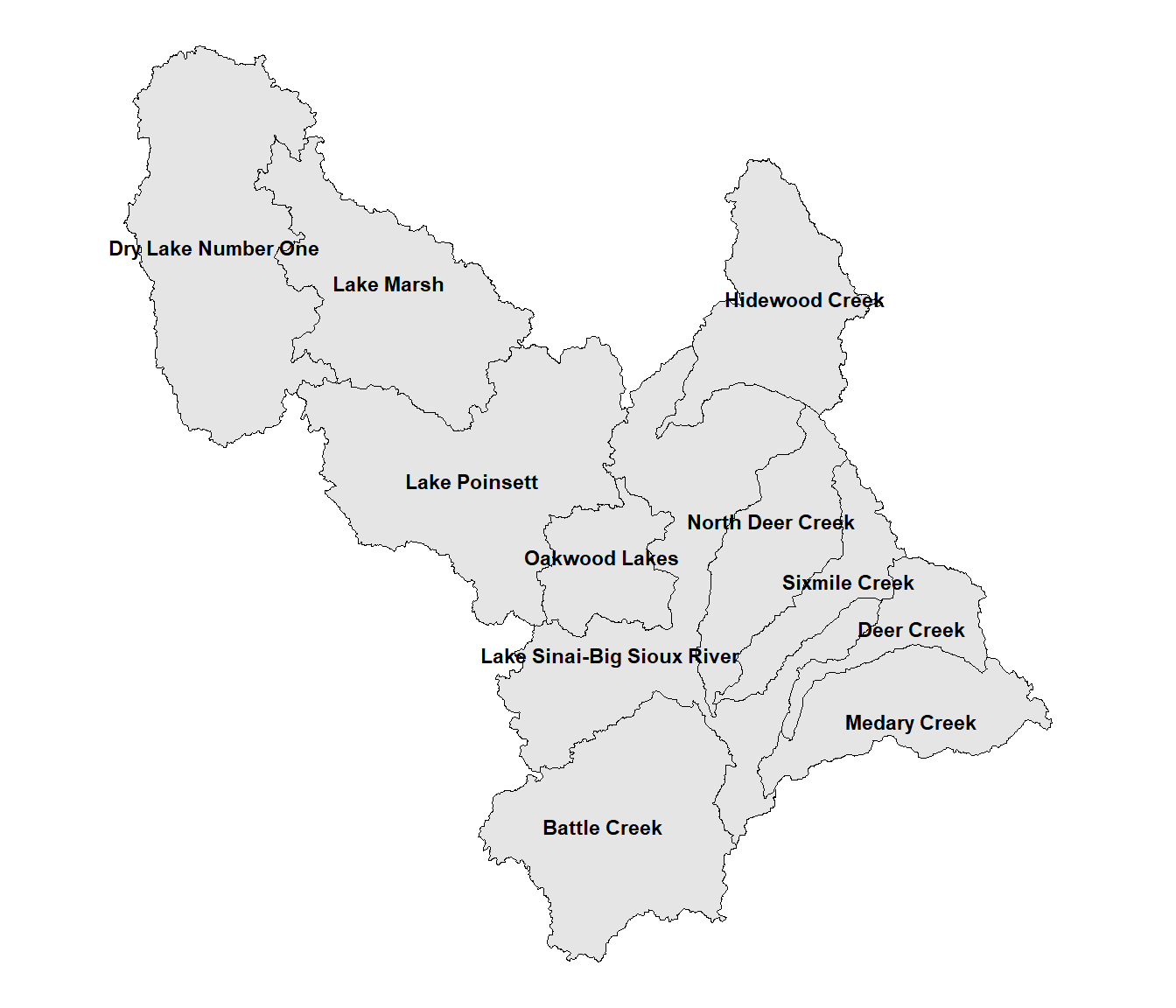
FIGURE 10.2: Watersheds in the Middle Big Sioux subbasin with manually adjusted label positions.
The label positions can also be modified using an alternative geom function. The geom_spatial_label_repel() function from the ggspatial package automatically modifies the label placement to keep them from overlapping (Figure 10.3). The argument label = str_wrap(name, 15) forces the labels to wrap so that the maximum width is 15 characters, which makes them more compact.
ggplot(data = wsheds_aea) +
  geom_sf(color = "black",
          size = 0.1) +
  geom_spatial_label_repel(aes(x = X,
                               y = Y,
                               label = str_wrap(name, 15)),
                           size = 3,
                           fontface = "bold",
                           crs = st_crs(wsheds_aea)) +
  theme_void()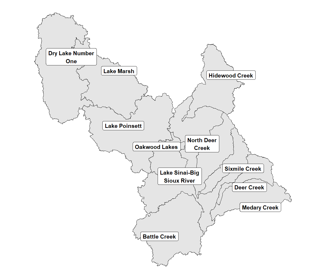
FIGURE 10.3: Watersheds in the Middle Big Sioux subbasin with automatically adjusted label positions.
The next map includes the watershed boundaries as well as the nested subwatershed boundaries displayed in dark gray (Figure 10.4). Because the data are from multiple data frames, the data argument needs to be included in the geom_sf() functions instead of the initial ggplot() function. The annotation_scale() function from the ggspatial package is also used to add a scale bar to better discern the sizes of the polygons.
ggplot() +
  geom_sf(data = subwsh_aea, color = "darkgray") +
  geom_sf(data = wsheds_aea, color = "black", fill = NA) +
  annotation_scale(location = 'bl') +
  theme_void()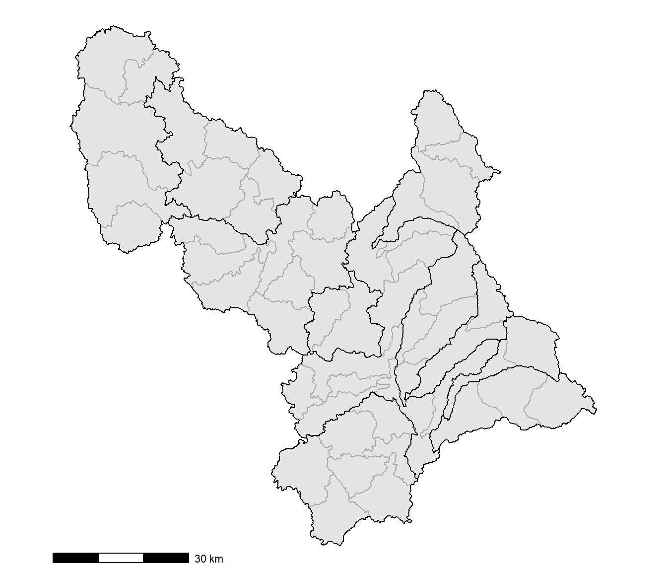
FIGURE 10.4: Watersheds and subwatersheds in the Middle Big Sioux subbasin.
The following analyses will focus on the North Deer Creek watershed. To extract the boundary for only this watershed, the filter() function is used.
wshed_ndc <- wsheds_aea %>%
  filter(name == "North Deer Creek")
A second filter() function with a nested sf_covered_by() function is then used to make a spatial query that selects all subwatershed polygons in the subwsh_aea layer that fall within the North Deer Creek watershed.
subwsh_ndc <- subwsh_aea %>%
  filter(lengths(st_covered_by(., wshed_ndc)) > 0)
10.2 Zonal Summaries of Discrete Raster Data
To summarize the crop type data for each subwatershed, the CDL data are first cropped and masked to the boundaries of the North Deer Creek watershed.
cdlstack <- c(crop2010, crop2020)
names(cdlstack) <- c("2010", "2020")

cdl_crop <- crop(cdlstack, vect(subwsh_ndc))
subwsh_msk <- rasterize(vect(subwsh_ndc), cdl_crop)
cdl_mbs <- mask(cdl_crop, subwsh_msk)
The approach that was introduced in Chapter 7 is used to reclassify the CDL into a smaller number of classes. The most widespread crops in this region are corn (1) and soybeans (5). Grasslands and pastures (37) non-alfalfa hay (176) and herbaceous wetlands (195) are combined into a single grass class. The others = 4 argument in the classify() function is used to combine all the other codes into a single class.
oldclas <- c(1, 5, 37, 176, 195)
newclas <- c(1, 2, 3, 3, 3)
lookup <- data.frame(oldclas, newclas)
cdl_rc <- classify(cdl_mbs,
                       rcl = lookup,
                       others = 4)
The reclassified rasters are then plotted with the subwatershed boundaries overlaid (Figure 10.5).
newnames <- c("Corn",
              "Soybeans",
              "Grass",
              "Other")
newcols <- c("yellow",
             "green",
             "tan",
             "gray60")
newcols2 <- desaturate(newcols,
                       amount = 0.2)
cdl_df <- rasterdf(cdl_rc)

ggplot(data = cdl_df) +
  geom_raster(aes(x = x,
                  y = y,
                  fill =
                    as.character(value))) +
  scale_fill_manual(name = "Crop Type",
                    values = newcols2,
                    labels = newnames,
                    na.translate = FALSE) +
  geom_sf(data = subwsh_ndc,
          fill = NA) +
  facet_wrap(facets = vars(variable), ncol = 2) +
  theme_void() +
  theme(strip.text.x = element_text(size=12, face="bold"))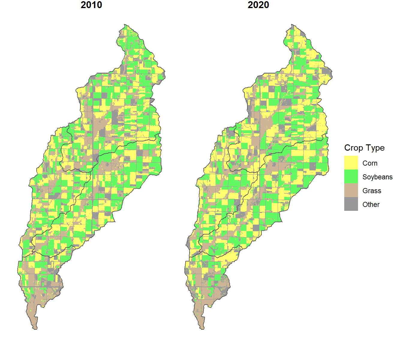
FIGURE 10.5: Subwatershed boundaries overlaid on the cropland data layer in the North Deer Creek watershed
The zonal() function, introduced in Chapter 9, is useful for generating statistical summaries of continuous data. However, a different approach is needed to summarize discrete data, where we want to estimate the areas of different classes within each polygon. We start by rasterizing the subwatershed polygons to match the raster grid of the land cover data. Then the crosstab() function, which was used for change analysis in Chapter 7, is used to calculate the number of cells of each land cover type within each subwatershed polygon.
subwsh_r <- rasterize(vect(subwsh_ndc),
                      cdl_rc,
                      field = "ObjectID")
cdlsum10 <- crosstab(c(subwsh_r, cdl_rc[["2010"]]))
cdlsum10 <- as_tibble(cdlsum10)
cdlsum20 <- crosstab(c(subwsh_r, cdl_rc[["2020"]]))
cdlsum20 <- as_tibble(cdlsum20)
Next, a series of dplyr() and tidyr() commands are used to convert the crosstabulation results into a long format for mapping and then compute the percent area of each crop type in each subwatershed. The process will be broken down into multiple steps.
The inner_join() function is used to join the 2010 and 2020 crosstabulation results by the subwatershed code (stored in ObjectID) and the crop type code (stored in X2010 and X2020).
cdljoin <- cdlsum10 %>%
  inner_join(cdlsum20,
             by = c("ObjectID" = "ObjectID",
                    "X2010" = "X2020"))
cdljoin
## # A tibble: 16 × 4
##    ObjectID X2010   n.x   n.y
##    <chr>    <chr> <int> <int>
##  1 38       1     42810 53551
##  2 39       1     22745 26070
##  3 40       1     35535 37192
##  4 41       1      6603  8636
##  5 38       2     48192 43019
##  6 39       2     22238 19146
##  7 40       2     40287 41062
##  8 41       2      8704  6928
##  9 38       3     32396 25490
## 10 39       3     13584 12382
## 11 40       3     19865 16614
## 12 41       3     17892 16703
## 13 38       4     21846 23184
## 14 39       4      7172  8141
## 15 40       4     13298 14117
## 16 41       4      7155  8087
The resulting table has the crop type codes stored in the X2010 column. The mutate() function is used to convert these to a new croptype column that is a factor with labels for each of the crop type names. The old X2010 column is discarded. New names are assigned to the n.x and n.y columns, which contain the counts of the 2010 and 2020 crop types for each subwatershed.
cdljoin2 <- cdljoin %>%
  mutate(croptype = factor(X2010,
                           labels = newnames),
         ObjectID = as.numeric(ObjectID)) %>%
  select(-X2010) %>%
  rename("cnt2010" = "n.x",
         "cnt2020" = "n.y")
cdljoin2
## # A tibble: 16 × 4
##    ObjectID cnt2010 cnt2020 croptype
##       <dbl>   <int>   <int> <fct>
##  1       38   42810   53551 Corn
##  2       39   22745   26070 Corn
##  3       40   35535   37192 Corn
##  4       41    6603    8636 Corn
##  5       38   48192   43019 Soybeans
##  6       39   22238   19146 Soybeans
##  7       40   40287   41062 Soybeans
##  8       41    8704    6928 Soybeans
##  9       38   32396   25490 Grass
## 10       39   13584   12382 Grass
## 11       40   19865   16614 Grass
## 12       41   17892   16703 Grass
## 13       38   21846   23184 Other
## 14       39    7172    8141 Other
## 15       40   13298   14117 Other
## 16       41    7155    8087 Other
The pivot_longer() function is used to combine the 2010 and 2020 cell counts into a single cnt column with year information stored in the year column. The parse_number() function is then used to convert year from a character to a number.
cdlpivot <- cdljoin2 %>%
  pivot_longer(cols = starts_with("cnt"),
               names_to = "year",
               values_to = "cnt") %>%
  mutate(year = parse_number(year))
cdlpivot
## # A tibble: 32 × 4
##    ObjectID croptype  year   cnt
##       <dbl> <fct>    <dbl> <int>
##  1       38 Corn      2010 42810
##  2       38 Corn      2020 53551
##  3       39 Corn      2010 22745
##  4       39 Corn      2020 26070
##  5       40 Corn      2010 35535
##  6       40 Corn      2020 37192
##  7       41 Corn      2010  6603
##  8       41 Corn      2020  8636
##  9       38 Soybeans  2010 48192
## 10       38 Soybeans  2020 43019
## # … with 22 more rows
The total number of pixels for each combination of subwatershed and year is summed, and the percent area of each crop type within each subwatershed is calculated.
cdlperc <- cdlpivot %>%
  group_by(ObjectID, year) %>%
  mutate(tot = sum(cnt),
         perc_crop = 100 * cnt / tot)
cdlperc
## # A tibble: 32 × 6
## # Groups:   ObjectID, year [8]
##    ObjectID croptype  year   cnt    tot perc_crop
##       <dbl> <fct>    <dbl> <int>  <int>     <dbl>
##  1       38 Corn      2010 42810 145244      29.5
##  2       38 Corn      2020 53551 145244      36.9
##  3       39 Corn      2010 22745  65739      34.6
##  4       39 Corn      2020 26070  65739      39.7
##  5       40 Corn      2010 35535 108985      32.6
##  6       40 Corn      2020 37192 108985      34.1
##  7       41 Corn      2010  6603  40354      16.4
##  8       41 Corn      2020  8636  40354      21.4
##  9       38 Soybeans  2010 48192 145244      33.2
## 10       38 Soybeans  2020 43019 145244      29.6
## # … with 22 more rows
Note that the same code can also be implemented more concisely as a single block of piped functions.
cdlperc <- cdlsum10 %>%
  inner_join(cdlsum20,
             by = c("ObjectID" = "ObjectID",
                    "X2010" = "X2020")) %>%
  mutate(croptype = factor(X2010,
                           labels = newnames),
         ObjectID = as.numeric(ObjectID)) %>%
  rename("cnt2010" = "n.x",
         "cnt2020" = "n.y") %>%
  pivot_longer(cols = starts_with("cnt"),
               names_to = "year",
               values_to = "cnt") %>%
  mutate(year = parse_number(year)) %>%
  group_by(ObjectID, year) %>%
  mutate(tot = sum(cnt),
         perc_crop = 100 * cnt / tot)
The resulting table can be joined to the data frame containing the subwatershed polygons and used to map the percent of each crop type by subwatershed in 2010 and 2020 (Figure 10.6). The facet_wrap() function with the formula year ~ croptype is used to create a layout with years as rows and crop types as columns.
subwsh_perc <- left_join(subwsh_ndc,
                         cdlperc,
                         by = "ObjectID")

ggplot(data = subwsh_perc) +
  geom_sf(aes(fill = perc_crop)) +
  scale_fill_distiller(name="Percent",
                       palette = "YlGn",
                       breaks = pretty_breaks(),
                       direction = 1) +
  facet_wrap(year ~ croptype,
             ncol = 4) +
  theme_void() +
  theme(strip.text.x = element_text(size=12, face="bold"))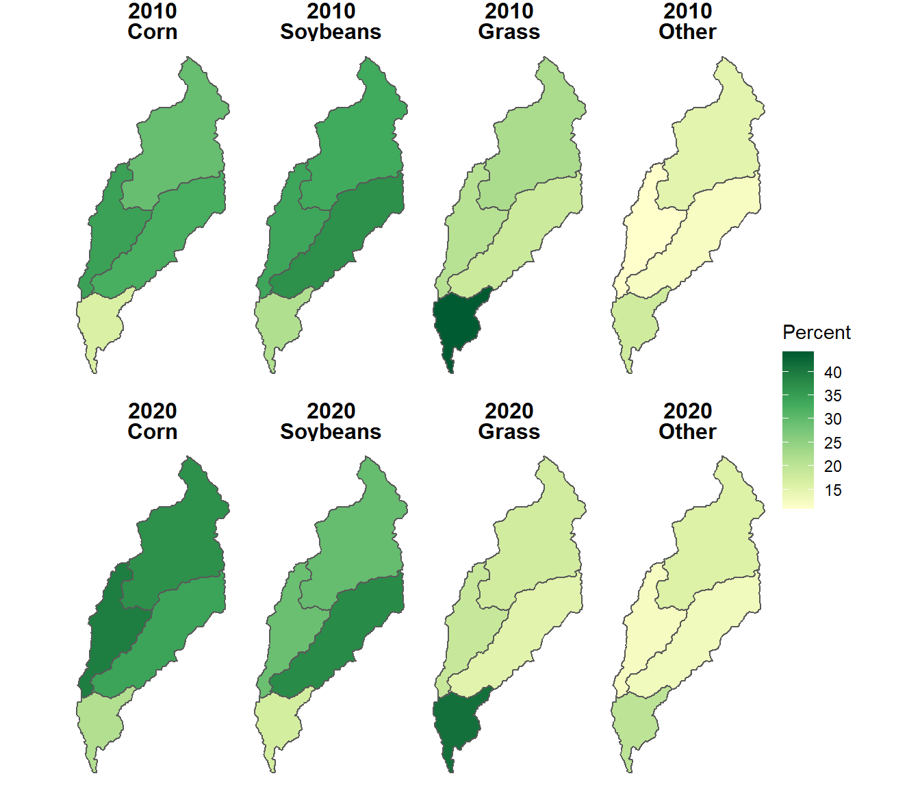
FIGURE 10.6: Proportional area of each crop type summarized by subwatershed in the North Deer Creek watershed.
10.3 Summarizing Land Cover With Stream Buffers
The stream lines from the NHD are read in as three-dimensional data with Z coordinates, and they need to be converted to two-dimensional data before we can work with them. This step is accomplished using the st_zm() function. The st_intersection() function is then used to clip the streams to the North Deer Creek watershed boundary, and the result is plotted (Figure 10.7).
streams_aea <- st_zm(streams_aea)
streams_ndc <- st_intersection(streams_aea, wshed_ndc)

ggplot() +
  geom_sf(data = subwsh_ndc,
          color = "black",
          size = 1) +
  geom_sf(data = streams_ndc,
          color = "blue") +
  theme_void()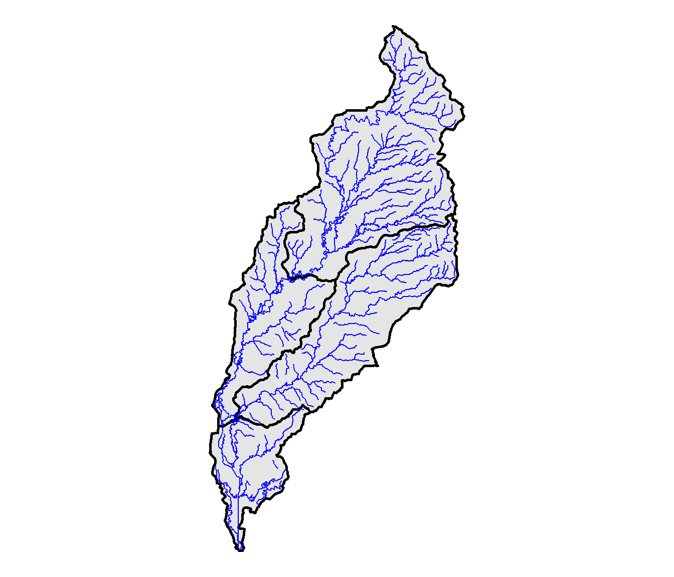
FIGURE 10.7: NHD streams in the North Deer Creek watershed.
Stream buffers are computed with the st_buffer() function. The dist argument provides the buffer width in map units, which in this case are meters. The output contains a separate buffer polygon for each line segment in the stream network (Figure 10.8).
streams_buff <- st_buffer(streams_ndc, dist = 100)

ggplot() +
  geom_sf(data = wshed_ndc,
          color = "black",
          size = 1) +
  geom_sf(data = streams_buff,
          color = "blue") +
  theme_void()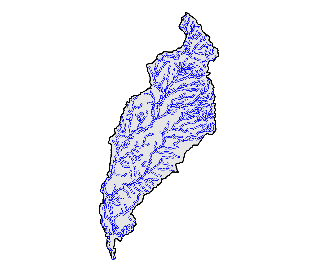
FIGURE 10.8: Buffers for each stream segment in the North Deer Creek watershed.
The st_union() function is used to combine the separate buffer polygons into a single polygon. Note that st_union() creates a simple feature geometry list column (sfc) that needs to be converted into an an sf object before undertaking further analysis.
streams_comb <- st_union(streams_buff)
class(streams_comb)
## [1] "sfc_MULTIPOLYGON" "sfc"
streams_comb <- st_sf(streams_comb)
class(streams_comb)
## [1] "sf"         "data.frame"
Where streams are close to the watershed boundary, their buffers may extend outside of the watershed. The st_intersection() function combines the stream buffers with the North Deer Creek watershed polygon to create a polygon encompassing all stream buffers inside the watershed. The st_difference() function similarly creates a polygon encompassing the parts of the North Deer Creek watershed that are outside the stream buffers.
riparian <- st_intersection(streams_comb, wshed_ndc)
upland <- st_difference(wshed_ndc, streams_comb)
The stream buffers can be mapped as polygon boundaries overlaid on top of the reclassified land cover dataset (Figure 10.9).
ggplot(data = cdl_df) +
  geom_raster(aes(x = x,
                  y = y,
                  fill = as.character(value))) +
  scale_fill_manual(name = "Land cover",
                    values = newcols2,
                    labels = newnames,
                    na.translate = FALSE) +
  facet_wrap(facets = vars(variable), ncol = 2) +
  geom_sf(data = streams_comb,
          color = "darkblue",
          fill = NA) +
  coord_sf(expand = F) +
  theme_void() +
  theme(strip.text.x = element_text(size=12, face="bold"))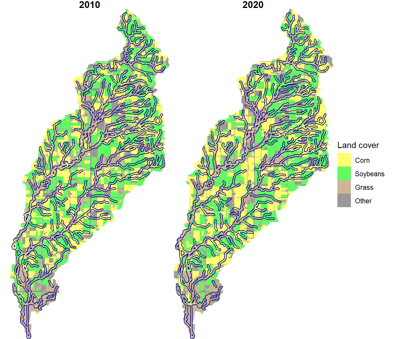
FIGURE 10.9: Stream buffers overlaid on crop types for the North Deer Creek watershed.
Two new raster datasets are created by masking the CDL dataset with the riparian and upland vector datasets.
riparian_mask <- rasterize(vect(riparian), cdl_rc)
cdl_rip <- mask(cdl_rc, riparian_mask)
upland_mask <- rasterize(vect(upland), cdl_rc)
cdl_up <- mask(cdl_rc, upland_mask)
The freq() function is used to compute the pixel counts in the resulting riparian and upland raster datasets.
freq_rip <- as_tibble(freq(cdl_rip))
freq_rip
## # A tibble: 8 × 3
##   layer value count
##   <dbl> <dbl> <dbl>
## 1     1     1 26599
## 2     1     2 26396
## 3     1     3 45230
## 4     1     4 12117
## 5     2     1 29395
## 6     2     2 24737
## 7     2     3 40868
## 8     2     4 15342
freq_up <- as_tibble(freq(cdl_up))
freq_up
## # A tibble: 8 × 3
##   layer value count
##   <dbl> <dbl> <dbl>
## 1     1     1 81094
## 2     1     2 93025
## 3     1     3 38507
## 4     1     4 37354
## 5     2     1 96054
## 6     2     2 85418
## 7     2     3 30321
## 8     2     4 38187
The outputs are combined using bind_rows() into a single data frame that contains pixel counts for each land cover class for the buffer and upland zones. This function will only work if the two data frames have the exact same column specifications, and it “stacks” them on top of one another. The landtype column is created to identify the riparian and upland records, and the year and croptype columns are derived from the layer and value columns output by the freq() function.
The pixel counts are used to calculate the percent cover for each subwatershed. First, the data are grouped by landtype (stream buffer versus upland), and then the mutate() function is run on the grouped data. Note that the results are different from the summarize() function. The mutate() function replicates the results of a summary (in this case, the sum() function) for each record within a group rather than returning a single value for each group. Having the grouped total of pixel counts on each line makes it straightforward to calculate the percent cover of each class.
cdl_chng <- freq_rip %>%
  bind_rows(freq_up) %>%
  mutate(landtype = c(rep("Riparian", 8), rep("Upland", 8)),
         year = factor(layer,
                       labels = c("2010", "2020")),
         croptype = factor(value,
                           labels = newnames)) %>%
  select(-layer, -value) %>%
  group_by(landtype) %>%
  mutate(totarea = sum(count),
         percarea = 100 * count / totarea)
cdl_chng
## # A tibble: 16 × 6
## # Groups:   landtype [2]
##    count landtype year  croptype totarea percarea
##    <dbl> <chr>    <fct> <fct>      <dbl>    <dbl>
##  1 26599 Riparian 2010  Corn      220684    12.1
##  2 26396 Riparian 2010  Soybeans  220684    12.0
##  3 45230 Riparian 2010  Grass     220684    20.5
##  4 12117 Riparian 2010  Other     220684     5.49
##  5 29395 Riparian 2020  Corn      220684    13.3
##  6 24737 Riparian 2020  Soybeans  220684    11.2
##  7 40868 Riparian 2020  Grass     220684    18.5
##  8 15342 Riparian 2020  Other     220684     6.95
##  9 81094 Upland   2010  Corn      499960    16.2
## 10 93025 Upland   2010  Soybeans  499960    18.6
## 11 38507 Upland   2010  Grass     499960     7.70
## 12 37354 Upland   2010  Other     499960     7.47
## 13 96054 Upland   2020  Corn      499960    19.2
## 14 85418 Upland   2020  Soybeans  499960    17.1
## 15 30321 Upland   2020  Grass     499960     6.06
## 16 38187 Upland   2020  Other     499960     7.64
These data can be graphed as a barchart to compare the distribution of crop types by year and by riparian or upland landscape zone (Figure 10.10). Riparian areas have more grass cover relative to corn and soybeans than upland areas. However, the area of grass cover has decreased in both riparian and upland areas between 2010 and 2020.
ggplot(data = cdl_chng) +
  geom_bar(aes(y = percarea,
               x = year,
               fill = croptype),
           color = "black",
           position = "dodge",
           stat = "identity")  +
  scale_fill_manual(name = "Land Cover",
                    values = newcols) +
  facet_wrap(facets = vars(landtype),
             ncol = 2) +
  labs(x = "Landscape Zone",
       y = "% Area") +
  theme_bw()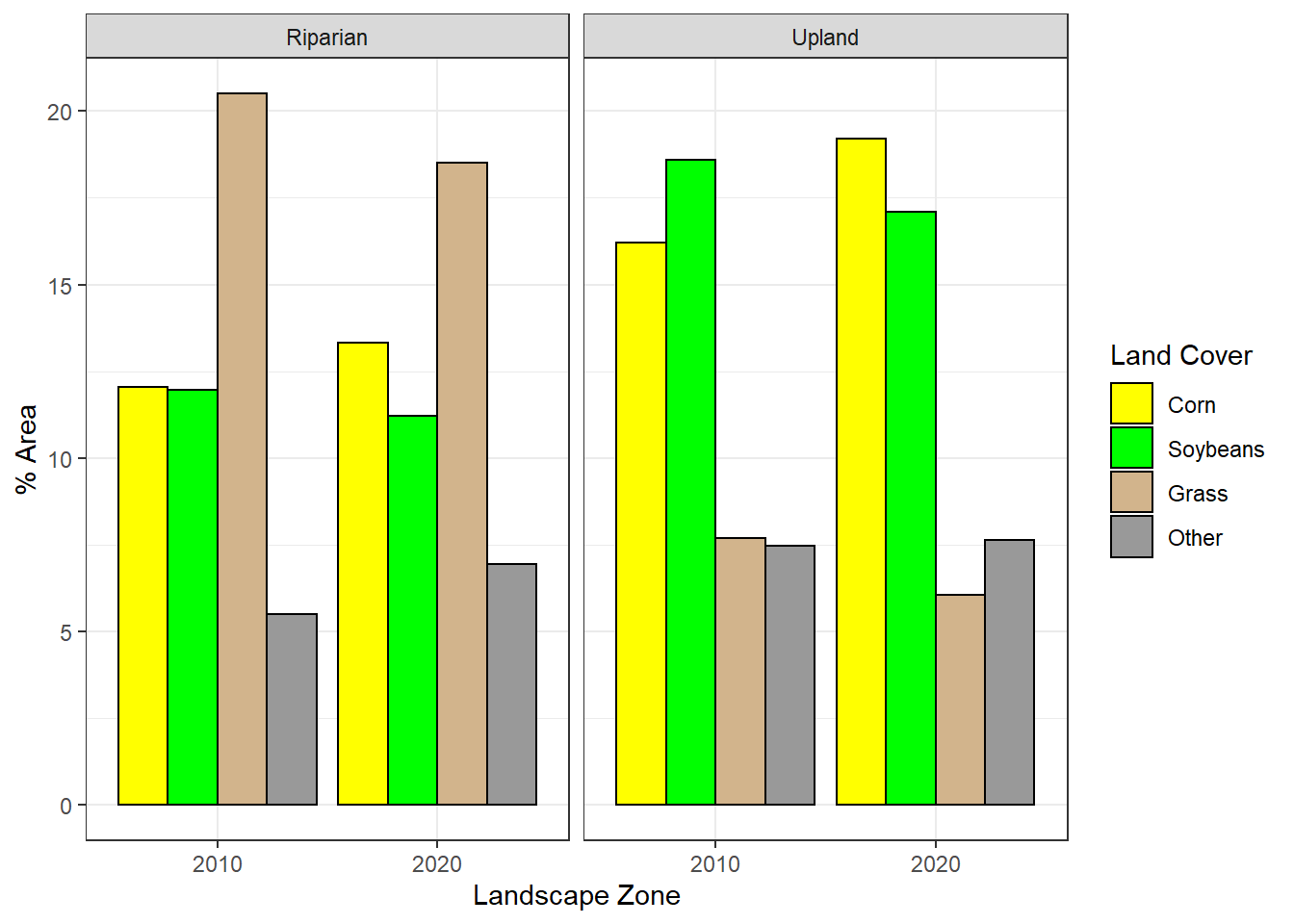
FIGURE 10.10: Areal distribution of crop types by landscape zone (riparian versus upland) and year.
10.4 Summarizing Land Cover With Point Buffers
For this example, a set of twenty random points is generated within the North Deer Creek watershed. These could represent vegetation plots, wildlife sampling points, or the locations of other field-based measurements. Like the st_buffer() function, st_sample() generates an sfc object that must be converted to an sf object.
set.seed(32145)
plots <- st_sample(wshed_ndc, size = 20)
class(plots)
## [1] "sfc_POINT" "sfc"
plots <- st_as_sf(plots)
class(plots)
## [1] "sf"         "data.frame"
The st_sample() function uses a random number generator to produce x and y coordinates for the plot locations. The set.seed() function provides a starting seed for the random number generator so that it will produce the same results every time the code is run. If no random number seed is provided, it is derived from the current time in the computer’s clock, and the results will be different every time the code is run.
The locations of these plots are plotted on top of the crop type data (Figure 10.11).
ggplot(data = cdl_df) +
  geom_raster(aes(x = x, y = y, fill = as.character(value))) +
  scale_fill_manual(name = "Land cover",
                    values = newcols2,
                    labels = newnames,
                    na.translate = FALSE) +
  geom_sf(data = plots, fill = NA) +
  facet_wrap(facets = vars(variable)) +
  coord_sf(expand = F) +
  theme_void() +
  theme(strip.text.x = element_text(size=12, face="bold"))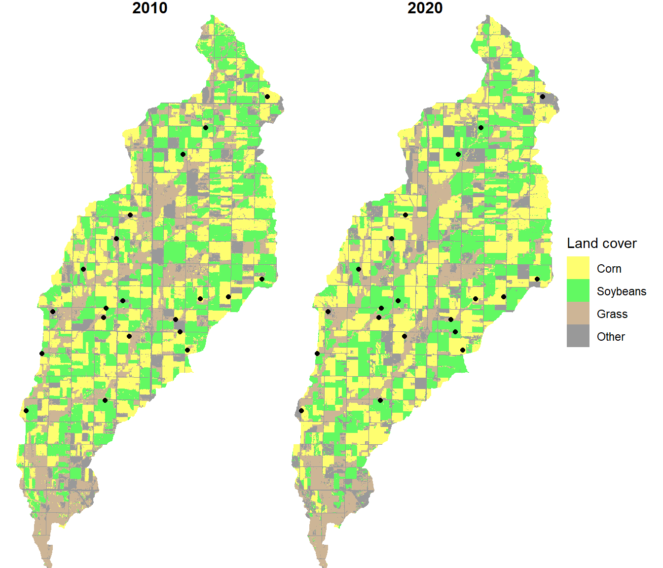
FIGURE 10.11: Plot locations overlaid on the crop type maps.
To summarize the percent cover of each land cover class within a buffer around each point, buffer polygons are created with a 200 m radius around each point.
st_geometry_type(plots, by_geometry = FALSE)
## [1] POINT
## 18 Levels: GEOMETRY POINT LINESTRING POLYGON ... TRIANGLE
plot_poly <- st_buffer(plots, dist = 200)
st_geometry_type(plot_poly, by_geometry = FALSE)
## [1] POLYGON
## 18 Levels: GEOMETRY POINT LINESTRING POLYGON ... TRIANGLE
To summarize the percent cover of each land cover class within a buffer around each point, the segregate() function is used to convert the classified raster data into a stack of indicator (1, 0) rasters. The proportion of each crop type within each buffer is computed using the extract() function with the fun = mean argument.
cdl_stk <- segregate(cdl_rc[["2020"]])
names(cdl_stk) <- newnames

plots_cdl <- extract(cdl_stk,
                    vect(plot_poly ),
                    fun = mean,
                    na.rm = T)
The resulting data frame has one row for each plot and one column for each crop type.
plots_cdl
##    ID        Corn   Soybeans      Grass       Other
## 1   1 1.000000000 0.00000000 0.00000000 0.000000000
## 2   2 0.000000000 1.00000000 0.00000000 0.000000000
## 3   3 0.582733813 0.00000000 0.10791367 0.309352518
## 4   4 0.425531915 0.04255319 0.31914894 0.212765957
## 5   5 0.028571429 0.52142857 0.43571429 0.014285714
## 6   6 0.042857143 0.81428571 0.04285714 0.100000000
## 7   7 0.944055944 0.00000000 0.02797203 0.027972028
## 8   8 0.021276596 0.68085106 0.18439716 0.113475177
## 9   9 0.728571429 0.23571429 0.00000000 0.035714286
## 10 10 0.000000000 0.00000000 0.44927536 0.550724638
## 11 11 0.228571429 0.01428571 0.75000000 0.007142857
## 12 12 0.007142857 0.00000000 0.00000000 0.992857143
## 13 13 0.223076923 0.13076923 0.50000000 0.146153846
## 14 14 0.453237410 0.29496403 0.03597122 0.215827338
## 15 15 0.214285714 0.30000000 0.47142857 0.014285714
## 16 16 0.014285714 0.92857143 0.00000000 0.057142857
## 17 17 0.471014493 0.03623188 0.31159420 0.181159420
## 18 18 0.000000000 1.00000000 0.00000000 0.000000000
## 19 19 0.000000000 0.90647482 0.00000000 0.093525180
## 20 20 0.421428571 0.08571429 0.28571429 0.207142857
It is converted to a long format with all the crop type proportions in a single column and crop type names in a separate column.
plots_long <- plots_cdl %>%
  pivot_longer(Corn:Other,
               names_to = "croptype",
               values_to = "percarea")
plots_long
## # A tibble: 80 × 3
##       ID croptype percarea
##    <dbl> <chr>       <dbl>
##  1     1 Corn        1
##  2     1 Soybeans    0
##  3     1 Grass       0
##  4     1 Other       0
##  5     2 Corn        0
##  6     2 Soybeans    1
##  7     2 Grass       0
##  8     2 Other       0
##  9     3 Corn        0.583
## 10     3 Soybeans    0
## # … with 70 more rows
The distribution of crop type proportions within the plot buffer can be visualized as a boxplot (Figure 10.12).
ggplot(data = plots_long) +
  geom_boxplot(aes(x = croptype,
                   y = percarea)) +
  xlab("Land Cover Class") +
  ylab("Cover Proportion") +
  theme_bw()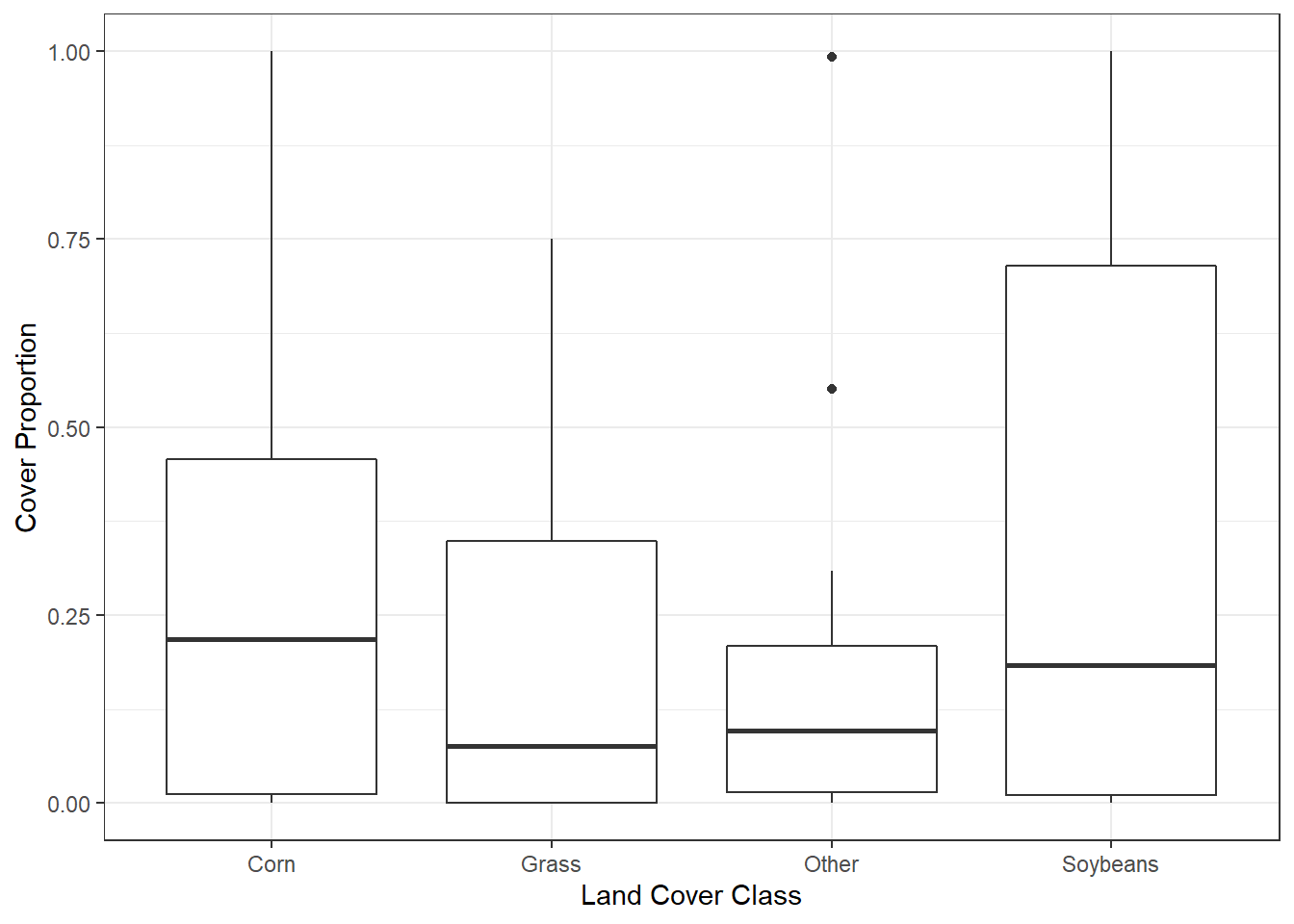
FIGURE 10.12: Percentage of crop types sampled within plot buffers.
10.5 Practice
Repeat the stream buffer analysis for the Hidewood Creek watershed using a 200 m stream buffer width.
Generate 10 random plot locations in the North Deer Creek watershed using a different random number seed (12345). Reclassify the CDL data into three classes: 1) Corn plus soybean, 2) grass, and 3) all other crop types and generate a boxplot of their distributions within 300 m buffers around the plots.