Chapter 11 Application - Wildfire Severity Analysis
This chapter addresses the application of satellite remote sensing data for mapping wildfire severity patterns and analyzing their associations with the wildland-urban interface and topography. Fire severity is defined as the level of impact that a fire has on the ecosystem that was burned. In forest ecosystems, major aspects of severity include the death of overstory trees and combustion of soil organic matter. One way to measure fire severity is to obtain remotely-sensed imagery before and after the fire and assess the differences in the images to measure how much change in vegetation and soils has occurred after the fire (Miller and Thode 2007). These data can be combined with other social and environmental datasets to study the determinants and effects of fire severity. Understanding these relationships is important for developing management strategies to sustain the beneficial ecological effects of fire while reducing the negative impacts on people and property.
In this chapter, wildfire data will be analyzed by applying the techniques covered in early chapters and introducing a new statistical modeling technique to characterize the influences of environmental factors on spatial patterns of fire severity. Most of the R packages needed to conduct these analyses have been introduced in the previous chapters. In addition, the mgcv package (Wood 2022) will be used for generalized additive modeling, and the visreg package (Breheny and Burchett 2020) will be used to help visualized the model results.
library(tidyverse)
library(terra)
library(ggspatial)
library(sf)
library(cowplot)
library(mgcv)
library(visreg)
source("rasterdf.R")
11.1 Remote Sensing Image Analysis
We will use Landsat imagery to develop a map of fire severity for the High Park fire, which burned more than 87,000 acres near Fort Collins, CO in 2012. A series of Landsat satellites have provided high-resolution (30 m) multispectral imagery beginning with the launch of Landsat 4 in 1984. The data for this analysis were obtained from the Monitoring Trends in Burn Severity (MTBS) project (https://www.mtbs.gov/). This project uses satellite remote sensing to produce maps of fire severity for every major fire that occurs in the United States (Eidenshink et al. 2007). For illustration, this chapter will start with the raw satellite imagery provided by MTBS and show how it is processed to develop an index of burn severity. To start, two Landsat images are imported. One was collected in 2011 before the fire, and one was collected in 2013 after the fire.
landsat_pre <- rast("co4058910540420120609_20110912_l5_refl.tif")
landsat_post <- rast("co4058910540420120609_20130901_l8_refl.tif")
Each of the resulting SpatRaster objects is a raster of 30 m square cells with 850 rows by 1149 columns. The landsat_pre object contains Landsat 5 data with six spectral bands.
nrow(landsat_pre)
## [1] 850
ncol(landsat_pre)
## [1] 1149
res(landsat_pre)
## [1] 30 30
nlyr(landsat_pre)
## [1] 6
ext(landsat_pre)[1:4]
##    xmin    xmax    ymin    ymax
## -801045 -766575 1985745 2011245
The landsat_post object contains Landsat 8 data with eight spectral bands. The first six bands of each layer match up, and the seventh and eighth bands in landsat_post contain two additional bands that we will not use here.
nrow(landsat_post)
## [1] 850
ncol(landsat_post)
## [1] 1149
res(landsat_post)
## [1] 30 30
nlyr(landsat_post)
## [1] 8
ext(landsat_post)[1:4]
##    xmin    xmax    ymin    ymax
## -801045 -766575 1985745 2011245
In general, R is not as powerful for visualizing and exploring raw remote sensing imagery as dedicated remote sensing software. However, it is helpful to be able to quickly view remotely sensed images in R. The plotRGB() function in the terra package displays the Landsat images as false color composites, with the short-wave infrared band (layer 6) displayed as red, near-infrared (layer 4) displayed as green, and green (layer 2) displayed as blue. The pre-fire image is dominated by healthy vegetation, which reflects near-infrared radiation and appears green in the false-color image (Figure 11.1).
plotRGB(landsat_pre,
        r = 6,
        g = 4,
        b = 2)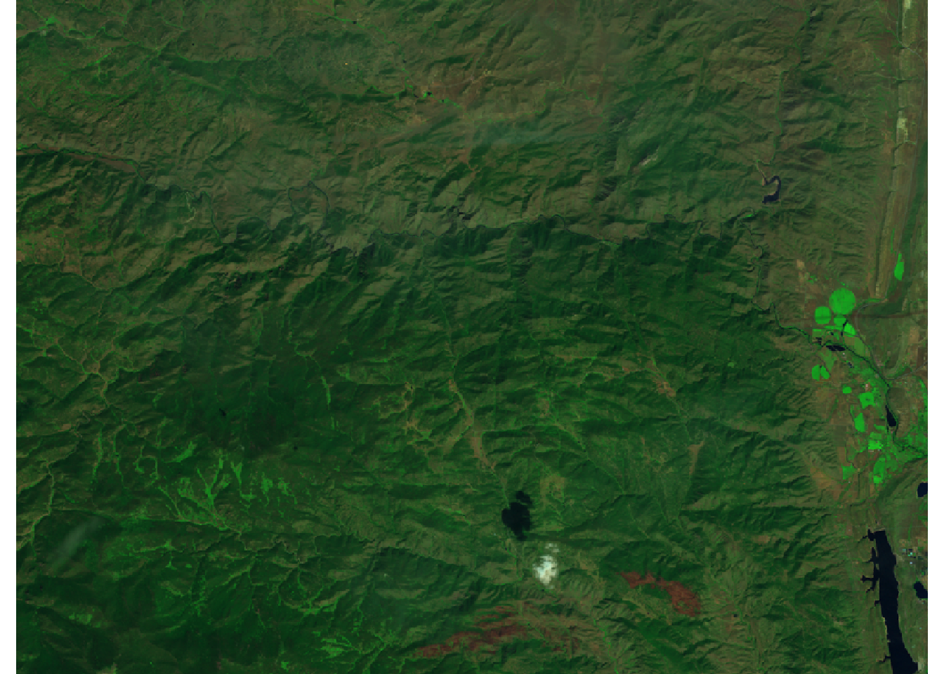
FIGURE 11.1: False-color image of 2011 pre-fire vegetation condition on the High Park fire.
Large areas of trees were killed by the fire in 2012, and soils in the burned areas were blackened by char. These areas reflect less near-infrared radiation and more short-wave infrared radiation. As a result, much of the false color image appears reddish brown in 2013 after the fire (Figure 11.2).
plotRGB(landsat_post,
        r = 6,
        g = 4,
        b = 2)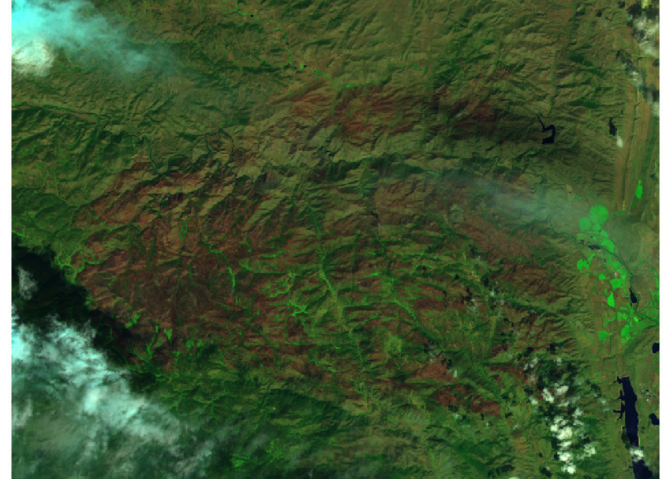
FIGURE 11.2: False-color image of 2013 post-fire vegetation condition on the High Park fire.
Pre- and post-fire landscape conditions are characterized using the normalized burn ratio (NBR) index. This index measures the contrast between the near-infrared band (layer 4), which is highest in areas of healthly green vegetation, and a shortwave-infrared band (layer 6), which is highest in unvegetated areas with blackened or exposed soils. Thus, the NBR is highest in areas with undisturbed forest vegetation and lowest in areas where fire has killed most or all of the vegetation and blackened the soil. The differenced normalized burn index (DNBR) is calculated as the difference between pre- and post-fire NBR, providing an estimate of the effects of the fire on vegetation and soils.
nbr_pre <- 1000 * (landsat_pre[[4]] - landsat_pre[[6]]) /
  (landsat_pre[[4]] + landsat_pre[[6]])
nbr_post <- 1000 * (landsat_post[[4]] - landsat_post[[6]]) /
  (landsat_post[[4]] + landsat_post[[6]])
dnbr <- nbr_pre - nbr_post
The pre-fire and post-fire NBR rasters are combined into a multilayer raster object and mapped (Figure 11.3). A scale bar is also added for reference. Because increasing levels of NBR are generally associated with increasing tree cover, a light-yellow-to-dark-green color ramp is used. There are more areas with low NBR after the fire, but some locations already had low NBR before the fire.
nbr_stack <- c(nbr_pre, nbr_post)
names(nbr_stack) <- c("Pre-fire NBR", "Post-fire NBR")
nbr_stack_df <- rasterdf(nbr_stack)

ggplot(nbr_stack_df) +
  geom_raster(aes(x = x,
                  y = y,
                  fill = value)) +
  scale_fill_gradient(name = "NBR",
                       low = "lightyellow",
                       high = "darkgreen") +
  coord_sf(expand = FALSE) +
  annotation_scale(location = 'bl') +
  facet_wrap(facets = vars(variable),
             ncol = 1) +
  theme_void()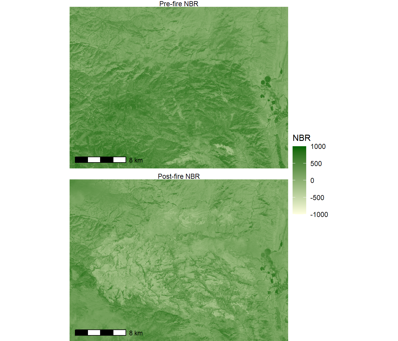
FIGURE 11.3: Pre- and post-fire NBR indices for the High Park fire.
The DNBR index highlights locations where vegetation changed after the fire (Figure 11.4). DNBR is centered at zero, with positive values indicating decreases in NBR and negative values indicating increases. Therefore, the scale_fill_gradient2() is used to create a bicolor ramp centered at zero.
dnbr_df <- rasterdf(dnbr)

ggplot(dnbr_df) +
  geom_raster(aes(x = x,
                  y = y,
                  fill = value)) +
  scale_fill_gradient2(name = "DNBR",
                       low = "blue",
                       high = "red",
                       midpoint = 0) +
  coord_sf(expand = F) +
  annotation_scale(location = 'bl') +
  theme_void()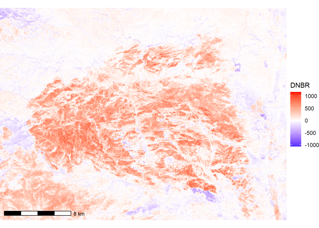
FIGURE 11.4: DNBR index for the High Park fire.
11.2 Burn Severity Classification
The DNBR index will be used to classify the image into discrete levels of burn severity. The classify() function is used to assign severity classes based on DNBR. Previous applications of classify() with land cover data used one-to-one lookup tables to assign each raster value to a new class. Because DNBR is a continuous variable, it is necessary to use a lookup table based on ranges of values.
The easiest way to do this is to create a matrix with three columns: the first column contains the lower value of each range, the second column contains the upper value of each range, and the third column contains the new value to be assigned to the range. The matrix() function takes a vector of data, and the ncol = 3 and byrow = TRUE arguments indicate that the first three values will be the first row, the second three values with be the second row, etc. Then, the classify() function is used with the raster dataset to be reclassified as the first argument and the lookup table as the second argument.
rclas <- matrix(c(-Inf, -970, NA,  # Missing data
                  -970, -100, 5,   # Increased greenness
                  -100, 80, 1,     # Unburned
                  80, 265, 2,      # Low severity
                  265, 490, 3,     # Moderate severity
                  490, Inf, 4),    # High severity
                  ncol = 3, byrow = T)

severity <- classify(dnbr, rclas)
Inferring fire severity from vegetation change is based on the assumption that the observed changes are the result of the wildfire and not other drivers of land cover and land use change. Therefore, it is advisable to mask the fire severity raster to the known perimeter of the wildfire. This can be accomplished by reading in the fire boundary, rasterizing it to match the classified fire severity raster, and masking the areas outside of the fire perimeter.
fire_bndy <- st_read("co4058910540420120609_20110912_20130901_bndy.shp",
                     quiet = TRUE)
bndy_rast <- rasterize(vect(fire_bndy),
                       severity,
                       field = "Event_ID")
severity <- mask(severity, bndy_rast)
Vectors of colors and names for the five severity classes are specified and are used with the masked fire severity dataset to generate a map (Figure 11.5). High severity indicates areas where crown fire or high-intensity surface fire killed most of the trees. Low severity indicates areas with low-intensity surface fires where most trees survived. Mixed severity indicates an intermediate level of tree survival. In some cases, rapid postfire growth can occur where there was sparse vegetation prior to the fire and burning triggers a flush of grasses and other herbaceous vegetation growth.
SCcolors = c("darkgreen",
             "cyan3",
             "yellow",
             "red",
             "green")
SCnames = c("Unburned",
            "Low",
            "Moderate",
            "High",
            "> Green")
severity_df <- rasterdf(severity)

ggplot(severity_df) +
  geom_raster(aes(x = x,
                  y = y,
                  fill = as.character(value))) +
  scale_fill_manual(name = "Severity Class",
                    values = SCcolors,
                    labels = SCnames,
                    na.translate = FALSE) +
  annotation_scale(location = 'bl') +
  coord_fixed(expand = F) +
  theme_void()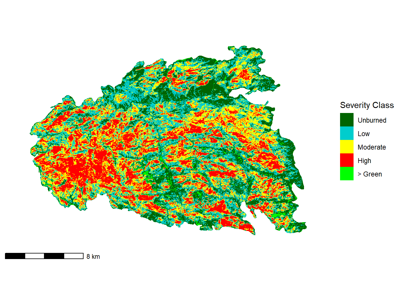
FIGURE 11.5: Severity classes for the High Park fire.
11.3 The Wildland-Urban Interface
We will analyze these burn severity patterns by overlaying them with several other geospatial datasets. The wildland-urban interface (WUI) is defined as the zone where houses and other infrastructure are location in close vicinity to wildland vegetation. The “intermix” is characterized by houses and other buildings scattered throughout wildlands at low densities, whereas the “interface” is the zone where denser urban settlements are adjacent to wildland vegetation (Radeloff et al. 2005). The WUI is a significant concern for fire management because of the difficulty and expense of protecting large numbers of structures, particularly when they are dispersed over large areas of intermix WUI. Thus, there is interest in knowing the degree to which large wildfires like the High Park fire are occurring within or close to the WUI.
The WUI can be identified via geospatial analysis that overlays vegetation data from the NLCD with housing density data from the US Census. WUI data for the United States can be downloaded on a state-by-state basis from http://silvis.forest.wisc.edu/data/wui-change/. Because of the large sizes of these statewide datasets, this example uses a smaller version that has already been clipped to a portion of Colorado.
wui <- st_read("co_wui_cp12_clip.shp", quiet=TRUE)The WUI dataset will need to be rasterized and cropped to match the geometric characteristics of the fire severity dataset. Both datasets are in a similar Albers Equal Area coordinate system, although there is a minor difference in the definition of the spheroid.
writeLines(st_crs(wui)$WktPretty)
## PROJCS["NAD_1983_Albers",
##     GEOGCS["NAD83",
##         DATUM["North_American_Datum_1983",
##             SPHEROID["GRS 1980",6378137,298.257222101],
##             AUTHORITY["EPSG","6269"]],
##         PRIMEM["Greenwich",0],
##         UNIT["Degree",0.0174532925199433]],
##     PROJECTION["Albers_Conic_Equal_Area"],
##     PARAMETER["latitude_of_center",23],
##     PARAMETER["longitude_of_center",-96],
##     PARAMETER["standard_parallel_1",29.5],
##     PARAMETER["standard_parallel_2",45.5],
##     PARAMETER["false_easting",0],
##     PARAMETER["false_northing",0],
##     UNIT["metre",1,
##         AUTHORITY["EPSG","9001"]],
##     AXIS["Easting",EAST],
##     AXIS["Northing",NORTH]]
writeLines(st_crs(severity)$WktPretty)
## PROJCS["USA_Contiguous_Albers_Equal_Area_Conic_USGS_version",
##     GEOGCS["NAD83",
##         DATUM["North_American_Datum_1983",
##             SPHEROID["GRS 1980",6378137,298.257222101004]],
##         PRIMEM["Greenwich",0],
##         UNIT["degree",0.0174532925199433,
##             AUTHORITY["EPSG","9122"]],
##         AUTHORITY["EPSG","4269"]],
##     PROJECTION["Albers_Conic_Equal_Area"],
##     PARAMETER["latitude_of_center",23],
##     PARAMETER["longitude_of_center",-96],
##     PARAMETER["standard_parallel_1",29.5],
##     PARAMETER["standard_parallel_2",45.5],
##     PARAMETER["false_easting",0],
##     PARAMETER["false_northing",0],
##     UNIT["metre",1,
##         AUTHORITY["EPSG","9001"]],
##     AXIS["Easting",EAST],
##     AXIS["Northing",NORTH]]
The WUI vector data are first reprojected to match the coordinate system of the fire severity dataset and are then cropped to its boundary. The map shows the WUI polygons, which correspond to U.S. Census blocks, in the different WUI classes (Figure 11.6).
wui_reproj <- st_transform(wui, crs(severity))
wui_crop <- st_crop(wui_reproj, severity)

ggplot(data = wui_crop) +
  geom_sf(aes(fill = as.character(WUIFLAG10))) +
  scale_fill_manual(name = "WUI Class",
                    values = c("Gray", "Orange", "Red"),
                    labels = c("Non-WUI", "Intermix", "Interface"),
                    na.translate = FALSE) +
  coord_sf(expand = FALSE) +
  theme_void()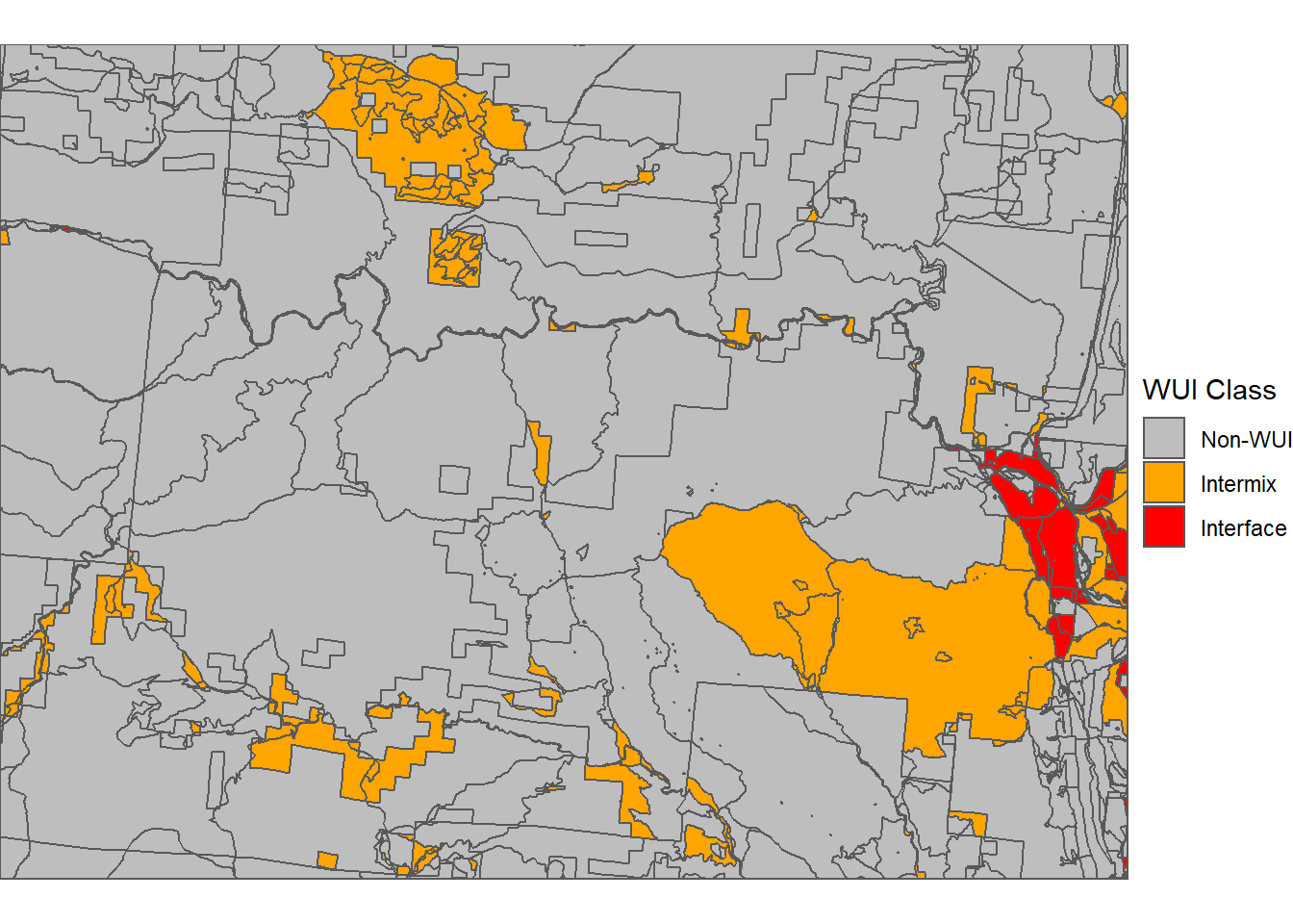
FIGURE 11.6: Vector data characterizing WUI classes for the High Park fire.
Next, the rasterize() function is used to convert the vector WUI dataset into a raster layer with the same geometric characteristics as the fire severity layer. The WUIFLAG10 field provides the values for the output raster: 0 = Non-WUI, 1 = Intermix, and 2 = Interface (Figure 11.7).
wui_rast <- rasterize(vect(wui_crop),
                      severity,
                      field = "WUIFLAG10")
wui_rast_df <- rasterdf(wui_rast)

ggplot(wui_rast_df) +
  geom_raster(aes(x = x,
                  y = y,
                  fill = as.character(value))) +
  scale_fill_manual(name = "WUI Class",
                    values = c("Gray", "Orange", "Red"),
                    labels = c("Non-WUI", "Intermix", "Interface"),
                    na.translate = FALSE) +
  coord_sf(expand = FALSE) +
  theme_void()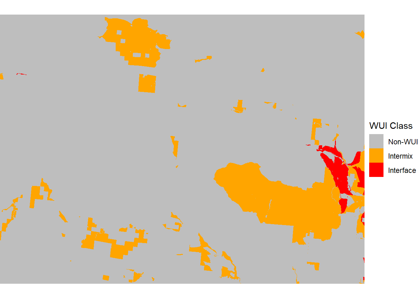
FIGURE 11.7: Raster data characterizing WUI classes for the High Park fire.
Distance from the WUI is calculated using the distance() function. Distance is calculated for all cells with an NA value to the nearest cell that does not have an NA value. Therefore, the WUI raster dataset must first be reclassified into a raster where all WUI cells have a value and all non-WUI cells are NA. This type of simple conditional assignment can be made using the ifel() function, which takes a logical expression as the first argument, the value to assign if the expression is TRUE as the second argument, and the value to assign if the expression if FALSE as the third argument.
wui_na <- ifel(wui_rast == 0, NA, 1)
wui_dist <- distance(wui_na)
The raster containing continuous distance values is then reclassified with the classify() function into a discrete raster with four distance classes using the same approach applied previously for DNBR. The distance to WUI classes is displayed as a categorical map (Figure 11.8).
rclas <- matrix(c(-Inf, 0, 1,
                  0, 1000, 2,
                  1000, 3000, 3,
                  3000, Inf, 4),
                ncol = 3, byrow = T)
wui_rcls <- classify(wui_dist, rcl = rclas)
wui_rcls_df <- rasterdf(wui_rcls)

ggplot(wui_rcls_df) +
  geom_raster(aes(x = x,
                  y = y,
                  fill = as.factor(value))) +
  scale_fill_manual(name = "WUI Distance",
                    values = c("Gray",
                               "Red",
                               "Orange",
                               "Yellow"),
                    labels = c("WUI",
                               "0-1000",
                               "1000-3000",
                               "> 3000"),
                    na.translate = FALSE) +
  coord_sf(expand = FALSE) +
  theme_void()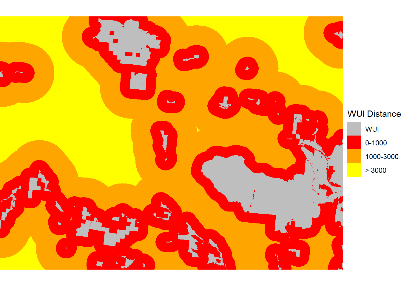
FIGURE 11.8: Raster data distance from the nearest WUI for the High Park fire.
The crosstab() function is used to calculate the distribution of fire severity classes for every WUI distance class. The output is then manipulated to give the columns shorter names, convert counts of 30 m square cells to hectares, and convert the WUI distance and severity variables to labeled factors.
wui_xtab <- crosstab(c(wui_rcls,
                       severity))
wui_df <- as_tibble(wui_xtab)

wui_df <- wui_df %>%
  rename(wuidist = 1, sev = 2, ha = 3) %>%
  mutate(ha = ha * 900 / 10000,
         wuidist = factor(wuidist,
                          levels = 1:4,
                          labels =  c("WUI",
                                      "0-1000",
                                      "1000-3000",
                                      "> 3000")),
         sev = factor(sev,
                      levels = 1:5,
                      labels = SCnames))
A barchart comparing these categories shows that there is an association between distance tot the WUI and fire severity (Figure 11.9). Inside the WUI and close to the WUI, unburned and low severity are the most common severity classes. However, the relative amounts of moderate and high severity classes increase with distance from the WUI, and at the farthest distance, high severity is the most abundant class.
ggplot(data = wui_df) +
  geom_bar(aes(x = wuidist,
               y = ha,
               fill = sev),
           position = "dodge",
           stat = "identity") +
  scale_fill_manual(name = "Severity Class",
                    values = SCcolors) +
  labs(x = "WUI Distance Class",
       y = "Hectares") +
  theme_bw()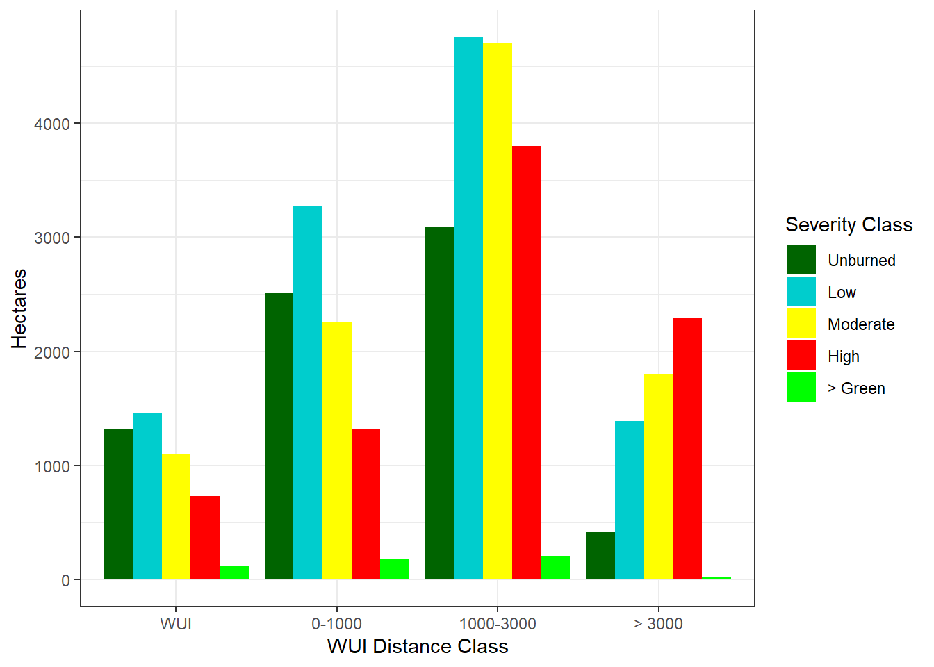
FIGURE 11.9: Raster data distance from the nearest WUI for the High Park fire.
11.4 Topographic Effects
The next analysis will explore the relationship between the observed pattern of fire severity and topography. Elevation is often related to fire severity because the climate is strongly influenced by elevation, and different forest vegetation types and fire regimes are found at different elevations as a result. In the Colorado Front range, higher-elevation forests are often dominated by lodgepole pine (Pinus contorta), which occurs in dense stands that are susceptible to high-severity crown fires. Lower elevations are dominated by other tree species such as Douglas-fir (Pseudotsuga menziesii) and ponderosa pine (Pinus ponderosa) that are more like to survive when an area is burned. Wildfires are also sensitive to slope angle, spreading more rapidly up and more slowly down steep slopes. South-facing slopes receive more direct solar radiation than north-facing slopes. The resulting drier conditions affect the vegetation community and reduce fuel moisture, which can lead to higher fire severity on south-facing slopes.
11.4.1 Data Processing
The elevation data were obtained from the National Elevation Dataset (NED) through the United States Geological Survey’s National Map (https://www.usgs.gov/the-national-map-data-delivery). These data are in a geographic projection and must be reprojected to match the fire severity data. By providing the severity raster as the second argument to the project() function, the output is projected to the same CRS and also matched to the raster geometry (origin, cell size, and extent) of the existing fire severity raster.
elev <- rast("USGS_1_n41w106_20220331.tif")
writeLines(st_crs(elev)$WktPretty)
## GEOGCS["NAD83",
##     DATUM["North_American_Datum_1983",
##         SPHEROID["GRS 1980",6378137,298.257222101004]],
##     PRIMEM["Greenwich",0],
##     UNIT["degree",0.0174532925199433,
##         AUTHORITY["EPSG","9122"]],
##     AXIS["Latitude",NORTH],
##     AXIS["Longitude",EAST],
##     AUTHORITY["EPSG","4269"]]
elev_crop <- project(elev,
                     severity,
                     method = "bilinear")
The map shows that elevation in the Colorado Front Range generally increases from east to west and that there are several drainages and ridgelines within the boundary of the High Park fire (Figure 11.10).
elev_crop_df <- rasterdf(elev_crop)
ggplot(elev_crop_df) +
  geom_raster(aes(x = x, y = y, fill = value)) +
  scale_fill_distiller(name = "Elevation (m)",
                      palette = "Oranges") +
  geom_sf(data = fire_bndy, fill = NA) +
  coord_sf(expand = FALSE) +
  theme_void()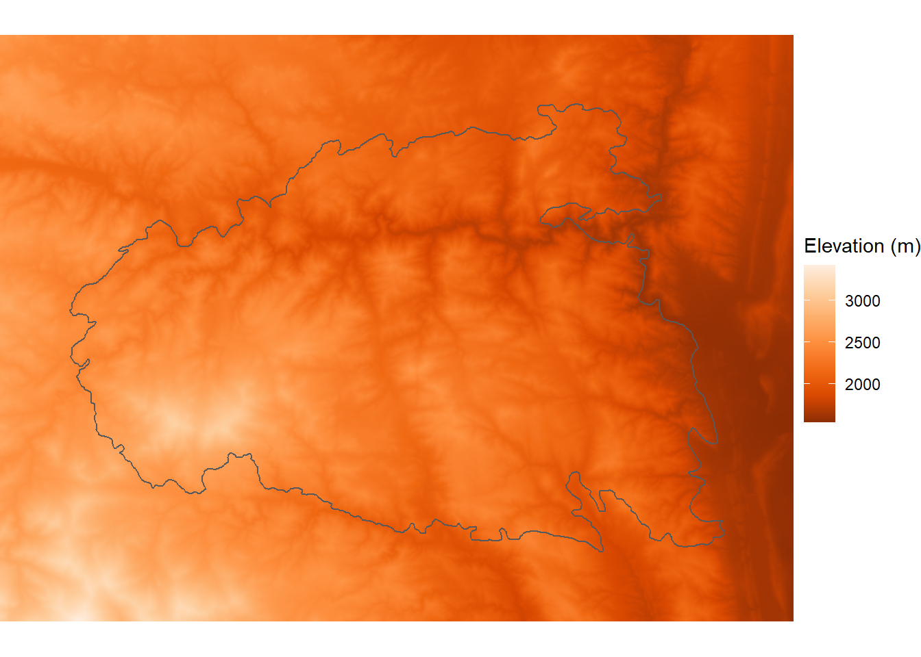
FIGURE 11.10: Elevation within the boundary of the High Park fire.
Slope angle can be calculated using the terrain() function and then mapped (Figure 11.11).
slopedeg <- terrain(elev_crop,
                    v="slope",
                    unit="degrees")
slopedeg_df <- rasterdf(slopedeg)
ggplot(slopedeg_df) +
  geom_raster(aes(x = x, y = y, fill = value)) +
  scale_fill_distiller(name = "Slope (degrees)",
                       palette = "Oranges") +
  geom_sf(data = fire_bndy, fill = NA) +
  coord_sf(expand = FALSE) +
  theme_void()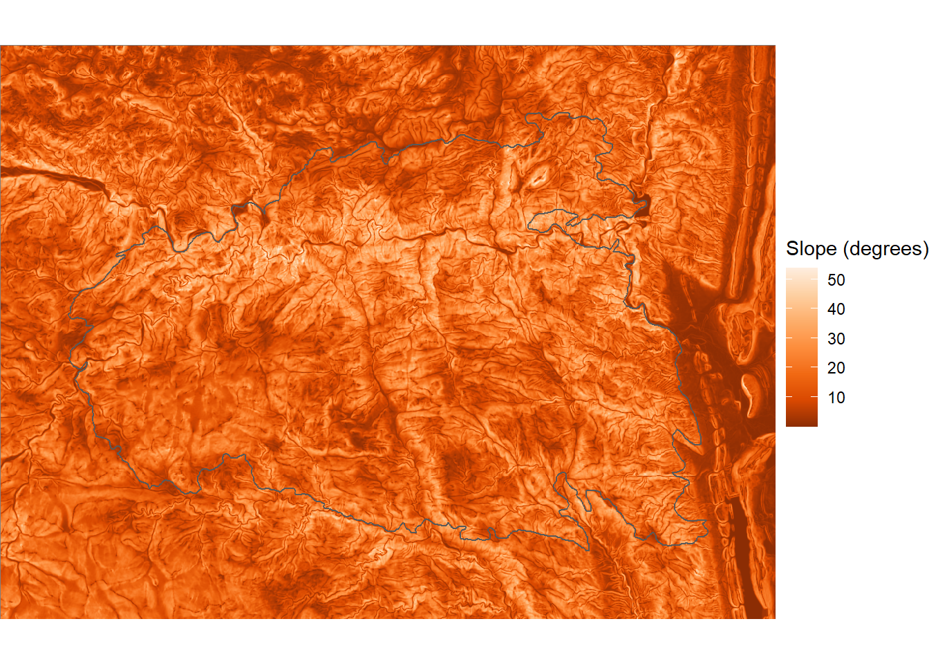
FIGURE 11.11: Slope angle within the boundary of the High Park fire.
Slope aspect is similarly calculated using the terrain() function with units as radians. A north aspect will have a value of 0, an east aspect a value of 0.5\(\pi\), a south aspect a value of \(\pi\), and a west aspect a value of 1.5\(\pi\). The cos() function is then used to convert the circular aspect angle into a linear north-south index, where values of 1 indicate north-facing slopes and values of -1 indicate south-facing slopes (Figure 11.12).
aspect <- terrain(elev_crop, v="aspect", unit="radians")
nsaspect <- cos(aspect)
nsaspect_df <- rasterdf(nsaspect)

ggplot(nsaspect_df) +
  geom_raster(aes(x = x, y = y, fill = value)) +
  scale_fill_distiller(name = "Aspect (N-S index)",
                       palette = "Oranges") +
  geom_sf(data = fire_bndy, fill = NA) +
  coord_sf(expand = FALSE) +
  theme_void()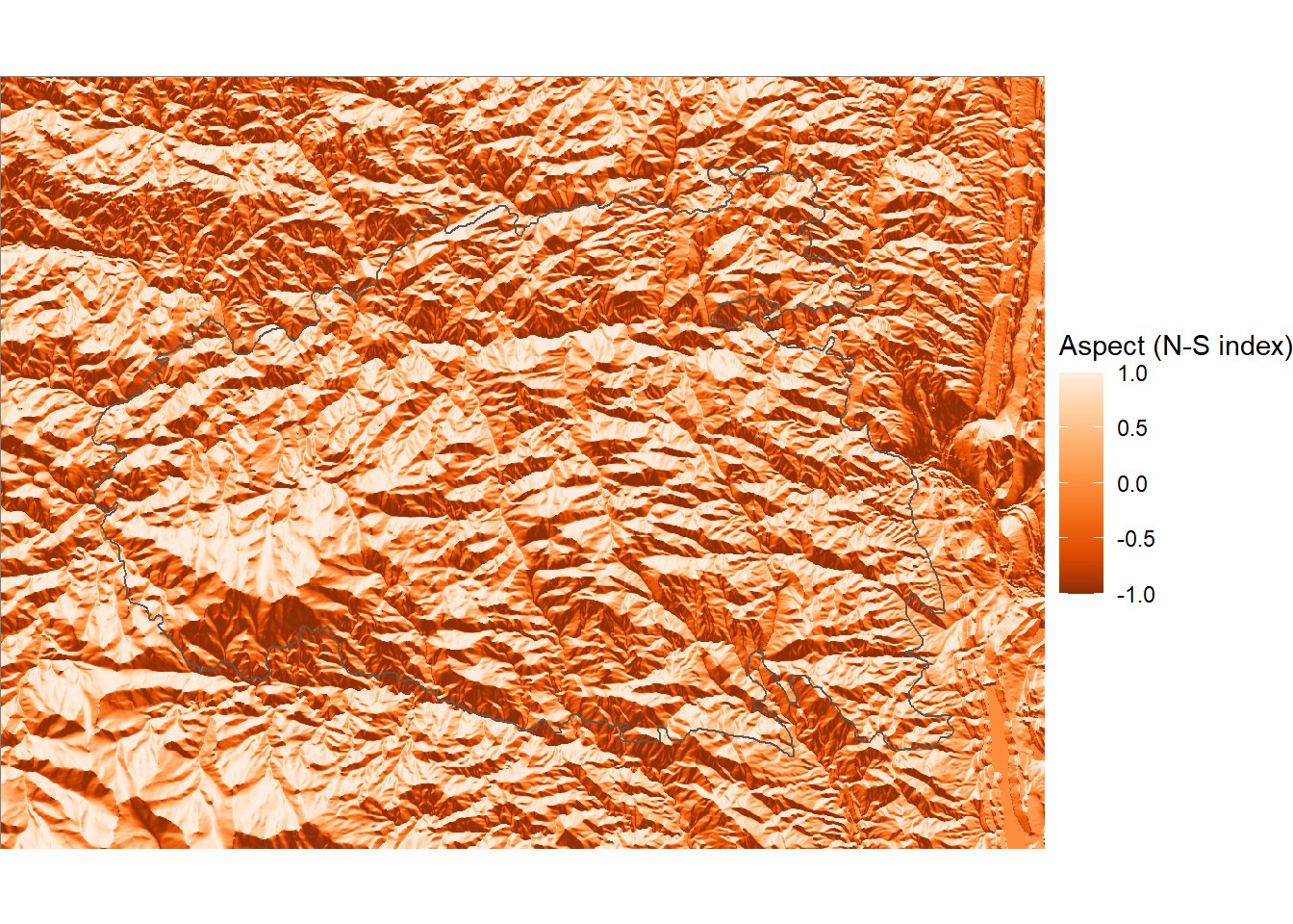
FIGURE 11.12: North-south aspect index within the boundary of the High Park fire.
The sin() function is similarly used to create an east-west index where east-facing slopes have a value of 1 and west-facing slopes have a value of -1 (Figure 11.13).
ewaspect <- sin(aspect)
ewaspect_df <- rasterdf(ewaspect)

ggplot(ewaspect_df) +
  geom_raster(aes(x = x, y = y, fill = value)) +
  scale_fill_distiller(name = "Aspect (E-W index)",
                       palette = "Oranges") +
  geom_sf(data = fire_bndy, fill = NA) +
  coord_sf(expand = FALSE) +
  theme_void()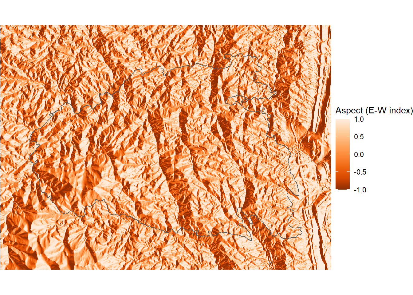
FIGURE 11.13: East-west aspect index within the boundary of the High Park fire.
To analyze the relationships between fire severity and these topographic indices, a sample of points inside the boundary of the High Park fire is needed. The first step is to combine DNBR with the topographic indices into a multilayer raster object.
fire_stack <- c(dnbr,
                elev_crop,
                slopedeg,
                nsaspect,
                ewaspect)
The st_sample() function is used to generate a set of random points as was done in Chapter 10. In this case, several additional arguments are provided. The points are constrained to fall inside the fire_bndy polygon data set. The type = SSI argument indicates that a simple sequential inhibition process will be used to generate the points. After the first random point is generated, subsequent points are only accepted if they are farther than a threshold distance from the nearest point. The r argument indicates the minimum distance between points, and n indicates the number of points to sample. The resulting sample_pts dataset is in the same coordinate reference system as fire_bndy, but the coordinate reference system is not automatically defined and must be specified manually.
set.seed(23456)
sample_pts <- st_sample(
  fire_bndy,
  type = "SSI",
  r = 500,
  n = 300
)
st_crs(sample_pts)
## Coordinate Reference System: NA
st_crs(sample_pts) <- st_crs(fire_bndy)
11.4.2 Generalized Additive Modeling
Setting a minimum distance is desireable in this case because the values of nearby raster cells tend to be strongly correlated with one another, and using widely-spaced points help to ensure broad coverage and maximize the independence of each sample (Figure 11.14). As discussed in Chapter 10, setting a random number seed ensures that running the code multiple times will generate the same sequence of random numbers.
ggplot(dnbr_df) +
  geom_raster(aes(x = x,
                  y = y,
                  fill = value)) +
  scale_fill_gradient2(name = "DNBR",
                       low = "blue",
                       high = "red",
                       midpoint = 0) +
  geom_sf(data = fire_bndy, fill = NA) +
  geom_sf(data = sample_pts) +
  coord_sf(expand = F) +
  theme_void()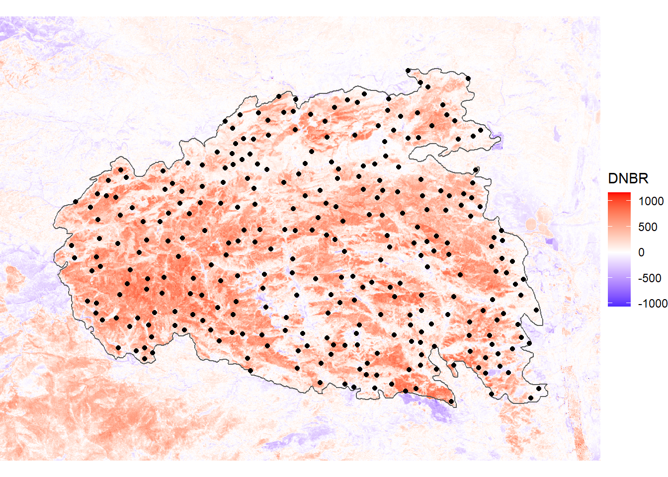
FIGURE 11.14: Sample points and fire boundary overlaid on the DNBR index for the High Park fire.
The extract() function is then used to extract raster data at these point locations, and the columns of the resulting data frame are renamed.
fire_pts <- extract(fire_stack, vect(sample_pts))

fire_pts <- rename(fire_pts,
                   dnbr = 2,
                   elevation = 3,
                   slope = 4,
                   nsaspect = 5,
                   ewaspect = 6)
To explore the relationships between fire severity and topography, a generalized additive model (GAM) is applied using the gam() function from the mgcv library. The specification of the model is similar to the linear models that were previously run using the lm() function. A model formula is specified with dependent variables on the left side of the tilde (~) and independent variables separated by the plus (+) symbol on the right side. In addition, each of the independent variables is wrapped in the s() function, which by default models the dependent variable as a smooth thin-plate spline function. This approach is warranted when the underlying relationships are not assumed to be linear.
fire_gam <- gam(dnbr ~
                  s(elevation) +
                  s(slope) +
                  s(nsaspect) +
                  s(ewaspect),
                data = fire_pts)
The summary method for a gam object looks generally similar to that of an lm() object, but upon close inspection, has some important differences. For example, there is a table of test statistics and p-values for each of the independent variables, but there are no coefficient values as with a linear model. The estimated degrees of freedom (edf) provides information about the degree of non-linearity in the relationships, with higher values indicating more complex non-linear relationships.
class(fire_gam)
## [1] "gam" "glm" "lm"
summary(fire_gam)
##
## Family: gaussian
## Link function: identity
##
## Formula:
## dnbr ~ s(elevation) + s(slope) + s(nsaspect) + s(ewaspect)
##
## Parametric coefficients:
##             Estimate Std. Error t value Pr(>|t|)
## (Intercept)   272.54      10.23   26.63   <2e-16 ***
## ---
## Signif. codes:
## 0 '***' 0.001 '**' 0.01 '*' 0.05 '.' 0.1 ' ' 1
##
## Approximate significance of smooth terms:
##                edf Ref.df      F  p-value
## s(elevation) 5.489  6.656 17.609  < 2e-16 ***
## s(slope)     2.708  3.418  9.257 4.21e-06 ***
## s(nsaspect)  1.000  1.000 53.578  < 2e-16 ***
## s(ewaspect)  4.351  5.323  1.547    0.167
## ---
## Signif. codes:
## 0 '***' 0.001 '**' 0.01 '*' 0.05 '.' 0.1 ' ' 1
##
## R-sq.(adj) =  0.411   Deviance explained = 43.8%
## GCV =  33017  Scale est. = 31416     n = 300
To understand the smoothed relationships modeled by a GAM, they need to be plotted. The gam object has a plot() methods that uses base R graphics to graph the partial residuals as a function of each independent variables. These partial residuals represent the relationships between DNBR and each topographic index after the removing the modeled effects of all the other topographic indices (Figure 11.15). The output shows that DNBR has a unimodal relationship with elevation that peaks at approximately 2700 meters. The relationship with slope is also unomodal with a peak around 22 degrees. The relationship with the north-south index is linear, with fire severity highest on south-facing aspects. The relationship with the east-west aspect is comparatively weak and does not show a clear pattern.
plot(fire_gam, pages = 1)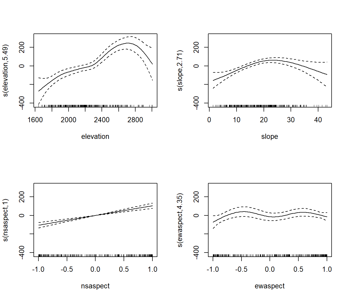
FIGURE 11.15: Partial regression plots for the relationships between topographic indices and fire severity.
Partial regression plots can also be generated using the visreg() function from the visreg package. By specifying the gg = TRUE argument, the plots are generated using ggplot(), and additional ggplot functions can be specified to modify their appearance. Here, a partial plot for each independent variable is generated and saved to a ggplot object.
elev_gg <- visreg(fire_gam,
                  "elevation",
                  gg = TRUE) +
  theme_bw()
slope_gg <- visreg(fire_gam,
                  "slope",
                  gg = TRUE) +
  theme_bw()
nsasp_gg <- visreg(fire_gam,
                   "nsaspect",
                   gg = TRUE) +
  theme_bw()
ewasp_gg <- visreg(fire_gam,
                   "ewaspect",
                   gg = TRUE) +
  theme_bw()
Then, as was shown in Chapter 5, the plot_grid() function from the cowplot package can be used to arrange these multiple plots into a larger multipanel graphic (Figure 11.16).
plot_grid(elev_gg, slope_gg, nsasp_gg, ewasp_gg,
          labels = c("A)", "B)", "C)", "D)",
                     label_size = 12),
          ncol = 2,
          hjust = 0,
          label_x = 0,
          align = "hv")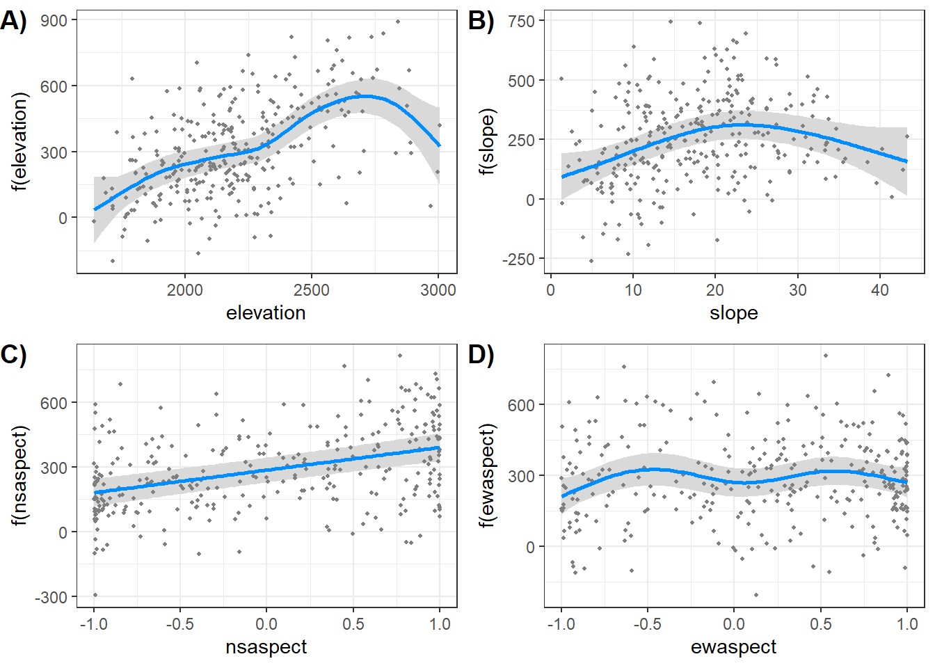
FIGURE 11.16: Partial regression plots for the relationships between topographic indices and fire severity generated using the virdis package.
11.5 Practice
One of the reasons why fire severity was lowest near the WUI may have been that the WUI was concentrated at lower elevations where the forest vegetation is often resilient to fire. Compare these two variables by classifying elevation into four categories and generating a plot like (Figure 11.9) that compares elevation with distance from the WUI.
Another metric of burn severity is the relative differenced normalized burn ratio (RDNBR), which normalizes the DNBR by dividing it by the pre-fire NBR. The RDNBR is calculated as
rdnbr = dnbr/sqrt(abs(nbr_pre)). Calculate the RDNBR for the High Park fire and generate a composite figure that includes both DNBR and RDNBR mapped as continuous variables. Compare the maps and assess the similarities and differences between the two indices.Select and download burn severity data for another wildfire from the MTBS website (https://www.mtbs.gov/) along with elevation data for the same area from the National Map (https://www.usgs.gov/the-national-map-data-delivery). Repeat the analysis of topographic effects on burn severity described in this chapter and see if you obtain similar results in a different location.