1.2 Types of simulations
Before starting the construction of a simulation model, we need to decide upon the principal characteristics of that model. There are various choices to be made, which depend upon the system we are trying to understand.
1.2.1 Stochastic vs deterministic simulations
A model is deterministic if its behavior is entirely predictable. Given a set of inputs, the model will result in a unique set of outputs. A model is stochastic if it has random variables as inputs, and consequently also its outputs are random.
Consider the donut shop example. In a deterministic model we would for instance assume that a new customer arrives every 5 minutes and an employee takes 2 minutes to serve a customer. In a stochastic model we would on the other hand assume that the arrival times and the serving time follows some random variables: for instance, normal distributions with some mean and variance parameters.
In this course we will only consider stochastic simulation, but for illustration we consider now an example of a deterministic simulation.
A social media influencer decides to open a new page and her target is to reach 10k followers in 10 weeks. Given her past experience, she assumes that each week she will get 1.5k new followers that had never followed the page and of her current followers she believes 10% will stop following the page each week. However, 20% of those that the left the page in the past will join again each week. Will she reach her target?
To answer this question we can construct a deterministic simulation. Let \(F_t\) the number of followers at week \(t\) and \(U_t\) the number of users that are unfollowing the profile at week \(t\). Then \[ F_t = F_{t-1} + 1500 - L_{t} + R_{t}, \hspace{1cm} U_t= U_{t-1} + L_{t} - R_{t} \] where \(L_{t}=0.1\cdot F_{t-1}\) is the number of unfollowers from time \(t-1\) to time \(t\), and \(R_{t}=0.2\cdot U_{t-1}\) is the number of users that follow the page back from time \(t-1\) to time \(t\).
To compute the number of followers after ten weeks we can use the R code below. It does not matter if you do not understand it now, we will review R coding in the next chapters.
Ft <- Ut <- Lt <- Rt <- rep(0,11)
for (i in 2:11){
  Lt[i] <- 0.1*Ft[i-1]
  Rt[i] <- 0.2*Ut[i-1]
  Ut[i] <- Ut[i-1] + Lt[i] - Rt[i]
  Ft[i] <- Ft[i-1] + 1500 - Lt[i] + Rt[i]
}
result <- data.frame("Followers" = Ft, "Total Unfollowers" = Ut,
           "Weekly Unfollowers" = Ut, "Weekly Returns" = Rt)
The dataframe result is reported in Table 1.1, showing that she will be able to hit her target of 10k followers since she will have 11619 followers. If we run again the simulation we will obtain the exact same results: there is no stochasticity/uncertainty about the outcome.
| Followers | Total.Unfollowers | Weekly.Unfollowers | Weekly.Returns |
|---|---|---|---|
| 0.000 | 0.000 | 0.000 | 0.0000 |
| 1500.000 | 0.000 | 0.000 | 0.0000 |
| 2850.000 | 150.000 | 150.000 | 0.0000 |
| 4095.000 | 405.000 | 405.000 | 30.0000 |
| 5266.500 | 733.500 | 733.500 | 81.0000 |
| 6386.550 | 1113.450 | 1113.450 | 146.7000 |
| 7470.585 | 1529.415 | 1529.415 | 222.6900 |
| 8529.409 | 1970.591 | 1970.591 | 305.8830 |
| 9570.587 | 2429.413 | 2429.413 | 394.1181 |
| 10599.411 | 2900.589 | 2900.589 | 485.8827 |
| 11619.587 | 3380.413 | 3380.413 | 580.1179 |
The above application could be transformed into a stochastic simulation by allowing the rate at which she gets new followers, unfollowers etc. to be random variables of which we do not know the exact value.
1.2.2 Static vs dynamic simulations
Simulation models that represent the system at a particular point in time only are called static. This type of simulations are often called as Monte Carlo simulations and will be the focus of later chapters.
Dynamic simulation models represent systems as they evolve over time. The simulation of the donut shop during its working hours is an example of a dynamic model.
1.2.3 Discrete vs continuous simulations
Dynamic simulations can be further categorized into discrete or continuous.
Discrete simulation models are such that the variables of interest change only at a discrete set of points in time. The number of people queuing in the donut shop is an example of a discrete simulation. The number of customers changes only when a new customer arrives or when a customer has been served. Figure 1.1 gives an illustration of the discrete nature of the number of customers queuing in the donut shop.
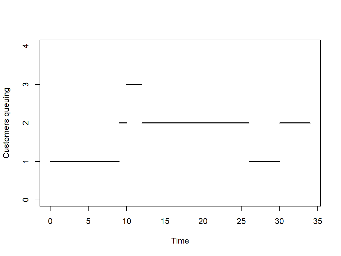
Figure 1.1: Example of a discrete dynamic simulation
Figure 1.1 further illustrates that for specific period of times the system does not change state, that is the number of customers queuing remains constant. It is therefore useless to inspect the system during those times where nothing changes. This prompts the way in which time is usually handled in dynamic discrete simulations, using the so-called next-event technique. The model is only examined and updated when the system is due to change. These changes are usually called events. Looking at Figure 1.1 at time zero there is an event: a customer arrives; at time nine another customer arrives; at time ten another customer arrives; at time twelve a customer is served; and so on. All these are examples of events.
Continuous simulation models are such that the variables of interest change continuously over time. Suppose for instance a simulation model for a car journey was created where the interest is on the speed of the car throughout the journey. Then this would be a continuous simulation model. Figure 1.2 gives an illustration of this.
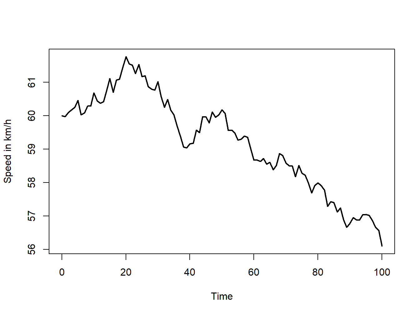
Figure 1.2: Example of a discrete dynamic simulation
In later chapters we will focus on discrete simulations, which are usually called discrete-event simulation. Continuous simulations will not be discussed in these notes.